Dispersion and dissipation error in high-order Runge-Kutta ...
Dispersion and dissipation error in high-order Runge-Kutta ...
Dispersion and dissipation error in high-order Runge-Kutta ...

Create successful ePaper yourself
Turn your PDF publications into a flip-book with our unique Google optimized e-Paper software.
<strong>Dispersion</strong> <strong>and</strong> <strong>dissipation</strong> <strong>error</strong> <strong>in</strong> <strong>high</strong>-<strong>order</strong><br />
<strong>Runge</strong>-<strong>Kutta</strong> discont<strong>in</strong>uous Galerk<strong>in</strong> discretisations of<br />
the Maxwell equations ∗<br />
D. Sármány †‡ M. A. Botchev ‡ J. J. W. van der Vegt ‡<br />
July, 2007<br />
Abstract<br />
Different time-stepp<strong>in</strong>g methods for a nodal <strong>high</strong>-<strong>order</strong> discont<strong>in</strong>uous Galerk<strong>in</strong><br />
discretisation of the Maxwell equations are discussed. A comparison between the<br />
most popular choices of <strong>Runge</strong>-<strong>Kutta</strong> (RK) methods is made from the po<strong>in</strong>t of view<br />
of accuracy <strong>and</strong> computational work. By choos<strong>in</strong>g the strong-stability-preserv<strong>in</strong>g<br />
<strong>Runge</strong>-<strong>Kutta</strong> (SSP-RK) time-<strong>in</strong>tegration method of <strong>order</strong> consistent with the<br />
polynomial <strong>order</strong> of the spatial discretisation, better accuracy can be atta<strong>in</strong>ed<br />
compared with fixed-<strong>order</strong> schemes. Moreover, this comes without a significant<br />
<strong>in</strong>crease <strong>in</strong> the computational work. A numerical Fourier analysis is performed for<br />
this <strong>Runge</strong>-<strong>Kutta</strong> discont<strong>in</strong>uous Galerk<strong>in</strong> (RKDG) discretisation to ga<strong>in</strong> <strong>in</strong>sight<br />
<strong>in</strong>to the dispersion <strong>and</strong> <strong>dissipation</strong> properties of the fully discrete scheme. The<br />
analysis is carried out on both the one-dimensional <strong>and</strong> the two-dimensional fully<br />
discrete schemes <strong>and</strong>, <strong>in</strong> the latter case, on uniform as well as on non-uniform<br />
meshes. It also provides practical <strong>in</strong>formation on the convergence of the <strong>dissipation</strong><br />
<strong>and</strong> dispersion <strong>error</strong> up to polynomial <strong>order</strong> 10 for the one-dimensional fully<br />
discrete scheme.<br />
KEY WORDS: <strong>high</strong>-<strong>order</strong> nodal discont<strong>in</strong>uous Galerk<strong>in</strong> methods; Maxwell<br />
equations; numerical dispersion <strong>and</strong> <strong>dissipation</strong>; strong-stability-preserv<strong>in</strong>g<br />
<strong>Runge</strong>-<strong>Kutta</strong> methods.<br />
1 Introduction<br />
As po<strong>in</strong>ted out <strong>in</strong> an extensive review on the state of the art of computational electromagnetics<br />
[16], <strong>in</strong> many cases f<strong>in</strong>ite-difference time-doma<strong>in</strong> (FDTD) schemes [33, 37]<br />
are undoubtedly the most popular methods among physicists <strong>and</strong> eng<strong>in</strong>eers to solve the<br />
∗ This research was supported by the Dutch government through the national program BSIK: knowledge<br />
<strong>and</strong> research capacity, <strong>in</strong> the ICT project BRICKS (http://www.bsik-bricks.nl), theme MSV1.<br />
† Correspond<strong>in</strong>g author, d.sarmany@math.utwente.nl.<br />
‡ Department of Applied Mathematics, University of Twente, P.O. Box 217, 7500 AE Enschede, Netherl<strong>and</strong>s.<br />
E-mail: [d.sarmany,m.a.botchev,j.j.w.v<strong>and</strong>ervegt]@math.utwente.nl.<br />
1
time-doma<strong>in</strong> Maxwell equations numerically. This popularity is ma<strong>in</strong>ly due to their simplicity<br />
<strong>and</strong> efficiency <strong>in</strong> discretis<strong>in</strong>g simple-doma<strong>in</strong> problems. However, their <strong>in</strong>ability to<br />
effectively h<strong>and</strong>le complex geometries prompted some scientists to search for alternatives<br />
long ago. F<strong>in</strong>ite-element (FE) methods are an obvious alternative, but early efforts were<br />
marred by the fact that st<strong>and</strong>ard cont<strong>in</strong>uous Galerk<strong>in</strong> f<strong>in</strong>ite-element schemes give rise to<br />
non-physical solutions. Most apparent of these are the spurious modes <strong>in</strong> the numerical<br />
solution of the frequency-doma<strong>in</strong> Maxwell equations (see [24] <strong>and</strong> references there<strong>in</strong>).<br />
The revolutionary solution to this problem was to realise that by us<strong>in</strong>g a particular set<br />
of vector basis functions (vector elements such as Nédélec or Whitney elements [20, 29]),<br />
it is possible to mimic many of the special properties of the Maxwell equations at the<br />
discrete level. See [3] <strong>and</strong> [4]. Ever s<strong>in</strong>ce, vector elements have been a viable alternative<br />
to FDTD <strong>and</strong> st<strong>and</strong>ard FE methods <strong>in</strong> computational electrodynamics, especially<br />
for frequency-doma<strong>in</strong> problems with complex geometries. The practical considerations of<br />
both st<strong>and</strong>ard <strong>and</strong> vector f<strong>in</strong>ite elements <strong>in</strong> computational electromagnetics are covered<br />
<strong>in</strong> [24]. For the more theoretical aspects of Nédélec elements we refer to [27].<br />
The need to model electromagnetic wave propagation <strong>in</strong> large <strong>and</strong> complex doma<strong>in</strong>s<br />
<strong>and</strong> over a relatively long time span has <strong>in</strong>creased the dem<strong>and</strong> for <strong>high</strong>-<strong>order</strong> methods.<br />
However, neither <strong>high</strong>-<strong>order</strong> FDTD methods nor <strong>high</strong>-<strong>order</strong> vector FE methods are devoid<br />
of practical drawbacks. High-<strong>order</strong> FDTD methods fail to effectively h<strong>and</strong>le complex<br />
geometries whereas <strong>high</strong>-<strong>order</strong> vector FE methods (based on <strong>high</strong>-<strong>order</strong> Nédélec elements<br />
[29] for example) lead to global mass matrices with relatively large b<strong>and</strong>widths (after<br />
optimal re<strong>order</strong><strong>in</strong>g). The time-<strong>in</strong>tegration schemes to solve such systems are <strong>in</strong> turn<br />
computationally rather expensive. These difficulties have motivated the development<br />
of discont<strong>in</strong>uous Galerk<strong>in</strong> (DG) f<strong>in</strong>ite-element methods [9, 11], together with spectral<br />
element methods [25]. In both the frequency-doma<strong>in</strong> formulation [19, 21, 30, 31, 35]<br />
<strong>and</strong> the time-doma<strong>in</strong> formulation [6, 10, 18, 28] significant progress has been made. One<br />
of the most promis<strong>in</strong>g methods for complicated geometries is the <strong>high</strong>-<strong>order</strong> nodal DG<br />
method of Hesthaven <strong>and</strong> Warburton [18], which proved both accurate <strong>and</strong> efficient for the<br />
spatial discretisation. In time <strong>in</strong>tegration, however, the low-storage <strong>Runge</strong>-<strong>Kutta</strong> (RK)<br />
method the authors applied poses a comparatively str<strong>in</strong>gent time-step constra<strong>in</strong>t, which<br />
may turn out to be the bottleneck for long-time <strong>in</strong>tegration. Furthermore, fixed-<strong>order</strong><br />
time-<strong>in</strong>tegration schemes may spoil the <strong>high</strong>-<strong>order</strong> convergence of the global scheme. In<br />
the meantime, for discont<strong>in</strong>uous formulations of convection-dom<strong>in</strong>ated problems [11] it<br />
has been shown <strong>in</strong> [14] <strong>and</strong> <strong>in</strong> [6] that the time-step restriction may be loosened if we use<br />
Strong-Stability-Preserv<strong>in</strong>g <strong>Runge</strong>-<strong>Kutta</strong> (SSP-RK) methods of one <strong>order</strong> <strong>high</strong>er than the<br />
polynomial <strong>order</strong> of the spatial discretisation.<br />
In this work, we study the behaviour of the <strong>high</strong>-<strong>order</strong> nodal scheme when several of<br />
the best-suited time-<strong>in</strong>tegration methods are used. In particular, we have a closer look<br />
at the dispersion <strong>and</strong> <strong>dissipation</strong> properties of the <strong>Runge</strong>-<strong>Kutta</strong> discont<strong>in</strong>uous Galerk<strong>in</strong><br />
(RKDG) method compris<strong>in</strong>g the nodal <strong>high</strong>-<strong>order</strong> DG method <strong>and</strong> the SSP-RK method.<br />
The ma<strong>in</strong> motivation for us<strong>in</strong>g this particular time-<strong>in</strong>tegration scheme is its relatively<br />
weak time-step restriction. This property implies that we can reta<strong>in</strong> <strong>high</strong>-<strong>order</strong> accuracy<br />
without los<strong>in</strong>g much on the computational work measured as the number of operations.<br />
The literature on the dispersion <strong>and</strong> <strong>dissipation</strong> properties of the DG method has <strong>in</strong><br />
recent years become abundant. A thorough analysis of the dispersion <strong>and</strong> <strong>dissipation</strong><br />
2
ehaviour of the DG method for the transport equation (scalar l<strong>in</strong>ear conservation law)<br />
was given <strong>in</strong> [1], which also provided a proof for earlier conjectures, especially from [22].<br />
The semi-discrete system for the wave equation has also been extensively studied [2, 23,<br />
32]. In particular, the authors <strong>in</strong> [2] provided two different dispersion analyses for the<br />
semi-discrete wave equation on tensor product elements. One for the <strong>in</strong>terior penalty<br />
DG method (IP-DG) of the second-<strong>order</strong> wave equation <strong>and</strong> another for the general DG<br />
method for a first <strong>order</strong> system.<br />
The novelty of this work with regards to the dispersion <strong>and</strong> <strong>dissipation</strong> behaviour<br />
of DG methods lies <strong>in</strong> <strong>in</strong>clud<strong>in</strong>g the time <strong>in</strong>tegration <strong>in</strong> the analysis. We consider the<br />
discretisation of the first-<strong>order</strong> system related to the Maxwell equations, so our scheme<br />
falls <strong>in</strong> the category of what the authors call the ‘general DG method’ <strong>in</strong> [2]. Throughout<br />
this article we apply a fully upw<strong>in</strong>d<strong>in</strong>g numerical flux, s<strong>in</strong>ce it has proved superior–due<br />
to stabilisation <strong>and</strong> lack of spurious modes–to the centered or mixed fluxes for timedependent<br />
problems [19]. In wave-propagation problems it is often more advantageous to<br />
know the convergence rate of the dispersion <strong>and</strong> <strong>dissipation</strong> <strong>error</strong>s than that of the <strong>error</strong><br />
<strong>in</strong> the L 2 -norm. These convergence rates have been established <strong>in</strong> [1] for the semi-discrete<br />
transport equation. For the general DG scheme, to which the nodal DG method discussed<br />
here belongs, it has been shown <strong>in</strong> [2] that us<strong>in</strong>g first-<strong>order</strong> polynomials <strong>in</strong> the spatial<br />
discretisation results <strong>in</strong> a dispersion <strong>error</strong> of <strong>order</strong> O(h 4 ) <strong>and</strong> a <strong>dissipation</strong> <strong>error</strong> of <strong>order</strong><br />
O(h 3 ) for the semi-discrete system. In this work we show, through numerical examples,<br />
how the dispersion <strong>and</strong> <strong>dissipation</strong> <strong>error</strong>s converge <strong>in</strong> the fully discrete <strong>high</strong>-<strong>order</strong> RKDG<br />
scheme for the l<strong>in</strong>ear autonomous form of the Maxwell equations.<br />
The rema<strong>in</strong><strong>in</strong>g part of this article is outl<strong>in</strong>ed as follows. In Section 2 we recall the<br />
system of time-doma<strong>in</strong> Maxwell equations <strong>and</strong> reduce it to the l<strong>in</strong>ear autonomous form.<br />
The spatial discretisation is briefly reviewed <strong>in</strong> Section 3 <strong>and</strong> the RK schemes for the<br />
temporal discretisation <strong>in</strong> Section 4. One-dimensional <strong>and</strong> two-dimensional Fourier analysis<br />
is carried out <strong>in</strong> Section 5, <strong>and</strong> the associated numerical results, along with some<br />
other numerical tests, are presented <strong>in</strong> Section 6. Here we exam<strong>in</strong>e the behaviour of the<br />
dispersion <strong>and</strong> <strong>dissipation</strong> <strong>error</strong>s <strong>in</strong> terms of the mesh size per wave length <strong>and</strong> the size<br />
of the time step. F<strong>in</strong>ally, we sum up our conclusions <strong>in</strong> Section 7.<br />
2 Maxwell equations<br />
We beg<strong>in</strong> with deriv<strong>in</strong>g the dimensionless time-doma<strong>in</strong> form of the Maxwell equations<br />
<strong>in</strong> the three-dimensional doma<strong>in</strong> Ω ⊂ R 3 . Boldface symbols here refer to vector fields,<br />
i.e. fields <strong>in</strong> R 3 → R 3 . With these notations the Maxwell equations read<br />
∂D<br />
∂t = ∇ × H − J,<br />
∂B<br />
∂t<br />
= −∇ × E, (1)<br />
∇ · D = ̺, ∇ · B = 0, (2)<br />
with ( charge distribution ) ̺(x, t), position vector x = (x, y, z) ∈ Ω, the nabla operator<br />
∂<br />
∇ = , ∂ , ∂ <strong>and</strong> time t. The vector valued quantities are the electric field E(x, t),<br />
∂x ∂y ∂z<br />
the electric flux density D(x, t), the magnetic field H(x, t), the magnetic flux density<br />
B(x, t) <strong>and</strong> the electric current J(x, t). For many applications it is reasonable to assume<br />
3
that the materials are isotropic, l<strong>in</strong>ear <strong>and</strong> time-<strong>in</strong>variant. Thus the system of equations<br />
is closed with the l<strong>in</strong>ear constitutive relations<br />
D = ε r E, B = µ r H, (3)<br />
where the scalar quantities ε r (x) <strong>and</strong> µ r (x) are the permittivity <strong>and</strong> permeability, respectively.<br />
Furthermore, Ohm’s law<br />
J = σE<br />
also holds with electric conductivity σ(x, t).<br />
To obta<strong>in</strong> the non-dimensional form of the Maxwell equations (1)–(2), we first <strong>in</strong>troduce<br />
tilded variables to represent the dimensional fields. The special notations ˜ε 0 <strong>and</strong><br />
˜µ 0 st<strong>and</strong> for the dimensional permittivity <strong>and</strong> permeability of vacuum. By us<strong>in</strong>g the<br />
normalised space <strong>and</strong> time variables<br />
x = ˜x˜L,<br />
t = ˜t<br />
˜L/˜c 0<br />
,<br />
with reference length ˜L <strong>and</strong> dimensional speed of light <strong>in</strong> vacuum ˜c 0 = 1/ √˜ε 0˜µ 0 , the<br />
physical fields are made non-dimensional through the relations<br />
E =<br />
Ẽ<br />
˜Z 0 ˜H0<br />
,<br />
H = ˜H<br />
˜H 0<br />
, J = ˜J<br />
˜H 0 /˜L .<br />
Here ˜Z 0 = √˜µ 0 /˜ε 0 <strong>and</strong> ˜H 0 are the free-space <strong>in</strong>tr<strong>in</strong>sic impedance <strong>and</strong> reference magnetic<br />
field strength, respectively.<br />
With the constitutive relations (3), equations (2) are just the consistency conditions<br />
for (1). To see that po<strong>in</strong>t, we only need to take the divergence of (1), apply (2) <strong>and</strong> (3)<br />
<strong>and</strong> realise that the resultant equation represents noth<strong>in</strong>g else but charge conservation,<br />
which should always hold. Consequently, as long as the <strong>in</strong>itial conditions satisfy (2) <strong>and</strong><br />
the fields evolve accord<strong>in</strong>g to (1), the solution at any time will also satisfy (2). It is<br />
therefore enough to consider only<br />
∂E<br />
ε r<br />
∂t = ∇ × H − J, µ ∂H<br />
r = −∇ × E, (4)<br />
∂t<br />
<strong>in</strong> which the constitutive relations (3) are also <strong>in</strong>cluded. As for the boundary conditions,<br />
one important special case is that of perfect electric conductors (PEC). These read<br />
ˆn × E = 0, ˆn × H = 0, (5)<br />
with outward po<strong>in</strong>t<strong>in</strong>g normal vector ˆn. Between material <strong>in</strong>terfaces, <strong>in</strong> the absence of<br />
surface currents <strong>and</strong> surface charge, the follow<strong>in</strong>g conditions are valid<br />
where<br />
ˆn × [[E]] = 0, ˆn · [ε r E]] = 0, (6)<br />
ˆn × [[H ] = 0, ˆn · [µ r H]] = 0,<br />
[u] = u + − u −<br />
denotes the jump <strong>in</strong> the field value u. The expressions (6) represent the physical property<br />
that the tangential components of both fields are cont<strong>in</strong>uous across different materials,<br />
whereas the normal components may be discont<strong>in</strong>uous.<br />
4
3 Discont<strong>in</strong>uous Galerk<strong>in</strong> discretisation <strong>in</strong> space<br />
We approximate the solutions to the Maxwell equations <strong>in</strong> space us<strong>in</strong>g the <strong>high</strong>-<strong>order</strong><br />
nodal discont<strong>in</strong>uous Galerk<strong>in</strong> method <strong>in</strong>troduced <strong>in</strong> [18] <strong>and</strong> further studied <strong>in</strong> [19] <strong>and</strong><br />
[35]. In the follow<strong>in</strong>g we briefly review the ma<strong>in</strong> features of this discretisation.<br />
We consider the Maxwell equations <strong>in</strong> the general doma<strong>in</strong> Ω ⊂ R 3 filled with nonconductive<br />
materials (σ = 0) <strong>and</strong> rewrite (4) <strong>in</strong> the flux form<br />
Q(x) ∂q<br />
∂t<br />
+ ∇ · F (q) = 0, (7)<br />
where Q(x) represents the material properties, q is the vector of the field values <strong>and</strong><br />
F(q) = [F 1 (q), F 2 (q), F 3 (q)] T denotes the flux. Namely,<br />
[ [ ]<br />
E −ei × H<br />
Q(x) = diag (ε r , ε r , ε r , µ r , µ r , µ r ), q = , F<br />
H]<br />
i (q) = ,<br />
e i × E<br />
where e i is the correspond<strong>in</strong>g Cartesian unit vector. We seek the numerical solution <strong>in</strong><br />
the computational doma<strong>in</strong> Ω K tessellated <strong>in</strong>to K non-overlapp<strong>in</strong>g elements, i.e.<br />
Ω ≈ Ω K =<br />
K⋃<br />
Ω k .<br />
k=1<br />
Here Ω K represents a tetrahedral tessellation <strong>in</strong> three dimensions <strong>and</strong> a triangular tessellation<br />
<strong>in</strong> two dimensions.<br />
Before formulat<strong>in</strong>g the discont<strong>in</strong>uous Galerk<strong>in</strong> discretisation, we <strong>in</strong>troduce the st<strong>and</strong>ard<br />
(or reference) element Ω st = T d for different spatial dimensions d. These are def<strong>in</strong>ed<br />
as T 1 = {ξ : − 1 ≤ ξ ≤ 1} <strong>in</strong> one dimension, T 2 = {ξ = (ξ, η) : − 1 ≤ ξ, η, ξ + η ≤ 0}<br />
<strong>in</strong> two dimensions <strong>and</strong> T 3 = {ξ = (ξ, η, ζ) : − 1 ≤ ξ, η, ζ, ξ + η + ζ ≤ −1} <strong>in</strong> three dimensions.<br />
Each element Ω k is constructed by the <strong>in</strong>vertible mapp<strong>in</strong>g X k (ξ): Ω st → Ω k ,<br />
which is unique for any given element. For details see the extensive book [25]. We now<br />
def<strong>in</strong>e the f<strong>in</strong>ite element space as<br />
{<br />
V h = q k N ∈ ( L 2 (Ω) ) }<br />
2d<br />
: q k N (X k (ξ)) ∈ Pp d (Ω st), k = 1, . . .,K , (8)<br />
where L 2 (Ω) is the space of square <strong>in</strong>tegrable functions on Ω <strong>and</strong> P d p (Ω st) denotes the<br />
space of d-dimensional polynomials of maximum <strong>order</strong> p on the reference element Ω st .<br />
S<strong>in</strong>ce this polynomial space is associated with<br />
N =<br />
(n + d)!<br />
n! d!<br />
nodal po<strong>in</strong>ts ξ i ∈ Ω st , we can now <strong>in</strong>troduce the multidimensional Lagrange polynomials<br />
L i (ξ) pass<strong>in</strong>g through these nodes:<br />
{<br />
1 if i = j,<br />
L i (ξ j ) = δ ij , with δ ij =<br />
0 if i ≠ j.<br />
5
Tak<strong>in</strong>g the Lagrange polynomials as trial functions <strong>and</strong> us<strong>in</strong>g the mapp<strong>in</strong>g X k (ξ), we<br />
approximate the solution at the N nodal po<strong>in</strong>ts with<strong>in</strong> each element as<br />
q k (x, t) ≈ q k N(x, t) =<br />
N∑<br />
q k i (t) (L i (x)) 2d ∈ Pp(Ω d k ),<br />
i=1<br />
where q k N (x, t) is the f<strong>in</strong>ite element approximation, <strong>and</strong> qk i (t) represents the solution at<br />
nodal po<strong>in</strong>t x j ∈ Ω k .<br />
The distribution of the nodes is a key issue for the properties of the <strong>in</strong>terpolation, especially<br />
for very <strong>high</strong>-<strong>order</strong> approximations. It is best measured by the Lebesgue constant<br />
associated with the Lagrange polynomials go<strong>in</strong>g through a particular set of nodes. The<br />
Lebesgue constant shows just how close a given polynomial approximation is to the best<br />
polynomial approximation. The most popular choices for nodes <strong>in</strong> spectral/hp element<br />
methods are the Fekete po<strong>in</strong>ts [34] <strong>and</strong> the electrostatic po<strong>in</strong>ts [15, 17]. It should be noted<br />
that although the Fekete po<strong>in</strong>ts have the best <strong>in</strong>terpolation properties (lowest Lebesgue<br />
constant) <strong>in</strong> a triangle for <strong>order</strong>s p ≥ 9, no distribution for a tetrahedron has so far been<br />
provided. An (almost) optimal distribution of the electrostatic nodes, however, is given<br />
for a triangle <strong>in</strong> [15] <strong>and</strong> for a tetrahedron <strong>in</strong> [17]. Moreover, the electrostatic po<strong>in</strong>ts also<br />
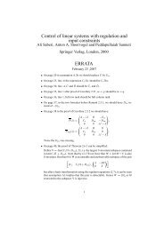
perform slightly better for <strong>order</strong>s p ≤ 8 <strong>in</strong> triangles. The distribution of these nodes <strong>in</strong><br />
the st<strong>and</strong>ard triangle is shown <strong>in</strong> Figure 1 for <strong>order</strong>s p = 2, 4, 6, 10. We also note that<br />
the nodal distributions <strong>in</strong> a triangle <strong>and</strong> tetrahedron with an L 2 -norm optimal Lebesgue<br />
constant were determ<strong>in</strong>ed <strong>in</strong> [7] <strong>and</strong> [8]. However, these nodes, <strong>in</strong> contrast with the Fekete<br />
<strong>and</strong> electrostatic po<strong>in</strong>ts, do not have an edge distribution which can be identified with<br />
Gauss-Lobatto-Jacobi po<strong>in</strong>ts. We refer to [25] for further overview on nodal (<strong>and</strong> modal)<br />
spectral/hp methods.<br />
To formulate the discont<strong>in</strong>uous Galerk<strong>in</strong> scheme, we first <strong>in</strong>troduce the local <strong>in</strong>ner<br />
product <strong>and</strong> its associated norm on Ω k as<br />
∫<br />
(u, v) Ω k = u · v dx, ‖u‖ 2 Ω<br />
= (u, u) k Ω k<br />
Ω k<br />
<strong>and</strong> on its boundary ∂Ω k as<br />
∫<br />
(u, v) ∂Ω k = u · v ds.<br />
∂Ω k<br />
We multiply (7) with the local test function φ ∈ Pp d(Ωk ), chosen to be the same <strong>in</strong>terpolat<strong>in</strong>g<br />
Lagrange polynomials L i (x) for the trial basis functions, drop the superscript k<br />
<strong>and</strong> <strong>in</strong>tegrate by parts over element Ω k to obta<strong>in</strong> the cont<strong>in</strong>uous weak formulation<br />
(<br />
Q ∂q )<br />
∂t , φ − (F,∇φ) Ω k = − (ˆn · F, φ) ∂Ω k , ∀Ω k ⊂ Ω K . (9)<br />
Ω k<br />
We then replace the cont<strong>in</strong>uous variable q with its discrete counterpart q N , <strong>and</strong> the<br />
exact flux F with the numerical flux ̂F to account for the multi-valued traces at the<br />
element boundary. F<strong>in</strong>ally, <strong>in</strong>tegration by parts for the second time results <strong>in</strong> the discrete<br />
formulation<br />
(<br />
Q ∂q N<br />
∂t<br />
) ( [<br />
+ ∇F N , φ = ˆn · F − ̂F<br />
] )<br />
, φ . (10)<br />
Ω k ∂Ω k<br />
6
The right-h<strong>and</strong> side of (10) is responsible for the communication between the elements<br />
through the numerical flux ̂F . The role of the numerical flux <strong>in</strong> the present spatial discretisation<br />
is discussed <strong>in</strong> [19] <strong>in</strong> the light of the Maxwell eigenvalue problem. Throughout this<br />
work, we use the upw<strong>in</strong>d flux [26], where <strong>in</strong>formation travels along local wave directions.<br />
In <strong>order</strong> to formulate the upw<strong>in</strong>d flux, we first <strong>in</strong>troduce the impedance Z <strong>and</strong> the<br />
conductance Y def<strong>in</strong>ed as<br />
Z = Y −1 = √ µ r /ε r .<br />
We also <strong>in</strong>troduce the associated quantities<br />
√<br />
Z ± = 1<br />
Y = µ ± r Z<br />
, ¯Z − + Z +<br />
= , Ȳ = Y − + Y +<br />
.<br />
± 2<br />
2<br />
ε ± r<br />
The upw<strong>in</strong>d flux at dielectric <strong>in</strong>terfaces then reads as<br />
ˆn · ̂F = 1 [ ( ¯Z−1 −ˆn × Z − H − N − ˆn × Z+ H + N + ˆn × ˆn × [E N ] ) ]<br />
2 Ȳ (ˆn −1 × Y − E − N + ˆn × Y + E + N + ˆn × ˆn × [H N ] ) , (11)<br />
where ( E − N , ) ( H− N <strong>and</strong> E<br />
+<br />
N , N) H+ denote the local <strong>and</strong> neighbour<strong>in</strong>g solution at the boundary<br />
of Ω k , respectively. We emphasise that the cross product is def<strong>in</strong>ed between vectors<br />
at each node of the element. For a detailed derivation of the upw<strong>in</strong>d flux we refer to [26].<br />
We should also recognise that<br />
[ ]<br />
−ˆn × H<br />
−<br />
N<br />
ˆn · F N =<br />
ˆn × E − ,<br />
N<br />
<strong>and</strong> comb<strong>in</strong><strong>in</strong>g this with (11), the penalis<strong>in</strong>g boundary term will now read<br />
(<br />
ˆn · F N − ̂F<br />
)<br />
= 1 [ ¯Z−1 (Z +ˆn ]<br />
× [[H N ]] − ˆn × ˆn × [[E N ]])<br />
2 Ȳ −1 (−Y +ˆn .<br />
× [[E N ]] − ˆn × ˆn × [[H N ]])<br />
To obta<strong>in</strong> the semi-discrete system we <strong>in</strong>troduce the N-by-N local mass <strong>and</strong> stiffness<br />
matrices as<br />
M ij = (L i (x), L j (x)) Ω k , S x ij = (L i(x), ∂ x L j (x)) Ω k , (12)<br />
S y ij = (L i(x), ∂ y L j (x)) Ω k , S z ij = (L i(x), ∂ z L j (x)) Ω k ,<br />
<strong>and</strong> the face-based mass matrices<br />
F il = (L i (x), L l (x)) ∂Ω k , (13)<br />
where the second <strong>in</strong>dex is limited to the boundaries of Ω k .<br />
We can now express the semi-discrete scheme as the follow<strong>in</strong>g system of ord<strong>in</strong>ary<br />
7
differential equations<br />
dE x N<br />
dt<br />
dE y N<br />
dt<br />
dE z N<br />
dt<br />
dH x N<br />
dt<br />
dH y N<br />
dt<br />
dH z N<br />
dt<br />
(<br />
) ∣<br />
x<br />
=(ε r M) −1 (S y HN z − Sz H y N ) + (ε rM) −1 F ˆn × Z+ [H N ] − ˆn × [E N ] ∣∣∣∣∂Ω<br />
,<br />
Z + + Z −<br />
k<br />
(<br />
=(ε r M) −1 (S z HN x − Sx HN z ) + (ε rM) −1 F<br />
(<br />
=(ε r M) −1 (S x H y N − Sy HN x ) + (ε rM) −1 F<br />
(<br />
=(ε r M) −1 (S z E y N − Sy EN z ) + (ε rM) −1 F<br />
) ∣<br />
y<br />
ˆn × Z+ [[H N ]] − ˆn × [[E N ]] ∣∣∣∣∂Ω<br />
,<br />
Z + + Z −<br />
k<br />
) ∣<br />
z<br />
ˆn × Z+ [H N ] − ˆn × [E N ] ∣∣∣∣∂Ω<br />
,<br />
Z + + Z −<br />
k<br />
(14)<br />
ˆn × Y ) ∣ + x<br />
[E N ] + ˆn × [[H N ]] ∣∣∣∣∂Ω<br />
,<br />
Y + + Y −<br />
k<br />
) ∣<br />
y ∣∣∣∣∂Ω<br />
,<br />
k<br />
(<br />
=(ε r M) −1 (S x EN z − S z EN) x + (ε r M) −1 F ˆn × Y + [[E N ]] + ˆn × [H N ]<br />
Y + + Y −<br />
(<br />
=(ε r M) −1 (S y EN x − S x E y N ) + (ε rM) −1 F ˆn × Y + [E N ] + ˆn × [[H N ]]<br />
Y + + Y −<br />
) ∣<br />
z ∣∣∣∣∂Ω<br />
.<br />
k<br />
(15)<br />
Here the fields EN x , Ey N , Ez N , Hx N , Hy N , <strong>and</strong> Hz N represent the discrete counterparts of<br />
scalar fields. That is the reason they are not typeset boldface, despite now be<strong>in</strong>g <strong>in</strong> fact<br />
vectors as a result of the discretisation. In contrast, we evaluate the numerical flux <strong>in</strong><br />
the right-h<strong>and</strong> side of (14)–(15) at each node at the boundary of the element us<strong>in</strong>g the<br />
discrete counterparts of vector fields. Then at each node the correspond<strong>in</strong>g component of<br />
the result<strong>in</strong>g vector is taken.<br />
The advantages of the above described discretisation are discussed <strong>in</strong> detail <strong>in</strong> [18] <strong>and</strong><br />
[35], where a number of numerical examples are also provided. Here it suffices to mention<br />
its optimal flexibility for mesh ref<strong>in</strong>ement, the possibility of <strong>in</strong>dependent adjustment of<br />
polynomial <strong>order</strong>s <strong>in</strong> each element (hp-adaptation), its excellent performance on parallel<br />
computers <strong>and</strong> that only matrix-matrix multiplications are needed dur<strong>in</strong>g the time <strong>in</strong>tegration.<br />
In this article, however, our aim is to analyse the properties of time -<strong>in</strong>tegration<br />
methods suitable for this spatial DG discretisation, therefore we assemble the local semidiscrete<br />
system (14)–(15) <strong>in</strong>to a global matrix <strong>and</strong> consider the ‘abstract’ semi-discrete<br />
system<br />
dq h<br />
dt<br />
= Aq h , (16)<br />
where A is the global matrix <strong>and</strong> q h = [E h , H h ] T represents the numerical approximation<br />
to the fields <strong>in</strong> the complete doma<strong>in</strong>. The matrix assembly is somewhat lengthy but<br />
straightforward, <strong>and</strong> it follows the st<strong>and</strong>ard procedure. See [25] for example.<br />
8
4 <strong>Runge</strong>-<strong>Kutta</strong> time-stepp<strong>in</strong>g methods<br />
From the po<strong>in</strong>t of view of time <strong>in</strong>tegration, one of the ma<strong>in</strong> difficulties <strong>in</strong> <strong>high</strong>-<strong>order</strong><br />
spectral/hp element methods is the restriction on the time step of explicit time-<strong>in</strong>tegration<br />
schemes. For hyperbolic systems <strong>in</strong> general, <strong>and</strong> for the advection equation <strong>in</strong> particular,<br />
it is known (see [25], for example) that the maximum eigenvalue of the semi-discrete global<br />
matrix grows as O(p 2 ) with polynomial <strong>order</strong> p, hence the time step is usually bounded<br />
by O(1/p 2 ). The time-step restriction then can generally be taken as<br />
∆t ≤ ∆t max = CFL(p) h k<br />
c k<br />
, (17)<br />
where h k is the m<strong>in</strong>imum edge length of all elements <strong>and</strong> c k is the maximum wave speed<br />
<strong>in</strong> the doma<strong>in</strong>. Here the parameter CFL depends on the degree of the polynomials used <strong>in</strong><br />
the spatial discretisation. If we apply any given time-<strong>in</strong>tegration scheme with fixed <strong>order</strong><br />
(i.e. <strong>in</strong>dependent of the polynomial <strong>order</strong> p) to the semi-discrete system (16), we have<br />
CFL(p) = C 1 p2, (18)<br />
where C is a constant, typically of <strong>order</strong> one. This condition may turn out to be rather<br />
restrictive as we go to <strong>high</strong>er <strong>and</strong> <strong>high</strong>er <strong>order</strong> approximations, even with a slightly <strong>in</strong>creas<strong>in</strong>g<br />
value for C (see Section 6).<br />
The low-storage <strong>Runge</strong>-<strong>Kutta</strong> schemes <strong>in</strong>troduced <strong>in</strong> [5] are among the most popular<br />
choices for time <strong>in</strong>tegration of the DG space-discretised Maxwell equations. Storage can<br />
be essential for large-scale computations <strong>and</strong> low-storage schemes require only two storage<br />
units per ODE variable. If we consider the ODE system<br />
du<br />
dt<br />
= L(u), (19)<br />
the general m-stage low-storage <strong>Runge</strong>-<strong>Kutta</strong> scheme [36, 5] can be written <strong>in</strong> the form<br />
u (0) = u n , v (0) = 0,<br />
v (i) = a i v (i−1) + ∆tL(u (i−1) ), i = 1, . . ., m, (20)<br />
u (i) = u (i−1) + b i v (i) , i = 1, . . ., m,<br />
u n+1 = u (m) ,<br />
where only u <strong>and</strong> an auxiliary variable v must be stored. The coefficients a i <strong>and</strong> b i have<br />
been determ<strong>in</strong>ed for a number of different low-storage <strong>Runge</strong>-<strong>Kutta</strong> schemes. See [5] <strong>and</strong><br />
[13] for more details. In this article we consider the fourth-<strong>order</strong> five-stage low-storage<br />
scheme also applied <strong>in</strong> [18]. The coefficients we use are listed <strong>in</strong> Table I.<br />
One possible way to achieve a weaker time-step restriction is the application of SSP-<br />
RK schemes. In [14] it was shown that for the l<strong>in</strong>ear autonomous system (19) the class<br />
9
of m-stage l<strong>in</strong>ear SSP-RK schemes, given recursively by<br />
u (0) = u n ,<br />
u (i) = u (i−1) + ∆tLu (i−1) , i = 1, . . .,m − 1 (21)<br />
u (m) =<br />
m−2<br />
∑<br />
k=0<br />
u n+1 = u (m)<br />
where α 1,0 = 1 <strong>and</strong><br />
α m,k u (k) + α m,m−1<br />
(<br />
u (m−1) + ∆tLu (m−1)) ,<br />
α m,k = 1 k α m−1,k−1, k = 1, . . ., m − 2<br />
α m,m−1 = 1 m! ,<br />
α m,0 = 1 −<br />
m−1<br />
∑<br />
α m,k ,<br />
k=1<br />
are mth-<strong>order</strong> accurate. This was extended to l<strong>in</strong>ear non-autonomous systems by Chen<br />
et al. [6]. In that work the authors demonstrated that when applied together with the<br />
classical discont<strong>in</strong>uous Galerk<strong>in</strong> method [9, 11], the SSP-RK scheme gives (p + 1)st-<strong>order</strong><br />
convergence with the stability bound<br />
CFL(p) = C 1<br />
2p + 1<br />
(22)<br />
with C = 1, as long as for a given spatial discretisation of polynomial <strong>order</strong> p, the<br />
correspond<strong>in</strong>g SSP-RK method has <strong>order</strong> p + 1. The stability regions of several SSP-RK<br />
methods <strong>and</strong> the low-storage five-stage fourth-<strong>order</strong> <strong>Runge</strong>-<strong>Kutta</strong> method are displayed<br />
<strong>in</strong> Figure 2.<br />
5 Analysis of the dispersion <strong>and</strong> <strong>dissipation</strong> <strong>error</strong><br />
A critical factor <strong>in</strong> the numerical simulation of wave-propagation is the artificial <strong>dissipation</strong><br />
<strong>and</strong>/or dispersion <strong>in</strong>flicted on the waves due to numerical discretisation <strong>error</strong>s. In<br />
<strong>order</strong> to analyse these properties of the different schemes, we resort to the one-dimensional<br />
<strong>and</strong> two-dimensional forms of the Maxwell equations with periodic boundary conditions.<br />
First, these reduced models are formulated <strong>and</strong> then we perform a numerical Fourier<br />
analysis of the fully discrete schemes to <strong>in</strong>vestigate the dispersion <strong>and</strong> <strong>dissipation</strong> <strong>error</strong>s<br />
as a function of mesh size per wave length <strong>and</strong> time step. This analysis provides important<br />
<strong>in</strong>formation on the accuracy of the schemes regard<strong>in</strong>g wave motion <strong>and</strong> the relation<br />
between time step, mesh size <strong>and</strong> polynomial <strong>order</strong>.<br />
5.1 Wave equation <strong>in</strong> one <strong>and</strong> two dimensions<br />
The Maxwell equations <strong>in</strong> one dimension read<br />
ε r<br />
∂E<br />
∂t = −∂H ∂x ,<br />
µ ∂H<br />
r<br />
∂t = −∂E ∂x , (23)<br />
10
or they can be expressed by the wave equation<br />
∂ 2 E<br />
∂t 2 − 1<br />
ε r µ r<br />
∂ 2 E<br />
∂x 2 = 0,<br />
<strong>in</strong> the doma<strong>in</strong> Ω ⊂ R. In conservative form (7), this reads<br />
with<br />
Q ∂q<br />
∂t<br />
+ ∇ · F (q) = 0 (24)<br />
Q = diag(ε r , µ r ), q =<br />
[ [ E H<br />
, F (q) = .<br />
H]<br />
E]<br />
For the two-dimensional analysis we take the transverse magnetic (TM) polarisation of<br />
the Maxwell equations<br />
∂H x<br />
µ r<br />
∂t<br />
∂H y<br />
µ r<br />
∂t<br />
∂E z<br />
ε r<br />
∂t<br />
= − ∂Ez<br />
∂y ,<br />
= ∂Ez<br />
∂x ,<br />
= ∂Hy<br />
∂x − ∂Hx<br />
∂y ,<br />
which is aga<strong>in</strong> equivalent to the second-<strong>order</strong> wave equation,<br />
∂ 2 E z<br />
∂t 2 − 1<br />
ε r µ r<br />
∇ 2 E z = 0.<br />
Thus we arrive at the first-<strong>order</strong> system (7)<br />
with<br />
Q ∂q<br />
∂t<br />
+ ∇ · F (q) = 0, (25)<br />
⎡ ⎤ ⎡ ⎤<br />
H x<br />
0 −E z<br />
Q = diag(µ r , µ r , ε r ), q = ⎣H y ⎦, F(q) = ⎣E z 0 ⎦.<br />
E z H y −H x<br />
5.2 <strong>Dispersion</strong> <strong>and</strong> <strong>dissipation</strong> analysis of the global scheme<br />
For the analysis of the fully discrete schemes, we consider (24) <strong>and</strong> (25) <strong>in</strong> the doma<strong>in</strong>s<br />
Ω = [−1, 1] <strong>and</strong> Ω = [−1, 1] 2 , respectively. Furthermore, we use uniform meshes <strong>and</strong><br />
assume that the boundaries are periodic.<br />
11
5.2.1 One-dimensional Fourier analysis<br />
We are primarily <strong>in</strong>terested <strong>in</strong> wave propagation <strong>and</strong> <strong>in</strong> the associated dispersion <strong>and</strong><br />
<strong>dissipation</strong> <strong>error</strong> of the RKDG scheme. We consider the one-dimensional semi-discrete<br />
scheme (16)<br />
dq h<br />
dt<br />
= Aq h<br />
<strong>in</strong> the doma<strong>in</strong> Ω = [−1, 1] filled with vacuum (or air) <strong>and</strong> assume a monochromatic plane<br />
wave (which is also a Fourier mode)<br />
q h (0) = q 0 h = [ ]<br />
e ikx h<br />
, e ikx h T<br />
as <strong>in</strong>itial condition. Here, x h represents the vector of the nodes used for the spatial<br />
discretisation. We denote the angular wave frequency with ω. The exact wave number<br />
k is given by the dispersion relation k 2 = ω 2 /c 2 , with c be<strong>in</strong>g the speed of light. The<br />
time-exact discrete Fourier mode at time level t n = n∆t will read<br />
q h (n∆t) = ν n q h (0) = e −iωn∆t [ e ikx h<br />
, e ikx h] T<br />
(26)<br />
with exact amplification factor ν n = e −iωn∆t <strong>and</strong> i 2 = −1. To see the effect of the timestepp<strong>in</strong>g<br />
method, we replace the exact amplification factor ν n with its discrete counterpart<br />
νh n <strong>and</strong> take the fully discrete Fourier mode as<br />
q n h = νn h q0 h = νn h<br />
[ ]<br />
e<br />
ikx h<br />
, e ikx h T<br />
. (27)<br />
In addition, we write the SSP-RK scheme as a two-level explicit scheme. Thus<br />
q n+1<br />
h<br />
= Bq n h (28)<br />
holds with amplification matrix<br />
B =<br />
m∑<br />
l=0<br />
1<br />
l! (∆tA)l (29)<br />
<strong>and</strong> with m be<strong>in</strong>g the <strong>order</strong> of the SSP-RK time-stepp<strong>in</strong>g scheme. Substitut<strong>in</strong>g (27) <strong>in</strong>to<br />
(28) results <strong>in</strong> the equation<br />
[ ]<br />
ν n+1<br />
h e<br />
ikx h<br />
, e ikx h T [ ]<br />
= Bν<br />
n<br />
h e<br />
ikx h<br />
, e ikx h T<br />
,<br />
which, after division with νh n , reduce to the eigenvalue problem<br />
ν h q 0 h = Bq 0 h. (30)<br />
Solv<strong>in</strong>g this eigenvalue equation will produce p + 1 different values for ν h,j (<strong>and</strong> as many<br />
correspond<strong>in</strong>g eigenvectors q 0 h,j ). Bear<strong>in</strong>g <strong>in</strong> m<strong>in</strong>d that<br />
ν h,j = e −i˜ω h,j∆t ,<br />
12
with complex numerical frequencies ˜ω h,j , we can establish the dispersion <strong>and</strong> <strong>dissipation</strong><br />
properties of the scheme. For that, we consider the real (for dispersion) <strong>and</strong> imag<strong>in</strong>ary<br />
(for <strong>dissipation</strong>) parts of the complex numerical frequencies ˜ω h,j = (i/∆t) ln ν h,j , that is<br />
ω h,j = Re [˜ω h,j ] = Re [(i/∆t) ln ν h,j ], ρ h,j = Im [˜ω h,j ] = Im [(i/∆t) ln ν h,j ] ,<br />
with real numerical frequency ω h,j <strong>and</strong> numerical <strong>dissipation</strong> ρ h,j , both correspond<strong>in</strong>g to<br />
the eigenvalue ν h,j . One of the computed modes will be close to the frequency of the<br />
physical mode. This represents the approximation properties of our scheme. The other<br />
modes are spurious. To decide which eigenvalue should be considered, we def<strong>in</strong>e the<br />
<strong>dissipation</strong> <strong>error</strong> as err diss<br />
h,j = |ρ h,j | − 1 <strong>and</strong> the dispersion <strong>error</strong> as the absolute value of<br />
dispersion <strong>error</strong> err disp<br />
h,j<br />
= |ω − ω h,j |. The numerical Fourier mode is now taken as the<br />
closest eigenvalue to the physical mode<br />
{ √ }<br />
( ) 2 ( )<br />
ν h := ν h,j : m<strong>in</strong> err disp<br />
j<br />
h,j + err<br />
diss 2<br />
h,j<br />
. (31)<br />
In the numerical dispersion <strong>and</strong> <strong>dissipation</strong> analysis of the fully discrete schemes, we<br />
consider a wide range of values for ∆t <strong>and</strong> h k . The eigenvalues of (30) are computed <strong>in</strong><br />
Matlab.<br />
It is also important to consider the convergence of the numerical dispersion <strong>and</strong> <strong>dissipation</strong><br />
<strong>error</strong>. In [1] a complete dispersion <strong>and</strong> <strong>dissipation</strong> analysis of the semi-discrete<br />
advection equation was carried out for discont<strong>in</strong>uous Galerk<strong>in</strong> methods with <strong>high</strong>-<strong>order</strong><br />
tensor-product elements. In that article it was proven that <strong>in</strong> the asymptotic region<br />
hk = 2πh → 0 (with λ be<strong>in</strong>g the wave length) the dispersion relation for a pth-<strong>order</strong><br />
λ<br />
method is accurate to <strong>order</strong> 2p + 3 for the dispersion <strong>error</strong> <strong>and</strong> <strong>order</strong> 2p + 2 for the <strong>dissipation</strong><br />
<strong>error</strong>. See [22] <strong>and</strong> [1] for more details. In a more recent work [2] the dispersion<br />
<strong>and</strong> <strong>dissipation</strong> analysis of the semi-discrete wave equation was provided for some low<strong>order</strong><br />
schemes (l<strong>in</strong>ear elements for the general DG <strong>and</strong> up to third <strong>order</strong> elements for the<br />
IP-DG) <strong>and</strong> the authors also conjectured on how the results would extend to arbitrary<br />
<strong>order</strong> elements. For the fully discrete system we consider here, the rate of convergence<br />
is also <strong>in</strong>fluenced by the time-stepp<strong>in</strong>g method. However, for most polynomial <strong>order</strong>s p,<br />
the convergence of the dispersion <strong>and</strong> <strong>dissipation</strong> <strong>error</strong> still by far supersedes that of the<br />
<strong>error</strong> measured <strong>in</strong> the l 2 -norm. The numerical results are discussed <strong>in</strong> Section 6.<br />
5.2.2 Two-dimensional Fourier analysis<br />
As <strong>in</strong> one dimension, we assemble our right-h<strong>and</strong> side <strong>in</strong>to a global matrix <strong>and</strong> consider<br />
the abstract Cauchy problem (16)<br />
dq h<br />
dt<br />
= Aq h<br />
where now q = [H x h , Hy h , Ez h ]T <strong>and</strong> the matrix A represents the semi-discrete system result<strong>in</strong>g<br />
from the discretisation of (25). The only difference <strong>in</strong> the mathematical formulation<br />
to the one-dimensional case is that the dispersion relation now reads k 2 x + k 2 y = ω 2 /c 2 .<br />
The time-exact discrete Fourier mode satisfy<strong>in</strong>g (25) is equal to<br />
q n h = νn [ (k y /ω)e ikxx h+ik yy h<br />
, (−k x /ω)e ikxx h+ik yy h<br />
, e ikxx h+ik yy h<br />
] T<br />
(32)<br />
13
<strong>in</strong> the two-dimensional doma<strong>in</strong> Ω = [−1, 1] 2 . From here we follow exactly the same<br />
l<strong>in</strong>e as <strong>in</strong> the one-dimensional case. As <strong>in</strong>itial condition we take a monochromatic plane<br />
wave with different wave numbers k y <strong>and</strong> k x between which the relation k y = 2k x always<br />
holds. This represents a monochromatic plane wave travell<strong>in</strong>g at an angle of about 26.565 ◦<br />
aga<strong>in</strong>st the x axis. As <strong>in</strong> one dimension, a range of values of ∆t <strong>and</strong> h k are considered.<br />
We note that for comput<strong>in</strong>g the matrix exponential <strong>in</strong> (29) the simple Horner’s rule is<br />
applied (see [12] for example).<br />
6 Numerical results<br />
6.1 One-dimensional cavity<br />
In <strong>order</strong> to <strong>in</strong>vestigate if the SSP-RK scheme reta<strong>in</strong>s the <strong>high</strong>-<strong>order</strong> convergence of the<br />
spatial discretisation [18], we consider the one-dimensional cavity problem <strong>in</strong> the doma<strong>in</strong><br />
x ∈ [−1, 1], with two different non-magnetic (µ r,1 = µ r,2 = 1) materials. The material<br />
<strong>in</strong>terface is situated at x = 0 <strong>and</strong> the two different materials have a relative permittivity<br />
of ε r,1 = 1 <strong>and</strong> ε r,2 = 2.25, respectively. The <strong>error</strong> is measured aga<strong>in</strong>st the exact solution,<br />
which is <strong>in</strong>cluded <strong>in</strong> the Appendix. We set the frequency of the wave at ω = 2π, the same<br />
throughout the whole doma<strong>in</strong>, which entails the correspond<strong>in</strong>g wave numbers k 1 = 2π<br />
<strong>and</strong> k 2 = 3π, respectively. In Table II we show the l 2 -<strong>error</strong> ‖q N − q exact ‖ at f<strong>in</strong>al time<br />
T = 1 for different <strong>order</strong>s of the local polynomials. For the time <strong>in</strong>tegration, we use the<br />
(p + 1)st-<strong>order</strong> SSP-RK method (4) with correspond<strong>in</strong>g maximum time step (22). We<br />
can see that <strong>in</strong> the asymptotic region hk ≪ 1, (p + 1)st-<strong>order</strong> convergence is achieved for<br />
polynomial <strong>order</strong>s p <strong>in</strong> the range of 1 ≤ p ≤ 9.<br />
In the next example we compare the performance of the two different time-<strong>in</strong>tegration<br />
schemes def<strong>in</strong>ed <strong>in</strong> Section 4. We also <strong>in</strong>clude the ubiquitous st<strong>and</strong>ard fourth-<strong>order</strong> RK<br />
scheme as a reference. The constant <strong>in</strong> the time-step restriction (22) of the SSP-RK<br />
schemes is set to C = 1 for all values of polynomial <strong>order</strong> p. For the low-storage <strong>Runge</strong>-<br />
<strong>Kutta</strong> scheme <strong>and</strong> the st<strong>and</strong>ard <strong>Runge</strong>-<strong>Kutta</strong> scheme, we use the value C = 1 <strong>in</strong> (18)<br />
for p ≤ 5, <strong>and</strong> the value C = 2 when 5 < p ≤ 10. We consider the same cavity, but<br />
now filled with vacuum (or air) <strong>and</strong> <strong>in</strong>tegrate for a relatively long time, until T = 1000<br />
time periods. The results are shown <strong>in</strong> Table III for different <strong>order</strong>s <strong>and</strong> different number<br />
of elements. We measure the computational work as the number of operations, which is<br />
simply computed as<br />
ops = N T m,<br />
where N T is the number of time steps needed until f<strong>in</strong>al time T, <strong>and</strong> m represents the<br />
number of stages <strong>in</strong> a given RK scheme. For each RK scheme we use the correspond<strong>in</strong>g<br />
maximum time step def<strong>in</strong>ed <strong>in</strong> Section 4. The test was carried out for <strong>order</strong>s p = 3, p = 6<br />
<strong>and</strong> p = 10. Significant differences <strong>in</strong> accuracy, up to O(4), occur between the schemes for<br />
<strong>order</strong>s p = 6 <strong>and</strong> p = 10. For each <strong>order</strong>, we <strong>in</strong>clude two subtables, one for a relatively f<strong>in</strong>e<br />
spatial grid <strong>and</strong> one for a comparatively coarse one. The most favourable characteristic<br />
of the SSP-RK schemes is that the better accuracy occurs without significant–or <strong>in</strong>deed,<br />
any–<strong>in</strong>crease <strong>in</strong> the number of operations.<br />
14
Perhaps even more illum<strong>in</strong>at<strong>in</strong>g is to see how much computational work is needed to<br />
obta<strong>in</strong> a given accuracy. In Table IV we show the number of operations necessary to<br />
achieve the <strong>error</strong> l 2 err = 10−5 at f<strong>in</strong>al time T = 1000. The comparisons of the different<br />
time-<strong>in</strong>tegration schemes are made for fixed polynomial <strong>order</strong> <strong>and</strong> spatial mesh, so that<br />
only the time step was lowered <strong>in</strong> <strong>order</strong> to decrease the <strong>error</strong>s.<br />
6.2 Numerical dispersion <strong>and</strong> <strong>dissipation</strong> <strong>error</strong><br />
To conduct the dispersion <strong>and</strong> <strong>dissipation</strong> analysis described <strong>in</strong> Section 5, we carry out two<br />
types of experiments. First, we consider the convergence of the dispersion <strong>and</strong> <strong>dissipation</strong><br />
<strong>error</strong>s <strong>in</strong> one dimension. The polynomials we apply for the spatial discretisation range<br />
from p = 1 to p = 10, <strong>and</strong> for the time discretisation we use the correspond<strong>in</strong>g (p + 1)st<strong>order</strong><br />
SSP-RK scheme (4) with maximum time step (22). Because the actual <strong>error</strong>s may<br />
be rather small for large values of p, we <strong>in</strong>crease the wave number (thus decrease the wave<br />
length) for <strong>high</strong>er-<strong>order</strong> polynomials. Consequently, the follow<strong>in</strong>g wave numbers are used<br />
<strong>in</strong> our one-dimensional Fourier analysis:<br />
⎧<br />
π if p = 1, 2,<br />
⎪⎨<br />
2π if p = 3, 4,<br />
k =<br />
4π if p = 5, 6, 7,<br />
⎪⎩<br />
8π if p = 8, 9, 10.<br />
The <strong>error</strong>s, def<strong>in</strong>ed <strong>in</strong> Section 5, <strong>and</strong> the rate of the convergence are shown <strong>in</strong> Table V<br />
for the dispersion <strong>and</strong> <strong>in</strong> Table VI for the <strong>dissipation</strong>. Although we cannot establish<br />
precise convergence rates due the <strong>in</strong>fluence of the time discretisation on the dispersion<br />
<strong>and</strong> <strong>dissipation</strong> properties, an <strong>order</strong> of convergence of approximately 2p is achieved for<br />
both the <strong>dissipation</strong> <strong>and</strong> dispersion <strong>error</strong>. Compar<strong>in</strong>g these results to the f<strong>in</strong>d<strong>in</strong>gs of [1]<br />
<strong>and</strong> [2] already implies that the SSP-RK time <strong>in</strong>tegration has a less dom<strong>in</strong>ant effect on<br />
the dispersion <strong>and</strong> <strong>dissipation</strong> <strong>error</strong>s.<br />
In the second experiment, we consider a wide range of time steps ∆t <strong>and</strong> mesh sizes<br />
h, <strong>and</strong> exam<strong>in</strong>e the dispersion <strong>and</strong> <strong>dissipation</strong> <strong>error</strong>s of the schemes as a function of wave<br />
length per mesh size (λ/h), degrees of freedom per wave length (DoF/λ) <strong>and</strong> relative time<br />
step (∆t/∆t max ). The value ∆t/∆t max = 1 <strong>in</strong>dicates the size of the maximum time step,<br />
def<strong>in</strong>ed as <strong>in</strong> (22) <strong>in</strong> Section 4. The contour plots of the dispersion <strong>error</strong> (or dispersion<br />
<strong>error</strong>) for the one-dimensional analysis with wave number k = 2π is shown <strong>in</strong> Figure 3<br />
for <strong>order</strong>s p = 1, 2. The same plots for the <strong>dissipation</strong> <strong>error</strong> are displayed <strong>in</strong> Figure 4.<br />
For this range of values the dispersion <strong>error</strong> is generally at least one <strong>order</strong> <strong>high</strong>er than<br />
the <strong>dissipation</strong> <strong>error</strong>, <strong>and</strong> it can be improved by both tak<strong>in</strong>g smaller time steps <strong>and</strong>/or<br />
ref<strong>in</strong><strong>in</strong>g the spatial grid.<br />
We carry out the same experiment <strong>in</strong> two dimensions on a uniform grid with wave<br />
numbers k x = π <strong>and</strong> k y = 2π for <strong>order</strong>s p = 1, 2, 3, 4, 5 <strong>and</strong> k x = 2π <strong>and</strong> k y = 4π for<br />
<strong>order</strong> p = 6. The number of elements used to construct the uniform meshes range from<br />
200 elements to 8 elements for p = 1, 2, 3, 4; from 128 elements to 8 elements for p = 5;<br />
<strong>and</strong> from 72 elements to 8 elements for p = 6. The contour plots of the dispersion <strong>and</strong><br />
<strong>dissipation</strong> <strong>error</strong>s are shown <strong>in</strong> Figure 5 <strong>and</strong> <strong>in</strong> Figure 6, respectively. Note that the<br />
15
studied range of wave lengths per mesh size differs significantly from that of the onedimensional<br />
case <strong>and</strong> occasionally from one another. It can be deduced that the spatial<br />
discretisation dom<strong>in</strong>ates the dispersion <strong>error</strong>, which is all the more relevant because the<br />
dispersion <strong>error</strong> is at least one <strong>order</strong> <strong>high</strong>er than the <strong>dissipation</strong> <strong>error</strong> for all polynomial<br />
<strong>order</strong>s considered. Another important feature–shown <strong>in</strong> Figure 9–is the decreas<strong>in</strong>g number<br />
of degrees of freedom needed to obta<strong>in</strong> a given accuracy as we go to <strong>high</strong>er-<strong>order</strong> elements.<br />
For <strong>in</strong>stance, to atta<strong>in</strong> a dispersion <strong>error</strong> of 10 −3 , we need about 14-15 degrees of freedom<br />
per wave length for discretisation with second-<strong>order</strong> polynomials <strong>and</strong> about six for the<br />
discretisation with sixth-<strong>order</strong> polynomials.<br />
One of the ma<strong>in</strong> advantages of DG methods is that they are relatively <strong>in</strong>sensitive to<br />
the uniformity of the mesh from the po<strong>in</strong>t of view of accuracy <strong>and</strong> convergence. In <strong>order</strong><br />
to illustrate that this is the case for the dispersion <strong>and</strong> <strong>dissipation</strong> behaviour as well, we<br />
perform the same two-dimensional analysis on non-uniform r<strong>and</strong>om meshes. To construct<br />
the non-uniform mesh we r<strong>and</strong>omly relocate all <strong>in</strong>ner (ie. not ly<strong>in</strong>g on the boundary)<br />
vertices of the uniform mesh with<strong>in</strong> the range [− h ed<br />
3<br />
, h ed<br />
3<br />
] <strong>in</strong> both directions, where h ed<br />
is length of the uniformly distributed (one-dimensional) ‘boundary’ elements. S<strong>in</strong>ce the<br />
total number of elements <strong>in</strong> the non-uniform mesh is the same as <strong>in</strong> the uniform mesh, the<br />
values DoF/λ should also be the same (because this is the case ‘on average’). However,<br />
on the bottom axes the smallest value of h is taken for comput<strong>in</strong>g λ/h. The results<br />
are shown <strong>in</strong> Figure 7 for the dispersion <strong>error</strong> <strong>and</strong> <strong>in</strong> Figure 8 for the <strong>dissipation</strong> <strong>error</strong>.<br />
They are qualitatively the same as the correspond<strong>in</strong>g results on uniform meshes, which<br />
demonstrates the robustness of the RKDG method.<br />
7 Conclusion<br />
The ma<strong>in</strong> purpose of this article has been to study the global dispersion <strong>and</strong> <strong>dissipation</strong><br />
<strong>error</strong>s of a <strong>high</strong>-<strong>order</strong> DG spectral element discretisation comb<strong>in</strong>ed with the <strong>high</strong>-<strong>order</strong><br />
SSP-RK time <strong>in</strong>tegration. We have shown that by apply<strong>in</strong>g the (p + 1)st-<strong>order</strong> SSP-<br />
RK scheme to a spatial discretisation with pth-<strong>order</strong> polynomials we can reta<strong>in</strong> (p +<br />
1)st-<strong>order</strong> convergence (without preprocess<strong>in</strong>g) <strong>in</strong> the l 2 -norm. Even when the <strong>order</strong><br />
of the discretisation is <strong>in</strong>creased beyond the accuracy of the fixed-<strong>order</strong> schemes, the<br />
computational work for the SSP-RK scheme is not significantly <strong>high</strong>er than that of the<br />
fixed-<strong>order</strong> ones. This favourable property can be expla<strong>in</strong>ed by the much looser time-step<br />
restriction. It should be noted, however, that for large systems, the SSP-RK schemes could<br />
have a major disadvantage over low-storage RK schemes due to storage requirements. This<br />
is because an m-stage SSP-RK scheme requires m storage units per time step, whereas a<br />
low storage scheme requires only two storage units per time step.<br />
Through numerical Fourier analysis, it has been demonstrated that the dispersion<br />
<strong>error</strong> of the global scheme is generally at least one <strong>order</strong> <strong>high</strong>er than the <strong>dissipation</strong> <strong>error</strong>,<br />
irrespective of the actual <strong>order</strong> of the discretisation. It has also turned out that with<strong>in</strong> the<br />
studied range of mesh sizes h <strong>and</strong> time steps ∆t we cannot ga<strong>in</strong> anyth<strong>in</strong>g on the dispersion<br />
<strong>error</strong> by decreas<strong>in</strong>g the time step, i.e. it is worth us<strong>in</strong>g the largest one permitted by the<br />
CFL condition. This seem<strong>in</strong>gly unusual property can be expla<strong>in</strong>ed by the fact that the<br />
maximum time step allowed by the CFL condition already <strong>in</strong>flicts a far smaller dispersion<br />
<strong>error</strong> than that of the space discretisation. Us<strong>in</strong>g this condition it has also been shown<br />
16
that the convergence rate of the dispersion <strong>and</strong> <strong>dissipation</strong> <strong>error</strong> is far <strong>high</strong>er, namely<br />
O(2p), than that of the <strong>error</strong> measured <strong>in</strong> the l 2 -norm. Another important feature of the<br />
global scheme is that the number of degrees of freedom to obta<strong>in</strong> a given accuracy also<br />
decreases as the <strong>order</strong> of the approximation grows.<br />
Appendix<br />
The exact solution to (23) <strong>in</strong> the one-dimensional metallic cavity described <strong>in</strong> Section<br />
6.1–with κ = 1, 2 signify<strong>in</strong>g the two regions filled with different materials–is given by<br />
where<br />
<strong>and</strong><br />
E κ = [ −A κ e <strong>in</strong>κωx + B κ e −<strong>in</strong>κωx] e iωt ,<br />
H κ = [ A κ e <strong>in</strong>κωx + B κ e −<strong>in</strong>κωx] e iωt ,<br />
A 1 = n 2 cos(n 2 ω)<br />
n 1 cos(n 1 ω) , A 2 = e −iω(n 1+n 2 ) ,<br />
B 1 = A 1 e −i2n 1ω , B 2 = A 2 e i2n 2ω .<br />
Here n κ = √ ε κ represents the local <strong>in</strong>dex of refraction, <strong>and</strong> the frequency takes the value<br />
ω = 2π/n if n 1 = n 2 = n or is found as the solution to the equation<br />
−n 2 tan(n 1 ω) = n 1 tan(n 2 ω).<br />
References<br />
[1] M. A<strong>in</strong>sworth. Dispersive <strong>and</strong> dissipative behaviour of <strong>high</strong> <strong>order</strong> discont<strong>in</strong>uous<br />
Galerk<strong>in</strong> f<strong>in</strong>ite element methods. J. Comput. Phys., 198(1):106–130, 2004.<br />
[2] M. A<strong>in</strong>sworth, P. Monk, <strong>and</strong> W. Muniz. Dispersive <strong>and</strong> dissipative properties of<br />
discont<strong>in</strong>uous Galerk<strong>in</strong> f<strong>in</strong>ite element methods for the second-<strong>order</strong> wave equation.<br />
J. Sci. Comput., 27:5–40, 2006.<br />
[3] A. Bossavit. A rationale for ‘edge-elements’ <strong>in</strong> 3-D fields computations. IEEE Trans.<br />
Magn., 24(1):74–79, 1988.<br />
[4] A. Bossavit. Solv<strong>in</strong>g Maxwell equations <strong>in</strong> a closed cavity, <strong>and</strong> the question of ‘spurious<br />
modes’. IEEE Trans. Magn., 26(2):702–705, 1990.<br />
[5] M. H. Carpenter <strong>and</strong> C. A. Kennedy. Fourth <strong>order</strong> 2N-storage <strong>Runge</strong>-<strong>Kutta</strong> scheme,<br />
NASA-TM-109112 (NASA Langley Research Center, VA, 1994).<br />
[6] M.-H. Chen, B. Cockburn, <strong>and</strong> F. Reitich. High-<strong>order</strong> RKDG methods for computational<br />
electromagnetics. J. Sci. Comput., 22/23:205–226, 2005.<br />
17
[7] Q. Chen <strong>and</strong> I. Babuška. Approximate optimal po<strong>in</strong>ts for polynomial <strong>in</strong>terpolation of<br />
real functions <strong>in</strong> an <strong>in</strong>terval <strong>and</strong> <strong>in</strong> a triangle. Comput. Methods Appl. Mech. Engrg.,<br />
128(3-4):405–417, 1995.<br />
[8] Q. Chen <strong>and</strong> I. Babuška. The optimal symmetrical po<strong>in</strong>ts for polynomial <strong>in</strong>terpolation<br />
of real functions <strong>in</strong> the tetrahedron. Comput. Methods Appl. Mech. Engrg.,<br />
137(1):89–94, 1996.<br />
[9] B. Cockburn, G. E. Karniadakis, <strong>and</strong> C.-W. Shu. The development of discont<strong>in</strong>uous<br />
Galerk<strong>in</strong> methods. In Discont<strong>in</strong>uous Galerk<strong>in</strong> methods (Newport, RI, 1999),<br />
volume 11 of Lect. Notes Comput. Sci. Eng., pages 3–50. Spr<strong>in</strong>ger, Berl<strong>in</strong>, 2000.<br />
[10] B. Cockburn, F. Li, <strong>and</strong> C.-W. Shu. Locally divergence-free discont<strong>in</strong>uous Galerk<strong>in</strong><br />
methods for the Maxwell equations. J. Comput. Phys., 194(2):588–610, 2004.<br />
[11] B. Cockburn <strong>and</strong> C.-W. Shu. <strong>Runge</strong>-<strong>Kutta</strong> discont<strong>in</strong>uous Galerk<strong>in</strong> methods for<br />
convection-dom<strong>in</strong>ated problems. J. Sci. Comput., 16(3):173–261, 2001.<br />
[12] G. H. Golub <strong>and</strong> C. F. Van Loan. Matrix computations. Johns Hopk<strong>in</strong>s Studies <strong>in</strong><br />
the Mathematical Sciences. Johns Hopk<strong>in</strong>s University Press, Baltimore, MD, third<br />
edition, 1996.<br />
[13] S. Gottlieb <strong>and</strong> C.-W. Shu. Total variation dim<strong>in</strong>ish<strong>in</strong>g <strong>Runge</strong>-<strong>Kutta</strong> schemes. Math.<br />
Comp., 67(221):73–85, 1998.<br />
[14] S. Gottlieb, C.-W. Shu, <strong>and</strong> E. Tadmor. Strong stability-preserv<strong>in</strong>g <strong>high</strong>-<strong>order</strong> time<br />
discretization methods. SIAM Rev., 43(1):89–112, 2001.<br />
[15] J. S. Hesthaven. From electrostatics to almost optimal nodal sets for polynomial<br />
<strong>in</strong>terpolation <strong>in</strong> a simplex. SIAM J. Numer. Anal., 35(2):655–676, 1998.<br />
[16] J. S. Hesthaven. High-<strong>order</strong> accurate methods <strong>in</strong> time-doma<strong>in</strong> computational electromagnetics.<br />
A review. Advances <strong>in</strong> Imag<strong>in</strong>g <strong>and</strong> Electron Physics, 127(1):59–123,<br />
2003.<br />
[17] J. S. Hesthaven <strong>and</strong> C. H. Teng. Stable spectral methods on tetrahedral elements.<br />
SIAM J. Sci. Comput., 21(6):2352–2380, 2000.<br />
[18] J. S. Hesthaven <strong>and</strong> T. Warburton. Nodal <strong>high</strong>-<strong>order</strong> methods on unstructured grids.<br />
I. Time-doma<strong>in</strong> solution of Maxwell’s equations. J. Comput. Phys., 181(1):186–221,<br />
2002.<br />
[19] J. S. Hesthaven <strong>and</strong> T. Warburton. High-<strong>order</strong> nodal discont<strong>in</strong>uous Galerk<strong>in</strong> methods<br />
for the Maxwell eigenvalue problem. Philos. Trans. R. Soc. Lond. Ser. A Math. Phys.<br />
Eng. Sci., 362(1816):493–524, 2004.<br />
[20] R. Hiptmair. F<strong>in</strong>ite elements <strong>in</strong> computational electromagnetism. Acta Numer.,<br />
11:237–339, 2002.<br />
[21] P. Houston, I. Perugia, <strong>and</strong> D. Schötzau. Mixed discont<strong>in</strong>uous Galerk<strong>in</strong> approximation<br />
of the Maxwell operator. SIAM J. Numer. Anal., 42(1):434–459, 2004.<br />
18
[22] F. Q. Hu <strong>and</strong> H. L. Atk<strong>in</strong>s. Eigensolution analysis of the discont<strong>in</strong>uous Galerk<strong>in</strong><br />
method with nonuniform grids. I. One space dimension. J. Comput. Phys.,<br />
182(2):516–545, 2002.<br />
[23] F. Q. Hu, M. Y. Hussa<strong>in</strong>i, <strong>and</strong> P. Rasetar<strong>in</strong>era. An analysis of the discont<strong>in</strong>uous<br />
Galerk<strong>in</strong> method for wave propagation problems. J. Comput. Phys., 151(2):921–946,<br />
1999.<br />
[24] J. J<strong>in</strong>. The f<strong>in</strong>ite element method <strong>in</strong> electromagnetics. Wiley-Interscience [John Wiley<br />
& Sons], New York, second edition, 2002.<br />
[25] G. E. Karniadakis <strong>and</strong> S. J. Sherw<strong>in</strong>. Spectral/hp element methods for computational<br />
fluid dynamics. Numerical Mathematics <strong>and</strong> Scientific Computation. Oxford<br />
University Press, New York, second edition, 2005.<br />
[26] A. H. Mohammadian, V. Shankar, <strong>and</strong> W. F. Hall. Computation of electromagnetic<br />
scatter<strong>in</strong>g <strong>and</strong> radiation us<strong>in</strong>g a time-doma<strong>in</strong> f<strong>in</strong>ite-volume discretization procedure.<br />
Computer Physics Communications, 68:175–196, Nov. 1991.<br />
[27] P. Monk. F<strong>in</strong>ite element methods for Maxwell’s equations. Numerical Mathematics<br />
<strong>and</strong> Scientific Computation. Oxford University Press, New York, 2003.<br />
[28] P. Monk <strong>and</strong> G. R. Richter. A discont<strong>in</strong>uous Galerk<strong>in</strong> method for l<strong>in</strong>ear symmetric<br />
hyperbolic systems <strong>in</strong> <strong>in</strong>homogeneous media. J. Sci. Comput., 22/23:443–477, 2005.<br />
[29] J.-C. Nédélec. A new family of mixed f<strong>in</strong>ite elements <strong>in</strong> R 3 . Numer. Math., 50(1):57–<br />
81, 1986.<br />
[30] I. Perugia <strong>and</strong> D. Schötzau. The hp-local discont<strong>in</strong>uous Galerk<strong>in</strong> method for lowfrequency<br />
time-harmonic Maxwell equations. Math. Comp., 72(243):1179–1214, 2003.<br />
[31] I. Perugia, D. Schötzau, <strong>and</strong> P. Monk. Stabilized <strong>in</strong>terior penalty methods for the<br />
time-harmonic Maxwell equations. Comput. Methods Appl. Mech. Engrg., 191(41-<br />
42):4675–4697, 2002.<br />
[32] S. Sherw<strong>in</strong>. <strong>Dispersion</strong> analysis of the cont<strong>in</strong>uous <strong>and</strong> discont<strong>in</strong>uous Galerk<strong>in</strong> formulations.<br />
In Discont<strong>in</strong>uous Galerk<strong>in</strong> methods (Newport, RI, 1999), volume 11 of Lect.<br />
Notes Comput. Sci. Eng., pages 425–431. Spr<strong>in</strong>ger, Berl<strong>in</strong>, 2000.<br />
[33] A. Taflove <strong>and</strong> S. C. Hagness. Computational electrodynamics: the f<strong>in</strong>ite-difference<br />
time-doma<strong>in</strong> method. Artech House Inc., Boston, MA, second edition, 2000.<br />
[34] M. A. Taylor, B. A. W<strong>in</strong>gate, <strong>and</strong> R. E. V<strong>in</strong>cent. An algorithm for comput<strong>in</strong>g Fekete<br />
po<strong>in</strong>ts <strong>in</strong> the triangle. SIAM J. Numer. Anal., 38(5):1707–1720, 2000.<br />
[35] T. Warburton <strong>and</strong> M. Embree. The role of the penalty <strong>in</strong> the local discont<strong>in</strong>uous<br />
Galerk<strong>in</strong> method for Maxwell’s eigenvalue problem. Comput. Methods Appl. Mech.<br />
Engrg., 195(25-28):3205–3223, 2006.<br />
[36] J. H. Williamson. Low-storage <strong>Runge</strong>-<strong>Kutta</strong> schemes. J. Comput. Phys., 35(1):48–56,<br />
1980.<br />
19
[37] K. S. Yee. Numerical solution of <strong>in</strong>itial boundary value problems <strong>in</strong>volv<strong>in</strong>g Maxwell’s<br />
equation <strong>in</strong> isotropic media. IEEE Trans. Antennas Prop., 14(3):302–307, 1966.<br />
20
p=2<br />
p=4<br />
1<br />
0.8<br />
0.6<br />
0.4<br />
0.2<br />
0<br />
−0.2<br />
−0.4<br />
−0.6<br />
−0.8<br />
−1<br />
1<br />
0.8<br />
0.6<br />
0.4<br />
0.2<br />
0<br />
−0.2<br />
−0.4<br />
−0.6<br />
−0.8<br />
−1<br />
−1 −0.5 0 0.5 1<br />
p=6<br />
−1 −0.5 0 0.5 1<br />
p=10<br />
1<br />
0.8<br />
0.6<br />
0.4<br />
0.2<br />
0<br />
−0.2<br />
−0.4<br />
−0.6<br />
−0.8<br />
−1<br />
1<br />
0.8<br />
0.6<br />
0.4<br />
0.2<br />
0<br />
−0.2<br />
−0.4<br />
−0.6<br />
−0.8<br />
−1<br />
−1 −0.5 0 0.5 1<br />
−1 −0.5 0 0.5 1<br />
Figure 1: Electrostatic po<strong>in</strong>ts for <strong>order</strong>s p = 2, 4, 6, 10<br />
21
0.4<br />
1<br />
0.6<br />
1<br />
0.6<br />
0.8<br />
5<br />
RK45CK<br />
5<br />
SSP−RK3<br />
4<br />
4<br />
3<br />
1<br />
0.8<br />
0.4<br />
0.2<br />
3<br />
2<br />
0.8<br />
0.6<br />
0.2<br />
0.2<br />
0.4<br />
2<br />
0.2<br />
0.4<br />
1<br />
Imag<strong>in</strong>ary axis<br />
1<br />
0<br />
−1<br />
1<br />
0.6<br />
1<br />
0.6<br />
0.4<br />
0.2<br />
0.8<br />
1<br />
Imag<strong>in</strong>ary axis<br />
1<br />
0<br />
−1<br />
1<br />
0.8<br />
0.2<br />
0.6<br />
0.4<br />
0.8<br />
0.6<br />
−2<br />
−3<br />
0.8<br />
1<br />
0.4<br />
0.6<br />
0.6<br />
0.4<br />
0.8<br />
0.2<br />
1<br />
−2<br />
−3<br />
0.2<br />
0.8<br />
0.4<br />
1<br />
−4<br />
−4<br />
−5<br />
−6 −4 −2 0 2<br />
Real axis<br />
−5<br />
−6 −4 −2 0 2<br />
Real axis<br />
5<br />
SSP−RK4<br />
5<br />
SSP−RK5<br />
4<br />
4<br />
3<br />
3<br />
0.6<br />
0.8<br />
0.4<br />
1<br />
2<br />
1<br />
0.4<br />
0.6<br />
0.8<br />
2<br />
1<br />
0.2<br />
0.6<br />
0.8<br />
Imag<strong>in</strong>ary axis<br />
1<br />
0<br />
−1<br />
−2<br />
0.8<br />
1<br />
0.4<br />
0.6<br />
0.8<br />
0.2<br />
0.2<br />
0.6<br />
0.4<br />
0.6<br />
0.8<br />
0.4<br />
1<br />
1<br />
Imag<strong>in</strong>ary axis<br />
1<br />
0<br />
−1<br />
−2<br />
0.8<br />
0.6<br />
0.8<br />
1<br />
0.4<br />
0.2<br />
0.4<br />
0.2<br />
0.4<br />
1<br />
0.6<br />
0.8<br />
−3<br />
−3<br />
0.6<br />
0.8<br />
1<br />
0.4<br />
−4<br />
−4<br />
−5<br />
−6 −4 −2 0 2<br />
Real axis<br />
−5<br />
−6 −4 −2 0 2<br />
Real axis<br />
5<br />
SSP−RK6<br />
5<br />
SSP−RK7<br />
Imag<strong>in</strong>ary axis<br />
4<br />
3<br />
2<br />
1<br />
0<br />
−1<br />
−2<br />
−3<br />
−4<br />
1<br />
0.8<br />
0.6<br />
0.4<br />
0.4<br />
0.2<br />
0.6<br />
0.8<br />
0.2<br />
1<br />
0.2<br />
0.2<br />
0.4<br />
0.4<br />
0.6<br />
1<br />
0.6<br />
0.8<br />
1<br />
0.8<br />
0.6 0.6<br />
0.8<br />
0.8<br />
1<br />
1<br />
Imag<strong>in</strong>ary axis<br />
4<br />
3<br />
2<br />
1<br />
0<br />
−1<br />
−2<br />
−3<br />
−4<br />
1<br />
0.6<br />
0.8<br />
0.4<br />
0.4<br />
0.8<br />
0.6<br />
0.2<br />
0.2<br />
1<br />
0.6<br />
1<br />
0.2<br />
0.4<br />
0.8<br />
0.4<br />
0.2<br />
0.2<br />
0.8<br />
0.6<br />
0.4<br />
0.6<br />
1<br />
1<br />
1<br />
1<br />
−5<br />
−6 −4 −2 0 2<br />
Real axis<br />
−5<br />
−6 −4 −2 0 2<br />
Real axis<br />
Figure 2: Stability regions for the five-stage fourth-<strong>order</strong> <strong>Runge</strong>-<strong>Kutta</strong> method (top left)<br />
<strong>and</strong> for five different SSP-RK methods of <strong>order</strong> m = 3, 4, 5, 6, 7<br />
22
40<br />
1<br />
35<br />
30<br />
DoF / λ<br />
25<br />
20<br />
0.05<br />
15<br />
0.1<br />
10<br />
1<br />
0.9<br />
0.8<br />
0.01<br />
0.02<br />
0.9<br />
0.8<br />
0.7<br />
0.01<br />
0.7<br />
∆ t / ∆ t max<br />
0.6<br />
0.5<br />
0.4<br />
0.3<br />
0.2<br />
0.001<br />
0.005<br />
0.002<br />
0.005<br />
0.01<br />
0.02<br />
0.05<br />
0.02<br />
0.1<br />
0.6<br />
0.5<br />
0.4<br />
0.3<br />
0.2<br />
∆ t / ∆ t max<br />
0.1<br />
20<br />
0.0005<br />
15<br />
0.001<br />
0.002<br />
λ / h<br />
0.005<br />
10<br />
0.01<br />
0.1<br />
5<br />
(a) p = 1<br />
60<br />
1<br />
0.9<br />
55<br />
50<br />
45<br />
1e−05<br />
DoF / λ<br />
40 35<br />
3e−05<br />
30<br />
25<br />
0.0001<br />
20<br />
0.0003<br />
15<br />
1<br />
0.9<br />
0.8<br />
3e−06<br />
0.8<br />
∆ t / ∆ t max<br />
0.7<br />
0.6<br />
0.5<br />
1e−06<br />
3e−06<br />
1e−05<br />
3e−05<br />
0.0001<br />
0.0003<br />
0.7<br />
0.6<br />
0.5<br />
∆ t / ∆ t max<br />
0.4<br />
0.3<br />
3e−07<br />
1e−05<br />
0.4<br />
0.3<br />
0.2<br />
0.1<br />
1e−06<br />
3e−06<br />
3e−05<br />
0.0001<br />
0.0003<br />
0.2<br />
0.1<br />
20<br />
15<br />
λ / h<br />
10<br />
5<br />
(b) p = 2<br />
Figure 3: Absolute value of the dispersion <strong>error</strong> as a function of wave length per mesh<br />
size (λ/h), degrees of freedom per wavelength (DoF/λ) <strong>and</strong> relative time step (∆t/∆t max )<br />
for polynomial <strong>order</strong>s p = 1, 2<br />
23
−0.001<br />
40<br />
1<br />
35<br />
30<br />
DoF / λ<br />
25<br />
20<br />
15<br />
10<br />
1<br />
∆ t / ∆ t max<br />
0.9<br />
0.8<br />
0.7<br />
0.6<br />
0.5<br />
−5e−05<br />
−0.0001<br />
−0.0001<br />
−0.0002<br />
−0.0002<br />
−0.0005<br />
−0.0005<br />
−0.001<br />
−0.002<br />
−0.005<br />
0.9<br />
0.8<br />
0.7<br />
0.6<br />
0.5<br />
∆ t / ∆ t max<br />
0.4<br />
0.3<br />
0.2<br />
0.1<br />
20<br />
−2e−05<br />
−2e−05<br />
−1e−05<br />
15<br />
−5e−05<br />
λ / h<br />
−0.0001<br />
−5e−05<br />
10<br />
−0.0002<br />
−0.0005<br />
−0.002<br />
−0.001<br />
0.4<br />
0.3<br />
0.2<br />
0.1<br />
5<br />
(a) p = 1<br />
60<br />
1<br />
0.9<br />
0.8<br />
55<br />
50<br />
−1e−06<br />
45<br />
DoF / λ<br />
40 35<br />
−3e−06<br />
30<br />
−1e−05<br />
25<br />
−3e−05<br />
20<br />
−0.0001<br />
15<br />
1<br />
0.9<br />
0.8<br />
∆ t / ∆ t max<br />
0.7<br />
0.6<br />
0.5<br />
0.4<br />
0.3<br />
0.2<br />
0.1<br />
20<br />
−1e−07<br />
−3e−08<br />
−1e−08<br />
−3e−07<br />
−1e−07<br />
−3e−08<br />
−1e−06<br />
−3e−07<br />
15<br />
λ / h<br />
−1e−07<br />
−1e−06<br />
−3e−07<br />
10<br />
−3e−06<br />
−1e−05<br />
−3e−06<br />
−1e−06<br />
−3e−05<br />
−1e−05<br />
0.7<br />
0.6<br />
0.5<br />
0.4<br />
0.3<br />
0.2<br />
0.1<br />
5<br />
∆ t / ∆ t max<br />
(b) p = 2<br />
Figure 4: Dissipation <strong>error</strong> as a function of wave length per mesh size (λ/h), degrees of<br />
freedom per wavelength (DoF/λ) <strong>and</strong> relative time step (∆t/∆t max ) for polynomial <strong>order</strong>s<br />
p = 1, 2<br />
24
0.2<br />
0.0001<br />
3e−05<br />
1e−05<br />
∆ t / ∆ t ∆ t / ∆ t max<br />
max<br />
∆ t / ∆ t max<br />
1<br />
0.9<br />
0.8<br />
0.7<br />
0.6<br />
0.5<br />
0.4<br />
1<br />
0.8<br />
0.6<br />
0.4<br />
0.2<br />
1<br />
0.9<br />
0.8<br />
0.7<br />
0.6<br />
0.5<br />
0.4<br />
0.3<br />
0.04<br />
0.06<br />
1e−05<br />
4<br />
DoF / λ<br />
10 9<br />
0.06<br />
0.08<br />
0.1<br />
0.08<br />
0.06<br />
0.12<br />
0.14<br />
0.08<br />
0.1<br />
8 7<br />
0.12<br />
0.1<br />
0.12<br />
4 3.5 3<br />
λ / h<br />
(a) p = 1<br />
DoF / λ<br />
15<br />
10<br />
0.0003 0.0003<br />
0.0001<br />
3e−05<br />
3.5<br />
0.001<br />
0.001<br />
3 2.5<br />
λ / h<br />
(c) p = 3<br />
DoF / λ<br />
20 15<br />
0.003 0.003<br />
0.01 0.01 0.01<br />
2 1.5<br />
10<br />
1e−08 1e−08<br />
1e−07 1e−07<br />
1e−06 1e−06 1e−06<br />
1e−05 1e−05<br />
0.0001 0.0001<br />
3.5 3 2.5 2 1.5<br />
λ / h<br />
(e) p = 5<br />
0.16 0.18<br />
0.14<br />
0.03 0.03 0.03<br />
1<br />
0.9<br />
0.8<br />
0.7<br />
0.6<br />
0.5<br />
0.4<br />
5<br />
1<br />
0.8<br />
0.6<br />
0.4<br />
0.2<br />
1<br />
0.001 0.001<br />
1<br />
0.9<br />
0.8<br />
0.7<br />
0.6<br />
0.5<br />
0.4<br />
0.3<br />
1<br />
∆ t / ∆ t ∆ t / ∆ t ∆ t / ∆ t max<br />
max<br />
max<br />
∆ t / ∆ t max<br />
∆ t / ∆ t max<br />
∆ t / ∆ t max<br />
1<br />
0.8<br />
0.6<br />
0.4<br />
0.2<br />
1<br />
0.8<br />
0.6<br />
0.4<br />
0.2<br />
10<br />
1<br />
0.9<br />
0.8<br />
0.7<br />
0.6<br />
14<br />
DoF / λ<br />
12 10 8 6 4<br />
0.001 0.001<br />
0.002 0.002<br />
0.005 0.005<br />
0.01<br />
0.01<br />
0.02<br />
0.02<br />
0.05<br />
0.05<br />
1e−07 1e−07<br />
3e−05<br />
3e−05<br />
0.01<br />
0.02<br />
0.05<br />
0.1 0.1 0.1<br />
0.2<br />
0.2<br />
1<br />
0.8<br />
0.6<br />
0.4<br />
4 3.5 3 2.5 2 1.5 1<br />
0.2<br />
λ / h<br />
20<br />
4 3.5<br />
1e−06 1e−06<br />
0.5<br />
0.4<br />
1.2 1<br />
(b) p = 2<br />
DoF / λ<br />
15<br />
1e−05 1e−05 1e−05<br />
3 2.5<br />
λ / h<br />
0.8<br />
λ / h<br />
0.0001 0.0001<br />
2<br />
10<br />
0.001 0.001 0.001<br />
1.5<br />
(d) p = 4<br />
DoF / λ<br />
9 8 7 6 5 4<br />
0.0001 0.0001<br />
0.0003 0.0003<br />
0.001 0.001<br />
0.003 0.003<br />
0.01<br />
0.01<br />
0.03<br />
0.03<br />
(f) p = 6<br />
0.001<br />
0.003<br />
0.01<br />
0.03<br />
0.6<br />
0.01 0.01 0.01<br />
5<br />
1<br />
0.8<br />
0.6<br />
0.4<br />
0.2<br />
1<br />
0.1<br />
0.1<br />
0.1<br />
1<br />
0.9<br />
0.8<br />
0.7<br />
0.6<br />
0.5<br />
0.4<br />
∆ t / ∆ t ∆ t / ∆ t ∆ t / ∆ t max<br />
max<br />
max<br />
Figure 5: Absolute value the of dispersion <strong>error</strong> as a function of wave length per mesh<br />
size (λ/h), degrees of freedom per wavelength (DoF/λ) <strong>and</strong> relative time step (∆t/∆t max )<br />
for polynomial <strong>order</strong>s p = 1, 2, 3, 4, 5, 6 on a uniform mesh<br />
25
∆ t / ∆ t max<br />
∆ t / ∆ t max<br />
1<br />
0.9<br />
0.8<br />
0.7<br />
0.6<br />
0.5<br />
−0.003<br />
−0.004<br />
−0.002<br />
DoF / λ<br />
10 9 8 7<br />
−0.003<br />
−0.004<br />
−0.006<br />
−0.006<br />
−0.01<br />
−0.008<br />
−0.01<br />
−0.008<br />
0.4<br />
0.4<br />
4 3.5 3<br />
λ / h<br />
(a) p = 1<br />
DoF / λ<br />
1<br />
15<br />
10<br />
5<br />
1<br />
0.8<br />
0.6<br />
−3e−07<br />
−1e−06<br />
−1e−06<br />
−3e−06<br />
−0.002<br />
−3e−06<br />
−1e−05<br />
−0.003<br />
−1e−05<br />
−0.004<br />
−0.0001<br />
−0.001<br />
−0.006<br />
1<br />
0.9<br />
0.8<br />
0.7<br />
0.6<br />
0.5<br />
0.8<br />
0.6<br />
∆ t / ∆ t ∆ t / ∆ t max<br />
max<br />
∆ t / ∆ t max<br />
∆ t / ∆ t max<br />
1<br />
0.8<br />
0.6<br />
−3e−05<br />
0.4<br />
0.2<br />
1<br />
0.8<br />
0.6<br />
14 12<br />
−0.0001<br />
−3e−05<br />
−0.0001<br />
−0.0003<br />
DoF / λ<br />
10 8<br />
−0.0003<br />
−0.001<br />
−0.001<br />
−0.01<br />
−0.01<br />
4 3.5 3 2.5 2 1.5<br />
λ / h<br />
(b) p = 2<br />
DoF / λ<br />
20 15 10<br />
−1e−08<br />
−1e−07<br />
−1e−08<br />
−1e−07<br />
6<br />
−1e−06<br />
−1e−05<br />
−0.0001<br />
−0.03<br />
−0.01<br />
4<br />
1<br />
−0.03<br />
−0.0001<br />
−0.001<br />
0.8<br />
0.6<br />
0.4<br />
0.2<br />
1<br />
5<br />
1<br />
−0.001<br />
0.8<br />
0.6<br />
∆ t / ∆ t ∆ t / ∆ t max<br />
max<br />
0.4<br />
0.2<br />
−3e−07<br />
4<br />
3.5<br />
3<br />
2.5<br />
λ / h<br />
−0.0001<br />
2<br />
−0.001<br />
1.5 1<br />
0.4<br />
0.2<br />
0.4<br />
−1e−09<br />
0.2<br />
4<br />
3.5<br />
3<br />
−1e−06<br />
−1e−05<br />
2.5 2 1.5<br />
λ / h<br />
1<br />
0.4<br />
0.2<br />
(c) p = 3<br />
(d) p = 4<br />
∆ t / ∆ t max<br />
1<br />
0.9<br />
0.8<br />
0.7<br />
0.6<br />
0.5<br />
0.4<br />
0.3<br />
−1e−10<br />
3.5<br />
20<br />
−1e−09<br />
−1e−09<br />
3<br />
−1e−08<br />
DoF / λ<br />
15<br />
−1e−08<br />
−1e−07<br />
−1e−07<br />
−1e−06<br />
−1e−06<br />
10<br />
−1e−05<br />
−0.0001<br />
−1e−05<br />
−0.0001<br />
1<br />
0.9<br />
0.8<br />
0.7<br />
0.6<br />
0.5<br />
0.4<br />
0.3<br />
2.5 2 1.5 1<br />
λ / h<br />
∆ t / ∆ t max<br />
∆ t / ∆ t max<br />
DoF / λ<br />
10<br />
1<br />
9 8 7 6 5<br />
0.9<br />
0.8<br />
0.7<br />
0.6<br />
0.5<br />
0.4<br />
−1e−06<br />
−3e−07<br />
−1e−06<br />
1.2<br />
−3e−06<br />
−1e−05<br />
−3e−06<br />
1<br />
−1e−05<br />
−3e−05<br />
−0.0001<br />
−3e−05<br />
−0.0001<br />
0.8<br />
λ / h<br />
−0.001<br />
−0.001<br />
0.6<br />
4<br />
1<br />
0.9<br />
−0.01<br />
−0.01<br />
0.8<br />
0.7<br />
0.6<br />
0.5<br />
0.4<br />
∆ t / ∆ t max<br />
(e) p = 5<br />
(f) p = 6<br />
Figure 6: Dissipation <strong>error</strong> as a function of wave length per mesh size (λ/h), degrees of<br />
freedom per wavelength (DoF/λ) <strong>and</strong> relative time step (∆t/∆t max ) for polynomial <strong>order</strong>s<br />
p = 1, 2, 3, 4, 5, 6 on a uniform mesh<br />
26
DoF / λ<br />
DoF / λ<br />
∆ t / ∆ t max<br />
1<br />
0.9<br />
0.8<br />
0.7<br />
0.6<br />
0.5<br />
0.4<br />
0.3<br />
0.2<br />
14<br />
0.001<br />
0.001<br />
0.002<br />
0.002<br />
25<br />
12 10<br />
0.005<br />
0.005<br />
0.01<br />
0.01<br />
0.01<br />
20 15<br />
λ / h<br />
8<br />
0.02<br />
0.02<br />
0.02<br />
10<br />
6<br />
0.05<br />
0.05<br />
0.05<br />
5<br />
4<br />
1<br />
0.9<br />
0.8<br />
0.7<br />
0.6<br />
0.5<br />
0.4<br />
0.3<br />
0.2<br />
∆ t / ∆ t max<br />
∆ t / ∆ t max<br />
1<br />
0.9<br />
0.8<br />
0.7<br />
0.6<br />
0.5<br />
0.4<br />
0.3<br />
0.2<br />
1e−05 1e−05 1e−05<br />
25<br />
3e−05 3e−05 3e−05<br />
15<br />
20<br />
0.0001<br />
0.0001<br />
0.0003<br />
0.0003<br />
15<br />
λ / h<br />
10<br />
0.001 0.001<br />
10<br />
0.003 0.003<br />
5<br />
5<br />
1<br />
0.9<br />
0.8<br />
0.7<br />
0.6<br />
0.5<br />
0.4<br />
0.3<br />
0.2<br />
∆ t / ∆ t max<br />
(a) p = 2<br />
(b) p = 3<br />
DoF / λ<br />
DoF / λ<br />
∆ t / ∆ t max<br />
1<br />
0.9<br />
0.8<br />
0.7<br />
0.6<br />
0.5<br />
0.4<br />
0.3<br />
0.2<br />
35<br />
1e−07 1e−07<br />
30<br />
20<br />
25<br />
1e−06 1e−06<br />
15<br />
1e−05 1e−05<br />
20 15<br />
λ / h<br />
10<br />
0.001 0.001<br />
0.0001 0.0001<br />
10<br />
5<br />
0.01 0.01 0.01<br />
5<br />
1<br />
0.9<br />
0.8<br />
0.7<br />
0.6<br />
0.5<br />
0.4<br />
0.3<br />
0.2<br />
∆ t / ∆ t max<br />
∆ t / ∆ t max<br />
1<br />
0.9<br />
0.8<br />
0.7<br />
0.6<br />
0.5<br />
0.4<br />
0.3<br />
1e−08<br />
1e−08<br />
1e−08<br />
20<br />
20<br />
1e−07<br />
1e−07<br />
1e−07<br />
15<br />
15<br />
1e−06<br />
1e−06<br />
λ / h<br />
10<br />
10<br />
1e−05<br />
1e−05<br />
0.0001<br />
0.0001<br />
0.001<br />
0.001<br />
0.001<br />
5<br />
1<br />
0.9<br />
0.8<br />
0.7<br />
0.6<br />
0.5<br />
0.4<br />
0.3<br />
∆ t / ∆ t max<br />
(c) p = 4<br />
(d) p = 5<br />
Figure 7: Absolute value of the dispersion <strong>error</strong> as a function of wave length per mesh<br />
size (λ/h), degrees of freedom per wavelength (DoF/λ) <strong>and</strong> relative time step (∆t/∆t max )<br />
for polynomial <strong>order</strong>s p = 2, 3, 4, 5 on a non-uniform r<strong>and</strong>om mesh<br />
27
DoF / λ<br />
DoF / λ<br />
1<br />
0.9<br />
−3e−05<br />
14<br />
−0.0001<br />
12<br />
10<br />
−0.0003<br />
8<br />
−0.001<br />
6<br />
−0.01<br />
4<br />
1<br />
0.9<br />
1<br />
0.9<br />
−3e−07<br />
−1e−06<br />
15<br />
−3e−06<br />
−1e−05<br />
10<br />
5<br />
1<br />
0.9<br />
0.8<br />
0.8<br />
0.8<br />
0.8<br />
∆ t / ∆ t max<br />
0.7<br />
0.6<br />
0.5<br />
−1e−05<br />
−3e−05<br />
−0.0001<br />
−0.0003<br />
−0.001<br />
−0.01<br />
0.7<br />
0.6<br />
0.5<br />
∆ t / ∆ t max<br />
∆ t / ∆ t max<br />
0.7<br />
0.6<br />
0.5<br />
−3e−07<br />
−1e−06<br />
−3e−06<br />
−1e−05<br />
−0.0001<br />
0.7<br />
0.6<br />
0.5<br />
∆ t / ∆ t max<br />
0.4<br />
0.3<br />
0.2<br />
25<br />
−3e−05<br />
20<br />
−0.0001<br />
15<br />
λ / h<br />
10<br />
−0.001<br />
−0.01<br />
5<br />
0.4<br />
0.3<br />
0.2<br />
0.4<br />
0.3<br />
0.2<br />
−1e−07<br />
25<br />
−3e−07<br />
20<br />
−1e−06<br />
15<br />
λ / h<br />
10<br />
−0.0001<br />
5<br />
0.4<br />
0.3<br />
0.2<br />
(a) p = 2<br />
(b) p = 3<br />
DoF / λ<br />
DoF / λ<br />
1<br />
0.9<br />
20<br />
−1e−08<br />
−1e−07<br />
15<br />
−1e−06<br />
10<br />
−1e−05<br />
−0.0001<br />
5<br />
1<br />
−0.001<br />
0.9<br />
1<br />
0.9<br />
20<br />
−1e−09<br />
−1e−08<br />
15<br />
−1e−07<br />
10<br />
1<br />
0.9<br />
∆ t / ∆ t max<br />
0.8<br />
0.7<br />
0.6<br />
0.5<br />
0.4<br />
0.3<br />
−1e−09<br />
0.2<br />
35<br />
30<br />
−1e−08<br />
25<br />
−1e−07<br />
20<br />
λ / h<br />
−1e−06<br />
15<br />
−1e−05<br />
10<br />
−0.0001<br />
5<br />
0.8<br />
0.7<br />
0.6<br />
0.5<br />
0.4<br />
0.3<br />
0.2<br />
∆ t / ∆ t max<br />
∆ t / ∆ t max<br />
0.8<br />
0.7<br />
0.6<br />
0.5<br />
−1e−10<br />
0.4<br />
0.3<br />
20<br />
−1e−09<br />
15<br />
−1e−08<br />
−1e−08<br />
λ / h<br />
−1e−07<br />
10<br />
−1e−06<br />
−1e−05<br />
−1e−06<br />
−1e−05<br />
5<br />
−0.0001<br />
−0.0001<br />
0.8<br />
0.7<br />
0.6<br />
0.5<br />
0.4<br />
0.3<br />
∆ t / ∆ t max<br />
(c) p = 4<br />
(d) p = 5<br />
Figure 8: Dissipation <strong>error</strong> as a function of wave length per mesh size (λ/h), degrees of<br />
freedom per wavelength (DoF/λ) <strong>and</strong> relative time step (∆t/∆t max ) for polynomial <strong>order</strong>s<br />
p = 2, 3, 4, 5 on a non-uniform r<strong>and</strong>om mesh<br />
28
15<br />
Frequency <strong>error</strong> is 0.001<br />
15<br />
Frequency <strong>error</strong> is 0.0001<br />
14<br />
14<br />
13<br />
13<br />
12<br />
12<br />
DoF / λ<br />
11<br />
10<br />
DoF / λ<br />
11<br />
10<br />
9<br />
9<br />
8<br />
8<br />
7<br />
7<br />
6<br />
2 3 4 5 6 7<br />
Polynomial <strong>order</strong> p<br />
6<br />
3 4 5 6 7<br />
Polynomial <strong>order</strong> p<br />
Figure 9: Degrees of freedom as a function of polynomial <strong>order</strong> for given dispersion <strong>error</strong><br />
10 −3 <strong>and</strong> 10 −4 on uniform meshes<br />
29
Table I: Coefficients of the fourth-<strong>order</strong> five-stage low-storage <strong>Runge</strong>-<strong>Kutta</strong> method<br />
i a i b i<br />
1 0 0.14965902199923<br />
2 −0.41789047449985 0.37921031299963<br />
3 −1.19215169464268 0.82295502938698<br />
4 −1.69778469247153 0.69945045594912<br />
5 −1.51418344425716 0.15305724796815<br />
30
Table II: Convergence of the global <strong>error</strong> for the one-dimensional metallic cavity filled<br />
with two different materials. In each case the (p + 1)st-<strong>order</strong> SSP-RK scheme is applied.<br />
p = 1 p = 2 p = 3<br />
l 2 -<strong>error</strong> Order l 2 -<strong>error</strong> Order l 2 -<strong>error</strong> Order<br />
N el = 2 1.7557E-00 2.5843e+00 1.3544E-00<br />
N el = 4 1.5732E-00 1.5840 7.9723E-01 1.6967 2.0100E-01 2.7524<br />
N el = 8 8.4106E-01 9.0339 1.0048E-01 2.9880 1.7313E-02 3.5372<br />
N el = 16 1.9518E-01 2.1074 1.4226E-02 2.8204 1.1295E-03 3.9382<br />
N el = 32 3.8904E-02 2.3268 1.8855E-03 2.9155 6.8300E-05 4.0476<br />
N el = 64 9.0807E-03 2.0990 2.3897E-04 2.9800 4.3243E-06 3.9813<br />
N el = 128 2.2310E-03 2.0251 2.9985E-05 2.9945 2.7049E-07 3.9988<br />
N el = 256 5.5755E-04 2.0005 3.7547E-06 2.9975 1.6909E-08 3.9997<br />
N el = 512 1.3944E-04 1.9995 4.6972E-07 2.9988 1.0568E-09 4.0000<br />
p = 4 p = 5 p = 6<br />
l 2 -<strong>error</strong> Order l 2 -<strong>error</strong> Order l 2 -<strong>error</strong> Order<br />
N el = 2 7.7746E-01 2.7975E-01 1.6624E-01<br />
N el = 4 5.7034E-02 3.7689 1.0551E-02 4.7286 1.8202E-03 6.5130<br />
N el = 8 1.9711E-03 4.8548 2.0173E-04 5.7089 1.6440E-05 6.7907<br />
N el = 16 6.5391E-05 4.9138 3.1504E-06 6.0007 1.3514E-07 6.9267<br />
N el = 32 2.0736E-06 4.9789 4.9661E-08 5.9873 1.0574E-09 6.9978<br />
N el = 64 6.4733E-08 5.0015 7.7594E-10 6.0000 8.3515E-12 6.9843<br />
N el = 128 1.9895E-09 5.0240 1.2161E-11 5.9956<br />
N el = 256 6.2218E-11 4.9989 2.7547E-13 5.4642<br />
p = 7 p = 8 p = 9<br />
l 2 -<strong>error</strong> Order l 2 -<strong>error</strong> Order l 2 -<strong>error</strong> Order<br />
N el = 2 1.4124E-02 1.5533E-02 7.3602E-04<br />
N el = 4 2.7117E-04 5.7028 3.7314E-05 8.7014 4.4752E-06 7.3616<br />
N el = 8 1.2568E-06 7.7533 8.2859E-08 8.8149 4.9118E-09 9.8315<br />
N el = 16 5.0129E-09 7.9699 1.6508E-10 8.9714 4.9240E-12 9.9622<br />
N el = 32 1.9730E-11 7.9891 3.2760E-13 8.9770<br />
31
Table III: Errors <strong>and</strong> computational work when different time-stepp<strong>in</strong>g schemes are applied<br />
to the cavity problem with polynomial <strong>order</strong> p, number of elements N el <strong>and</strong> degrees<br />
of freedom DoF after <strong>in</strong>tegrat<strong>in</strong>g over T = 1000 time periods<br />
p = 3, N el = 40 (DoF = 160) ∆t = ∆t max ops l ∞ -<strong>error</strong> l 2 -<strong>error</strong><br />
SSP-RK4 7.1428E-03 560004 4.2370E-04 2.1220E-04<br />
Carpenter&Kennedy 5.5555E-03 900005 6.2719E-05 3.1442E-05<br />
St<strong>and</strong>ard RK4 5.5555E-03 720004 1.5559E-04 7.7676E-05<br />
p = 3, N el = 20 (DoF = 80) ∆t = ∆t max ops l ∞ -<strong>error</strong> l 2 -<strong>error</strong><br />
SSP-RK4 1.4286E-02 280004 6.6828E-03 3.3938E-03<br />
Carpenter&Kennedy 1.1111E-02 450005 9.5898E-04 5.2903E-04<br />
St<strong>and</strong>ard RK4 1.1111E-02 360004 2.4328E-03 1.2492E-03<br />
p = 6, N el = 12 (DoF = 84) ∆t = ∆t max ops l ∞ -<strong>error</strong> l 2 -<strong>error</strong><br />
SSP-RK7 1.2820E-02 546007 1.5364E-07 6.4372E-08<br />
Carpenter&Kennedy 9.2592E-03 540005 4.7966E-04 2.3993E-04<br />
St<strong>and</strong>ard RK4 9.2592E-03 432004 1.1982E-03 5.9976E-04<br />
p = 6, N el = 6 (DoF = 42) ∆t = ∆t max ops l ∞ -<strong>error</strong> l 2 -<strong>error</strong><br />
SSP-RK7 2.5640E-02 273007 1.7646E-05 8.0618E-06<br />
Carpenter&Kennedy 1.8518E-02 270005 7.6505E-03 3.8385E-03<br />
St<strong>and</strong>ard RK4 1.8518E-02 216004 1.9066E-02 9.5896E-03<br />
p = 10, N el = 4 (DoF = 44) ∆t = ∆t max ops l ∞ -<strong>error</strong> l 2 -<strong>error</strong><br />
SSP-RK11 2.3810E-02 462000 1.9624E-08 9.7129E-09<br />
Carpenter&Kennedy 1.0000E-02 500000 6.5246E-04 2.6565E-04<br />
St<strong>and</strong>ard RK4 1.0000E-02 400000 1.6297E-03 6.6450E-04<br />
p = 10, N el = 2 (DoF = 22) ∆t = ∆t max ops l ∞ -<strong>error</strong> l 2 -<strong>error</strong><br />
SSP-RK11 4.7619E-02 231000 3.3137E-06 3.2341E-06<br />
Carpenter&Kennedy 2.0000E-02 250000 1.0199E-02 4.5032E-03<br />
St<strong>and</strong>ard RK4 2.0000E-02 200000 2.5387E-02 1.1272E-02<br />
32
Table IV: Computational work needed to achieve at least l 2 err = 10 −5 accuracy when<br />
different time-stepp<strong>in</strong>g schemes are applied to the cavity problem with polynomial <strong>order</strong><br />
p, number of elements N el <strong>and</strong> degrees of freedom DoF after <strong>in</strong>tegrat<strong>in</strong>g over T = 1000<br />
time periods<br />
p = 3, N el = 54 (DoF = 216) ∆t ops l 2 -<strong>error</strong><br />
SSP-RK4 3.2922E-03 1215004 9.7349E-06<br />
Carpenter&Kennedy 4.1152E-03 1215005 9.4976E-06<br />
St<strong>and</strong>ard RK4 3.2922E-03 1215004 9.7349E-06<br />
p = 6, N el = 6 (DoF = 42) ∆t ops l 2 -<strong>error</strong><br />
SSP-RK7 2.5640E-02 273007 8.0618E-06<br />
Carpenter&Kennedy 3.7037E-03 1350005 9.5547E-06<br />
St<strong>and</strong>ard RK4 2.7778E-03 1440004 8.9196E-06<br />
p = 10, N el = 2 (DoF = 22) ∆t ops l 2 -<strong>error</strong><br />
SSP-RK11 4.7619E-02 231000 3.2341E-06<br />
Carpenter&Kennedy 4.0000E-03 1250000 7.7825E-06<br />
St<strong>and</strong>ard RK4 3.0000E-03 1333336 6.4107E-06<br />
33
Table V: Convergence of the dispersion <strong>error</strong> for the one-dimensional wave equation <strong>in</strong> a<br />
periodic doma<strong>in</strong> with wave numbers k = π for p = 1, 2; k = 2π for p = 3, 4; k = 4π for<br />
p = 5, 6, 7; <strong>and</strong> k = 8π for p = 8, 9, 10. In each case the (p + 1)st-<strong>order</strong> SSP-RK scheme<br />
is applied.<br />
p = 1 p = 2<br />
Error Order Error Order<br />
N el = 2 1.1219E-00 5.4535E-02<br />
N el = 4 1.8866E-01 2.5721 1.9858E-03 4.7794<br />
N el = 8 3.9271E-02 2.2642 8.0576E-05 4.6232<br />
N el = 16 9.1970E-03 2.0942 4.2539E-06 4.2435<br />
N el = 32 2.2573E-03 2.0266 2.5327E-07 4.0700<br />
N el = 64 5.6163E-04 2.0069 1.5631E-08 4.0182<br />
p = 3 p = 4<br />
Error Order Error Order<br />
N el = 2 2.8401E-01 4.3239E-02<br />
N el = 4 1.8427E-03 7.2680 8.7429E-05 8.9500<br />
N el = 8 1.1103E-04 4.0528 9.1380E-08 9.9020<br />
N el = 16 8.1803E-06 3.7626 3.1783E-09 4.8456<br />
N el = 32 5.1772E-07 3.9819 5.1479E-11 5.9481<br />
N el = 64 3.2403E-08 3.9980 8.0824E-13 5.9930<br />
p = 5 p = 6 p = 7<br />
Error Order Error Order Error Order<br />
N el = 2 2.2250E-00 6.2763E-01 1.4307E-01<br />
N el = 4 7.5731E-03 8.1987 4.3307E-04 10.501 1.8263E-05 12.936<br />
N el = 8 4.8796E-06 10.600 4.9182E-08 13.104 3.2505E-10 15.778<br />
N el = 16 2.1995E-08 7.7934 1.5744E-11 11.609 4.6185E-13 9.4590<br />
N el = 32 3.2993E-10 6.0589<br />
N el = 64 5.1621E-12 5.9981<br />
p = 8 p = 9 p = 10<br />
Error Order Error Order Error Order<br />
N el = 2 3.8264E-00 8.3880E-01 1.5821E-00<br />
N el = 4 4.9854E-02 6.2621 6.5271E-03 7.0057 6.6177E-04 11.223<br />
N el = 8 1.1951E-06 15.348 3.1177E-08 17.676 6.6458E-10 19.925<br />
N el = 16 6.6187E-12 17.462<br />
34
Table VI: Convergence of the <strong>dissipation</strong> <strong>error</strong> for the one-dimensional wave equation <strong>in</strong><br />
a periodic doma<strong>in</strong> with wave numbers k = π for p = 1, 2; k = 2π for p = 3, 4; k = 4π for<br />
p = 5, 6, 7; <strong>and</strong> k = 8π for p = 8, 9, 10. In each case the (p + 1)st-<strong>order</strong> SSP-RK scheme<br />
is applied.<br />
p = 1 p = 2<br />
Error Order Error Order<br />
N el = 2 2.5464E-01 2.1860E-02<br />
N el = 4 1.6710E-02 3.9297 7.5294E-04 4.8596<br />
N el = 8 1.1239E-03 3.8941 3.1441E-05 4.5818<br />
N el = 16 7.2499E-05 3.9544 1.6831E-06 4.2235<br />
N el = 32 4.5729E-06 3.9868 1.0063E-07 4.0640<br />
N el = 64 2.8649E-07 3.9966 6.2172E-09 4.0166<br />
p = 3 p = 4<br />
Error Order Error Order<br />
N el = 2 6.1234E-02 6.2971E-03<br />
N el = 4 6.8779E-04 6.4762 1.4252E-05 8.7873<br />
N el = 8 4.2695E-06 7.3318 1.8226E-08 9.6110<br />
N el = 16 2.8124E-08 7.2461 5.9037E-10 4.9482<br />
N el = 32 2.7328E-10 6.6852 9.5566E-12 5.9490<br />
N el = 64 3.6039E-12 6.2447 1.5099E-13 5.9840<br />
p = 5 p = 6 p = 7<br />
Error Order Error Order Error Order<br />
N el = 2 1.7209E-01 3.8318E-02 8.3102E-03<br />
N el = 4 5.4651E-04 8.2987 3.2754E-05 10.192 1.4167E-06 12.518<br />
N el = 8 2.8854E-07 10.887 4.0972E-09 12.965 3.7758E-11 15.195<br />
N el = 16 5.7239E-11 12.300 1.3922E-12 11.523<br />
p = 8 p = 9 p = 10<br />
Error Order Error Order Error Order<br />
N el = 2 8.7179E-02 1.1417E-01 4.0277E-02<br />
N el = 4 1.5076E-03 5.8536 2.0997E-04 9.0867 2.2413E-05 10.811<br />
N el = 8 4.6922E-08 14.972 1.2343E-09 17.376 2.6468E-11 19.692<br />
N el = 16 2.7467E-13 17.382<br />
35