
Create successful ePaper yourself
Turn your PDF publications into a flip-book with our unique Google optimized e-Paper software.
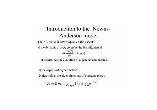
Introduction to the <strong>Newns</strong>-<br />
<strong>Anderson</strong> <strong>model</strong><br />
The NA <strong>model</strong> has two equally valid aspects<br />
a) the dynamic aspect, given by the Hamiltonian H<br />
∂ϕ(<br />
t)<br />
ih<br />
= Hϕ(<br />
t)<br />
∂t<br />
H determines the evolution of a general state in time.<br />
b) the aspects of eigenfunctions.<br />
H determines the eigen functions of constant energy<br />
E<br />
= hω<br />
ϕ ( t)<br />
= ϕ<br />
eigen 0<br />
e<br />
−iωt
creation and annihilation operators automatically take Pauli’s<br />
principle into account<br />
state<br />
1 filled with one electron,<br />
empty state<br />
creation(<br />
appearance)<br />
operator<br />
annihilation ( disappearance)<br />
a<br />
∗<br />
for<br />
one can fill state a only with one electron:<br />
state<br />
a<br />
0<br />
operator a for state a<br />
a<br />
∗<br />
∗<br />
0 = 1 a 1 =<br />
0<br />
one can take only one electron out of a state a : a 1 = 0 a 0 = 0<br />
With these definition it is easy to derive:<br />
∗<br />
∗<br />
a a 1 = 1 and a a 0 = 0 = 0×<br />
a<br />
Therefore, the operator a*a gives the number of electrons in state<br />
a<br />
namely 0 or 1.
<strong>Newns</strong>-<strong>Anderson</strong>-<strong>model</strong>,<br />
dynamics, with condition<br />
V ak < filled metal bandwidth<br />
single electron energy ε<br />
adsorbate is „reduced“ to the<br />
lowest unoccupied orbital<br />
(LUMO) |a><br />
Fermi<br />
energy<br />
E CT<br />
k final<br />
k initial<br />
metal with<br />
electron states k<br />
„dynamical charge transfer“<br />
Note, that Heisenberg‘s<br />
uncertainty principle allows<br />
residence in |a> for times<br />
shorter than ħ/E CT .<br />
V ak<br />
grows, the nearer the adsorbate<br />
comes to the surface<br />
z<br />
H = ε a † a + ∑ε<br />
a † a + ∑( V a † a + V * a † a)<br />
NA a k k k ak k ak k<br />
k<br />
k<br />
energy of<br />
LUMO<br />
number of<br />
electrons in<br />
|a><br />
energy of<br />
state k<br />
number<br />
of<br />
electrons<br />
in k<br />
Without energy for the excitation of<br />
an electron-hole pair: k final= k initial
<strong>Newns</strong>-<strong>Anderson</strong> <strong>model</strong>, adsorbate induced density of states<br />
H = ε a † a + ∑ε<br />
a † a + ∑( V a † a + V * a † a)<br />
NA a k k k ak k ak k<br />
k<br />
k<br />
For weak coupling (V ak < metallic bandwidth) H NA yields eigenfunctions | i >of the total system<br />
adsorbate and metal with a continuum of energies ε i .<br />
„adsorbate induced density of states“ ρ a<br />
(ε)dε=Σ i<br />
|| 2 δ(ε-ε i<br />
)dε<br />
is the projection of the LUMO of the combined system.<br />
Result:<br />
ε i<br />
ρ a<br />
(ε) = (1/π) (∆(ε)/(ε-ε a<br />
-Λ(ε)) 2 +∆(ε) 2<br />
This is a Lorentzian with center ε a<br />
+Λ(ε),<br />
2∆<br />
ε a<br />
+Λ(ε)<br />
with shift Λ(ε)=(1/π) P∫(∆(ε‘)dε‘)/(ε-ε‘)<br />
Fermi energy ε F<br />
and halfwidth ∆(ε) = π∫⏐V ak<br />
⏐ 2 δ(ε-ε k<br />
)dk<br />
The usual approximation is<br />
ρ<br />
a<br />
( ε ) =<br />
1<br />
π<br />
∆<br />
( ε ε )<br />
a<br />
2<br />
− +<br />
∆<br />
2<br />
0<br />
ρ a<br />
(ε)<br />
time average of electrons in |a>
Why is it possible that k final ≠ k initial (under condition of energy input)?<br />
|a><br />
Fermi<br />
energy<br />
E CT<br />
k final<br />
k initial<br />
electron after<br />
}<br />
hole dynamic CT<br />
† † † * †<br />
NA a k k k ak k ak k<br />
k<br />
k<br />
number of<br />
energy of electrons in energy of<br />
LUMO<br />
state k<br />
|a><br />
H = ε a a + ∑ ε a a + ∑ ( V a a + V a a )<br />
transformation without loss of generality<br />
z<br />
k<br />
∑<br />
initial<br />
∑<br />
V a a + V a a<br />
† * †<br />
ak k ak k<br />
k<br />
initial initial final final<br />
final
Self consistent calculations by N.D. Lang, A.R .Williams, Phys. Rev.B 18 (1978) 616,<br />
Cl, Si and Li atom adsorbed on jellium (r s =2), similarity to NA-resonances<br />
above: total electron density plots<br />
edge of the positive<br />
background<br />
Li Si Cl<br />
below: total electron density-minus superposition<br />
of atomic and bare metal electron density.<br />
Is it a Li ion in front of a sharp boundary or is it a polarised Li atom? This distinction is not unambiguously possible!<br />
∞<br />
However the surface averaged dipole moment d is still a good definition:<br />
d < 0 for electronegative adsorbates (e.g. Cl), d >0 for electropositive adsorbates e.g. Li<br />
d =−∫ ezδ<br />
n( r)<br />
d r<br />
One might call the SERS <strong>model</strong> of temporary charge transfer correctly the <strong>model</strong> of temporary<br />
change of the surface dipole moment, but I will not do that!<br />
−∞