EE 511 Solutions to Problem Set 5

EE 511 Solutions to Problem Set 5
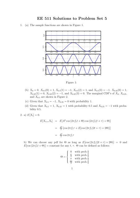
1. (a) The sample functions are shown in Figure 1.
2
X t
(0)
1
0
−1 −0.8 −0.6 −0.4 −0.2 0 0.2 0.4 0.6 0.8 1
1
t
X t
(1)
0
−1
−1 −0.8 −0.6 −0.4 −0.2 0 0.2 0.4 0.6 0.8 1
1
t
X t
(2)
0
−1
−1 −0.8 −0.6 −0.4 −0.2 0 0.2 0.4 0.6 0.8 1
1
t
X t
(3)
0
−1
−1 −0.8 −0.6 −0.4 −0.2 0 0.2 0.4 0.6 0.8 1
t
Figure 1:
(b) X 0 = 0. X 0.5 (0) = 1, X 0.5 (1) = −1, X 0.5 (2) = 1, and X 0.5 (3) = −1. X 0.25 (0) = 1,
X 0.25 (1) = 0, X 0.25 (2) = −1, and X 0.25 (3) = 0. The marginal CDF’s of X 0 , X 0.25 ,
and X 0.5 are shown in Figure 2.
(c) Given that X 0.5 = −1, X 0.25 = 0 with probability 1.
(d) Given that X 0.5 = 1, X 0.25 = 1 with probability 0.5 and X 0.25 = −1 with probability
0.5.
2. a) E[X t ] = 0.
E[X t+τ X t ] = E[A 2 cos (2πf c t + Θ) cos (2πf c (t + τ) + Θ)]
= A2
2 [cos 2πf cτ + E[cos (2πf c (2t + τ) + 2Θ)]]
= A2
2 cos 2πf cτ
b) We can choose any pdf for Θ as long as E[cos (2πf c (2t + τ) + 2Θ)] = 0 and
E[cos (2πf c t + Θ)] = constant for any t, τ. Θ can be defined as follows:
⎧
⎪⎨
Θ =
⎪⎩
0 with prob. 1 4
π
2
with prob. 1 4
π with prob. 1 4
3π
2
with prob. 1 4
1

CDf of X 0
F
X0
(x)
CDF of X 0.25
F
X0.25
(x)
CDF of X 0.25
F
X0.5
(x)
1
0.5
0
−2 −1.5 −1 −0.5 0 0.5 1 1.5 2 2.5 3
x
1
0.5
0
−2 −1.5 −1 −0.5 0 0.5 1 1.5 2 2.5 3
x
1
0.5
0
−2 −1.5 −1 −0.5 0 0.5 1 1.5 2 2.5 3
x
Figure 2:
Another possible choice for Θ is:
⎧
⎪⎨
Θ =
⎪⎩
0 with prob. 1 12
π
4
with prob. 1 6
π
2
with prob. 1 12
3π
4
with prob. 1 6
π with prob. 1 12
5π
4
with prob. 1 6
3π
2
with prob. 1 12
7π
4
with prob. 1 6
A more general choice for f Θ (θ) can be made as follows:
(i) Let us assume that the range of Θ is from 0 to 2π.
(ii) The condition for mean to be constant can be obtained as follows:
E[cos (2πf c t + Θ)] = ∫ 2π
0 cos (2πf c t + θ)f Θ (θ)dθ
= ∫ π
0 cos (2πf ct + θ)f Θ (θ)dθ + ∫ 2π
π cos (2πf ct + θ)f Θ (θ)dθ
(using θ ′ = θ − π) = ∫ π
0 cos (2πf ct + θ)f Θ (θ)dθ + ∫ π
0 cos (2πf ct + θ ′ + π)f Θ (θ ′ + π)dθ ′
= ∫ π
0 cos (2πf ct + θ)f Θ (θ)dθ + ∫ π
0 [− cos (2πf ct + θ ′ )]f Θ (θ ′ + π)dθ ′
= ∫ π
0 cos (2πf ct + θ)[f Θ (θ) − f Θ (θ + π)]dθ
Therefore, if f Θ (θ) = f Θ (θ + π) for θ in [0,π], then E[cos (2πf c t + Θ)] = 0.
2

(iii) The additional condition for the auto-correlation funtion to be a function of τ can
be obtained as follows:
E[cos (2πf c (2t + τ) + 2Θ)] = ∫ 2π
0 cos (2πf c (2t + τ) + 2θ)f Θ (θ)dθ
(using φ = 2θ) = 1 2
= 1 2
(using φ ′ = φ − 2π) = 1 2
= 1 2
+ 1 2
+ 1 2
∫ 4π
0 cos (2πf c (2t + τ) + φ)f Θ
( φ
2)
dφ
∫ 2π
0 cos (2πf c (2t + τ) + φ)f Θ
( φ
2)
dφ
∫ 4π
2π cos (2πf c(2t + τ) + φ)f Θ
( φ
2)
dφ
∫ 2π
0 cos (2πf c (2t + τ) + φ)f Θ
( φ
2)
dφ
( )
∫ 2π
0 cos (2πf c (2t + τ) + φ ′ φ
)f ′
Θ + π dφ ′
2
[
∫ ( ) )]
2π
0 cos (2πf c (2t + τ) + φ) f φ
Θ 2 +
(φ ′
fΘ + π dφ.
2
Assuming that we satisfy the condition from (ii) above, we get
E[cos (2πf c (2t + τ) + 2Θ)] =
Now, proceeding as in (ii), we need
)
f Θ
( φ
2
∫ 2π
0
cos (2πf c (2t + τ) + φ)f Θ
( φ
2
( ) φ + π
= f Θ
2
for φ/2 in [0,π]. Equivalently, we need
(
f Θ (θ) = f Θ θ + π )
2
)
dφ.
for θ in [0,π/2].
(iv) Combining the conditions from (ii) and (iii), we get
(
f Θ (θ) = f Θ θ + kπ )
2
(1)
for θ in [0,π/2] and k = 1, 2, 3. Therefore, we can choose any arbitrary f Θ (θ) for
θ in [0,π/2] such that
∫ π
2
f Θ (θ)dθ = 1 4 .
f Θ (θ) for θ in [π/2, 2π] can be set using (1).
A sample pdf that fives a W.S.S. X t is shown in Figure 3.
0
3

f (θ)
Θ
2/3π
1/3π
0 π/4 π/2 3π/4 π 5π/4 3π/2 7π/4 2π
θ
Figure 3:
3. a) E[Y t ] = E[X t cos (2πf c t + Θ)]. Since Θ and X t are independent, E[Y t ] = E[X t ]E[cos (2πf c t + Θ)
m X E[cos (2πf c t + Θ)] = 0.
Y t is W.S.S..
R Y (t + τ,t) = E[X t X t+τ ]E[cos (2πf c t + Θ) cos (2πf c (t + τ) + Θ)]
= 1 2 R X(τ)[cos 2πf c τ + E[cos 2πf c (2t + τ) + 2Θ]]
= 1 2 R X(τ) cos 2πf c τ.
b) E[Y t ] = E[X t ] cos 2πf c t = m X cos 2πf c t is a function of time. Y t is not W.S.S.
4. E[X t ] = E[X 1 ] cos 2πf c t + E[X 2 ] sin 2πf c t. For the mean to be independent of t, we
need
E[X 1 ] = E[X 2 ] = 0.
R X (t,t + τ) = E[(X 1 cos 2πf c (t + τ) + X 2 sin 2πf c (t + τ))(X 1 cos 2πf c t + X 2 sin 2πf c t)]
=
( E[X
2
1 ] + E[X2]
2 )
cos 2πf c τ
2
+ 2E[X 1 X 2 ] sin 2πf c (2t + τ)
+
( E[X
2
1 ] − E[X2]
2 )
cos 2πf c (2t + τ).
2
For R X (t,t + τ) to be independent of t, we need
E[X 1 X 2 ] = 0 and E[X 2 1] = E[X 2 2].
The conditions derived above are both necessary and sufficient.
4

5.
E [|X t+τ − X t | 2 ] = E [ X t+τ X ∗ t+τ]
− E [Xt+τ X ∗ t ] − E [ X t X ∗ t+τ]
+ E [Xt X ∗ t ]
(Since X t is W. S. S.) = R X (0) − R X (τ) − R ∗ X(τ) + R X (0)
= 2R X (0) − 2Re(R X (τ))
(Since R X (0) is real)
= 2Re(R X (0) − R X (τ)).
6. (a)
Adding the above equations, we get
X 0 = 0
ρ n−1 (X 1 = W 1 )
ρ n−2 (X 2 = ρX 1 + W 2 )
. .
ρ 0 (X n = ρX n−1 + W n ).
X n = W n + ρW n−1 + · · · + ρ n−1 W 1 .
Therefore, E[X n ] = 0 and V ar(X n ) = 1 + ρ 2 + · · · + ρ 2n−2 .
(b) E[X n X n+k ] = E[X n (ρX n+k−1 + W n+k )] = ρE[X n X n+k−1 ]. Therefore, we have
E[X n X n+k ] = ρ k E[X 2 n] = ρ k (1 + ρ 2 + · · · + ρ 2n−2 ).
(c) No. E[X n X n+k ] is dependent on n.
7. Using Cauchy-Schwartz inequality and (geometric mean ≤ arithmetic mean), we have
√
|R XY (τ)| ≤ R X (0)R Y (0) ≤ 0.5[R X (0) + R Y (0)].
8. R X (t+τ,t) = E[X t+τ X t ] = E[Y t+τ Z t+τ Y t Z t ]. Since Y t and Z t are independent random
processes, R X (t + τ,t) = E[Y t+τ Y t ]E[Z t+τ Z t ] = R Y (τ)R Z (τ). X t is also W.S.S..
9. a) The transfer function of the filter (whose input is X t and output is Y t ) is
H(f) = 1 − e −j2πfT = 1 − cos 2πfT + j sin 2πfT.
S Y (f) = S X (f)|H(f)| 2
= S X (f) [(1 − cos 2πfT) 2 + (sin 2πfT) 2 ]
= 2S X (f)[1 − cos 2πfT)] = 4S X (f)(sinπfT) 2
b) If f ≪ 1/T such that πfT is very small, then sinπfT is approximately equal to
πfT. Therefore, S Y (f) = 4π 2 f 2 T 2 S X (f). A scaled version of the same power spectral
density would be obtained if Y t is obtained from X t using a differentiator, i.e., we will
get S Y (f) = 4π 2 f 2 S X (f).
5

10. a) E[Z t ] = E[X t ] + E[Y t ] = m X + m Y .
Z t is W.S.S..
R Z (t,s) = E[(X t + Y t )(X s + Y s )]
= R X (t,s) + R XY (t,s) + R Y X (t,s) + R Y (t,s)
(using τ = t − s) = R X (τ) + R XY (τ) + R Y X (τ) + R Y (τ)
b) S Z (f) = S X (f) + S XY (f) + S Y X (f) + S Y (f).
c) If X t and Y t are uncorrelated and zero-mean, then S Z (f) = S X (f) + S Y (f). If they
are non-zero mean random processes and uncorrelated, then S Z (f) = S X (f)+S Y (f)+
2m X m Y δ(f).
11. (a) R S (t,s) = E[S t S s ] = E[(X t + Y t )(X s + Y s )] = R X (t,s) + R XY (t,s) + R Y X (t,s) +
R Y (t,s). Since, X t and Y t are jointly W. S. S., we have
Similarly, we can show
R S (τ) = R X (τ) + R XY (τ) + R XY (−τ) + R Y (τ).
R D (τ) = R X (τ) − R XY (τ) − R XY (−τ) + R Y (τ).
12.
(b) R XS (t,s) = E[X t (X s +Y s )] = R X (t,s)+R XY (t,s). Therefore, we have R XS (τ) =
R X (τ) + R XY (τ).
(c) R SD (t,s) = E[(X t + Y t )(X s − Y s )] = R X (t,s) − R XY (t,s) + R Y X (t,s) − R Y (t,s).
Therefore, we have R SD (τ) = R X (τ) − R XY (τ) + R XY (−τ) − R Y (τ).
R ZW (t,s) = E[Z t W s ]
[∫ ∞
∫ ∞
]
= E h 1 (τ 1 )X t−τ1 dτ 1 h 2 (τ 2 )Y s−τ2 dτ 2
−∞
−∞
=
=
=
∫ ∞
−∞
∫ ∞
−∞
∫ ∞
−∞
∫ ∞
−∞
∫ ∞
−∞
h 1 (τ 1 )h 2 (τ 2 )E[X t−τ1 Y s−τ2 ]dτ 1 dτ 2
h 1 (τ 1 )h 2 (τ 2 )R XY (t − s − τ 1 + τ 2 )dτ 1 dτ 2
[∫ ∞
h 1 (τ 1 ) h 2 (τ 2 )R XY (t − s − τ 1 + τ 2 )dτ 2
]dτ 1
−∞
From the above result, we see that R ZW (t,s) is a function of τ = t − s and is the
convolution of R XY (τ), h 1 (τ) and h 2 (−τ). Therefore, we have
S ZW (f) = S XY (f)H 1 (f)H ∗ 2(f).
6

13. (a) Y n = X n + X n−1 + X n−2 .
∞∑ e −λ λ k
φ Xn (s) = E[e sXn ] = e sk = e −λ ∑ ∞
k=0
k!
k=0
λe s
k!
= e −λ e λes = e −λ(1−es) .
Since X n , X n−1 , and X n−2 are independent and identically distributed, we have
φ Yn (s) = E[e sYn ] = E[e sXn ]E[e sX n−1
]E[e sX n−2
] = E[e sXn ] 3 = e −3λ(1−es) .
Therefore, Y n is a Poisson random variable with parameter 3λ, i. e.,
P[Y n = k] = e −3λ(3λ)k
k!
∀k ≥ 0.
(b)
φ Yn (s) = E[e sYn ] = E[e sXn ]E[e sX n−1
]E[e sX n−2
] = e −(λn+λ n−1+λ n−2 )(1−e s) .
Therefore, Y n is a Poisson random variable with parameter λ n + λ n−1 + λ n−2 , i.
e.,
P[Y n = k] = e −(λn+λ n−1+λ n−2 ) (λ n + λ n−1 + λ n−2 ) k
∀k ≥ 0.
k!
7