Cellular Systems Cellular Concepts The cellular concept was a ...

EE5401 Cellular Mobile Communications 


Cellular Systems 

Cellular Concepts 

 

 

The cellular concept was a major breakthrough in 

solving the problem of spectral congestion and user 

capacity. It offered very high capacity in a limited 

spectrum allocation without any major technological 

changes. 

The cellular concept has the following system level 

ideas 

• Replacing a single, high power transmitter with many 

low power transmitters, each providing coverage to 

only a small area. 

• Neighbouring cells are assigned different groups of 

channels in order to minimise interference. 

 

 

Reuse can be done once the total interference from all 

users in the cells using the same frequency (cochannel 

cell) for transmission suffers from sufficient 

attenuation. Factors need to be considered include: 

• Geographical separation (path loss) 

• Shadowing effect 

The actual radio coverage of a cell is known as the 

cell footprint. 

• Irregular cell structure and irregular placing of the 

transmitter may be acceptable in the initial system 

design. However as traffic grows, where new cells and 

channels need to be added, it may lead to inability to 

reuse frequencies because of co-channel interference. 

• For systematic cell planning, a regular shape is 

assumed for the footprint. 

 

• The same set of channels is then reused at different 

geographical locations. 

When designing a cellular mobile communication 

system, it is important to provide good coverage and 

services in a high user-density area. 

• Coverage contour should be circular. However it is 

impractical because it provides ambiguous areas with 

either multiple or no coverage. 

• Due to economic reasons, the hexagon has been chosen 

due to its maximum area coverage. 

Institute for Infocomm Research 43 National University of Singapore 

Institute for Infocomm Research 44 National University of Singapore



R 

R 

R 

2 

2 

2 

Atri = 1.3R 

Asq 

= 2.0R 

Ahex 

= 2.6R 

• Interference tier : A set of co-channel cells at the same 

distance from the reference cell is called an 

interference tier. The set of closest co-channel cells is 

call the first tier. There is always 6 co-channel cells in 

the first tier. 

• Hence, a conventional cellular layout is often defined 

by a uniform grid of regular hexagons. 

Frequency reuse : 

• A cellular system which has a total of S duplex 

channels. 

• S channels are divided among N cells, with each cell 

uses unique and disjoint channels. 

• If each cell is allocated a group of k channels, then 

S = kN . 

 

Co-ordinates for hexagonal cellular geometry 

• With these co-ordinates, an array of cells can be laid 

out so that the center of every cell falls on a point 

specified by a pair of integer co-ordinates. 

 

Terminology 

• Cluster size : The N cells which collectively use the 

complete set of available frequency is called the 

cluster size. 

• Co-channel cell : The set of cells using the same set of 

frequencies as the target cell. 

If ( ∆ u , ∆v) 

= ( i, 

j) 

, i,j are known as the shift 

parameters, then the distance between the two cell 

centres is given by 

2 

2 

D = i + j + ij ⋅ 3R 

(Cosine’s Rule) 





 

Designing a cellular system 

Examples: N=3,4,7,9,12,13 

Proof : to obtain the area of the cluster and compare 

with the area of a single cell. 

 

The cluster size must satisfy 

2 2 

N = i + ij + j where i, j str non-negative integers. 

 

Can also verify that 

D 

Q = = 3N 

where Q is the co-channel reuse ratio. 

R 





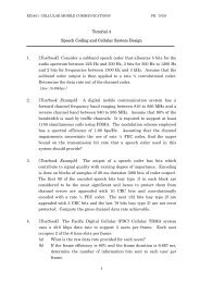
Handover / Handoff 

 

Occurs as a mobile moves into a different cell during 

an existing call, or when going from one cellular 

system into another. 

• It must be user transparent, successful and not too 

frequent. 

• If the slope of the short-term average received signal 

is steep, handover should carry out fast. Information 

about vehicle speed is important. 

Handover take place 

f1 

f2 

P HO 

• Not only involves identifying a new BS, but also 

requires that the voice and control signals be allocated 

to channels associated with the new BS. 

Time taken to 

complete handover 

P min 

 

Once a particular signal level P min is specified as the 

minimum usable signal for acceptable voice quality 

at the BS receiver, a slightly stronger signal level 

P HO is used as a threshold at which a handover is 

made. 

P HO 

= P min 

+ ∆ 

• If ∆ is too large ⇒ unnecessary handovers 

• If ∆ is too small ⇒ insufficient time to complete 

handovers, call may drop due to poor received signal 

quality. 

• Running average should be used to avoid unwanted 

handover due to momentary fading. 

 

Dwell Time 

• The time over which a user remains within one cell is 

called the dwell time. 

• The statistics of the dwell time are important for the 

practical design of handover algorithms. 

• The statistics of the dwell time vary greatly, 

depending on the speed of the user and the type of 

radio coverage. 





 

 

Handover indicator 

• Each BS constantly monitors the signal strengths of 

all of its reverse voice channels to determine the 

relative location of each mobile user with respect to 

the BS. This information is forwarded to the MSC 

who makes decisions regarding handover. 

• Mobile assisted handover (MAHO) : The mobile 

station measures the received power from 

surrounding BSs and continually reports the results of 

these measurements to the serving BS. 

Prioritizing Handover 

• Dropped call is considered a more serious event than 

call blocking. Channel assignment schemes therefore 

must give priority to handover requests. 

 

which a handover is usually required leaves room for 

queueing handover request. 

Practical handover 

• High speed users and low speed users have vastly 

different dwell times which might cause a high 

number of handover requests for high speed users. 

This will result in interference and traffic 

management problem. 

• The Umbrella Cell approach will help to solve this 

problems. High speed users are serviced by large 

(macro) cells, while low speed users are handled by 

small (micro) cells. 

• A fraction of the total available channels in a cell is 

reserved only for handover requests. However, this 

reduces the total carried traffic. Dynamic allocation 

can improve this. 

• Queuing of handover requests is another method to 

decrease the probability of forced termination of a call 

due to a lack of available channel. The time span over 





 

 

A hard handover does “break before make”, ie. The 

old channel connection is broken before the new 

allocated channel connection is setup. This obviously 

can cause call dropping. 

In soft handover, we do “make before break”, ie. The 

new channel connection is established before the old 

channel connection is released. This is realized in 

CDMA where also BS diversity is used to improve 

boundary condition. 

A 

Hard: 

B 

Interference and System Capacity 

 

 

In a given coverage area, there are several cells that 

use the same set of frequencies. These cells are called 

co-channel cells. The interference between signals 

from these cells is called co-channel interference. 

If all cells are approximately of the same size and the 

path loss exponent is the same throughout the coverage 

area, the transmit power of each BS is almost equal. 

We can show that worse case signal to co-channel 

interference is independent of the transmitted power. 

It becomes a function of the cell radius R, and the 

distance to the nearest co-channel cell D’. 

A 

Soft: 

B 

(a) Received power at a distance d from the 

transmitting antenna is approximated by 

−n 

⎛ d ⎞ 

Pr 

( d) 

= P0 

⎜ 

d 

⎟ or 

⎝ 0 ⎠ 

⎛ d ⎞ 

P r ( d) 

( dBm ) = P0 ( dBm ) −10nlog 

⎜ 

⎟ 

⎝ d0 

⎠ 

(b) Useful signal at the cell boundary is the 

weakest, given by P r (R). Interference signal from 

the co-channel cell is given to be P r (D′) 

. 





(c) D’ is normally approximated by the base station 

separation between the two cells D, unless when 

accuracy is needed. Hence 

−n 

R 

SIR = 

−n 

D 

• If only first tier co-channel cells are considered, then 

i 0 = 6. 

• Unless otherwise stated, normally assuming 

for all i. 

D i ≈ D 

 

Outage probability : the probability that a mobile 

station does not receive a usable signal. 

• For GSM, this is 12 dB and for AMPS, this is 18 dB. 

If there is 6 co-channel cells, then 

n 

( D R) ( 3N 

) 

SIR = = 

6 

6 

Exercise : please verify this 

• For n=4, a minimum cluster size of N=7 is needed to 

meet the SIR requirements for AMPS. 

n 

 

For the forward link, a very general case, 

−n 

R 

SIR = 

i0 

−n 

∑ Di 

i= 

1 

where D i is the distance of the ith interfering cell 

from the mobile, i 0 is the total number of co-channel 

cells exist. 

• For n=4, a minimum cluster size of N=4 is required to 

meet the SIR requirements for GSM 





- More accurate SIR can be obtained by computing 

the actual distance. 

- Aproximation in distance has been made on the 

2 nd tier onwards. 

- Our computation of outage only based on path loss. 

For more accurate modeling, shadowing and fast 

fading need to be taken into consideration. This will 

not be covered in this course. 





Coverage Problems 

 

Revision: 

- Recall that the mean measured value, 

⎛ d ⎞ 

PL( 

d) 

dB = PL( 

d0) 

dB + 10n 

log 

⎜ 

⎟ or 

⎝ d0 

⎠ 

P r ( d) 

dB = PtdB 

− PL( 

d) 

dB 

[ P ( γ ] 

β ( γ ) = P r R) 

> - cell boundary coverage, 

β ( γ ) 

∞ 

= ∫ 

γ 

1 

2πσ 

X dB 

⎛ ⎞ 

⎜γ 

− P 

= r ( R) 

Q ⎟ 

⎜ ⎟ 

⎝ 

σ X dB ⎠ 

⎡ 

2⎤ 

⎢ 1 ⎛ 

⎞ 

⎜ X − 

− dB Pr 

( R) 

exp 

⎟ ⎥dX 

⎢ ⎜ 

⎟ ⎥ dB 

2 

⎢⎣ 

⎝ 

σ X dB ⎠ ⎥⎦ 

where Q(x) is the standard normal distribution. 

• must know how to use the table. 

 

- Measurement shows that at any value of d, the 

path loss PL (d) 

at a particular location is random 

and distributed log-normally (normal in dB) about 

this mean value. 

Pr ( d) 

dB = Pr 

( d) 

dB + X σ 

where X σ is a zero-mean Gaussian distributed 

random variable (in dB) with standard deviation σ 

(in dB). 

Boundary coverage 

 

Cell coverage 

• Proportion of locations within the area defined by the 

cell radius R, receiving a signal above the threshold γ. 

1 

U ( γ ) = ∫ P[ Pr 

( r) 

> γ ] dA 

A 

A 

1 

R 2π 

⎛ P r ⎞ 

Q⎜γ 

− r ( ) 

= ∫ ∫ 

⎟ ⋅ rdr ⋅ dθ 

2 

πR 

⎜ 

X 

⎟ 

0 0 ⎝ 

σ 

dB ⎠ 

2 

R ⎛ P r ⎞ 

Q⎜γ 

− 

= 

r ( ) 

∫ 

⎟ ⋅ rdr 

R ⎜ 

X 

⎟ 

0 ⎝ 

σ 

dB ⎠ 

• Therefore, there will be a proportion of locations at 

distance R (cell radius) where a terminal would 

experience a received signal above a threshold γ. (γ is 

usually the receiver sensitivity) 

The solution is given in the Rappaport p.107 (1 st 

edition). 





Solution can be found using the graph provided. (n : 

path loss exponent) 

 

The mean signal level at any distance is determined 

by path loss and the variance is determined by the 

resulting fading distribution (log-normal shadowing, 

Rayleigh fading, Nakagami-m, etc). In this course, we 

will deal with log-normal shadowing only. 

 

The proportion of locations covered at a given 

distance (cell boundary, for example) from BS can be 

found directly from the resultant signal pdf/cdf. 

 

The proportion of locations covered within a circular 

region defined by a radius R (the cell area, for 

example) can be found by integrating the resultant 

cdf over the cell area. 

Example: if n=4, σ=8 dB, and if the boundary is to 

have 75% coverage (75% of the time the signal is to 

exceed the threshold at the boundary), then the 

area coverage is equal to 94%. 

If n=2, σ=8 dB, and if the boundary is to have 75% 

coverage, then the area coverage is equal to 91%. 

 

An operator needs to meet certain coverage criteria. 

This is typically the “90% rule” – 90% of a given 

geographical area must be covered for 90% of the 

time. 





Cellular Traffic 

- Call holding time (H) : the average duration of a call. 

- Request rate (λ) : average number of call requests per 

unit time. 

 

The basic consideration in the design of a cellular 

system is the sizing of the system. Sizing has two 

components to be considered. 

- Coverage area 

- Traffic handling capability 

• After the system is sized, channels are assigned to 

cells using the assignment schemes mentioned before. 

 

Traffic flow or intensity A 

• Measured in Erlang, which is defined as the callminute 

per minute. 

• Total offered traffic for such a system is given as 

A = λ ⋅ H 

Exercise : There are 3000 calls per hour in a cell, 

each lasting an average of 1.76 min. 

 

Terminology in traffic theory 

Offered traffic A = (3000/60)(1.76) = 88 Erlangs 

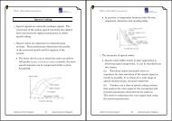
- Trunking : exploits the statistical characteristics of 

the users calling behaviour. Any efficient 

communication system relies on trunking to 

accommodate a large number of users with a limited 

number of channels. 

- Grade of service (GoS) : A user is allocated a channel 

on a per call basis. GoS is a measure of the ability of 

a user to access a trunked system during the busiest 

hour. It is typically given as the likelihood that a call 

is blocked (also known as blocking probability 

mentioned before). 

- Trunking theory : is used to determine the number of 

channels required to service a certain offered traffic 

at a specific GoS. 

 

 

 

If the offered traffic exceeds the maximum possible 

carried traffic, blocking occurs. There are three 

different strategies to be used. 

- Blocked calls cleared 

- Blocked calls delayed 

Trunking efficiency : is defined as the carried traffic 

intensity in Erlangs per channel, which is a value 

between zero and one. It is a function of the number 

of channels per cell and the specific GoS parameters. 

Call arrival process: it is widely accepted that calls 

have a Poisson arrival. 





Over an observation period T, divide this time into 

n sub-intervals. 

- only one arrival can occur in any one sub-interval. 

- call arrivals are independent from each other. 

- the probability that an arrival occurs in one of 

the sub-intervals is proportional to the subinterval 

length. 

The probability of exactly k arrivals in n subintervals 

can be evaluated using the binomial 

distribution. In the limit when n→∞ , this 

approach to a Poisson Process, with its mean equal 

to λ T . 

(Refer to tutorial 1 and extend the concept from 

Poisson distribution to Poisson Process) 

( λT 

) 

k 

pk 

= exp 

k! 

( − λT 

) 

- The probability that a call terminates within one 

subinterval is proportional to its length. 

- The call termination occurs independently of which 

subinterval is considered. 

The probability that the holding time h is less than 

or equal t is given as 

n 

⎛ µ t ⎞ 

1 − Fh ( t) 

= 1 − P( 

h ≤ t) 

= P( 

h > t) 

= lim ⎜1 

− ⎟ = exp µ 

n→∞⎝ 

n ⎠ 

∴Fh ( t) 

= 1− 

exp( − µ t) ⇒ fh( 

t) 

= µ exp( − µ t) 

This gives a mean holding time of H =1 µ . 

( − t) 

Markov chain : probability that the next state is x n+ 1 

depends only upon the current state x n and not any 

previous value. A special case is the birth-death 

process. 

 

Mean inter-arrival time 

( τ ≤ t) = 1− 

P( τ > t) = 1− 

P( no ) = 1− 

( − λt) 

λ exp( − λt) 

Fτ 

( t) 

= P 

arrival exp 

∴ fτ 

( t) 

= 

 

Block calls cleared : Assuming that there are altogether 

C trunks, and 

• An infinite subscriber population 

 

Memoryless property of the negative exponential 

distribution : the past history of an exponentially 

distributed random variable has no influence in 

predicting its future. 

• Poisson call arrivals with rate λ calls/sec 

• Exponentially distributed call durations with mean 

H =1/ µ . 

 

Call holding time : it is normally assume that it has a 

negative exponential distribution. 

• Blocked calls are cleared. 





Under steady state conditions 

Pn = n ⋅ P n 

λδ ⋅ − 1 µδ 

Solving for different values of n, we have 

n 

λ 

λ 1 ⎛ λ ⎞ 

P 1 = P 0 , …, Pn 

= Pn 

−1 

= ⎜ ⎟ P0 

, … 

µ 

nµ 

n! 

⎝ µ ⎠ 

C 

From ∑ P n = 1, we get 

n= 

0 

1 

P0 

= 

C n 

1 ⎛ λ ⎞ 

∑ ⎜ ⎟ 

n= 

0 n! 

⎝ µ ⎠ 

The probability of blocking for C trunked channel is 

C 

1 ⎛ λ ⎞ 

⎜ ⎟ 1 

C 

C 

A 

1 ⎛ λ ⎞ C! 

⎟ = 

⎝ µ 

GoS = P = ⎜ 

⎠ 

c P 

= C! 

0 

C! 

C 

⎝ µ ⎠ C n 

1 ⎛ λ ⎞ 1 n 

∑ ⎜ ⎟ ∑ A 

n= 

n ⎝ ⎠ n= 

0 n! 

0 ! µ 

which is the Erlang B formula, and A = λ H = λ µ . 

• Must know how to use the table. 

Examples on Erlang B models 

 

1. There are 3000 calls per hour in a cell, each lasting 

an average of 1.76 minutes. For a 2% blocking 

probability, how many channels are needed in the 

cell? 

2. A cell contains 50 channels. The average call 

duration is 100s. How many calls per hour can be 

handle if PB=2%? 

Blocked calls delayed : in this model, the blocked 

calls are allowed to queue up and wait to be served. 

Normally assume that the queue is infinitely long 

(M/M/C/∞) 

At steady state, 

λδ ⋅ Pn − 1 = nµδ 

⋅ P n for k ≤ C 

λδ ⋅ Pn − 1 = Cµδ 

⋅ P n for k ≥ C 

This leads to 

⎧ 

n 

1 ⎛ λ ⎞ 

⎪ ⎜ ⎟ P0 

n ≤ C 

n! 

⎝ µ 

P = ⎠ 

n ⎨ n 

⎪ 1 ⎛ λ ⎞ 1 

≥ 

⎪ 

⎜ ⎟ P n C 

− 

⎩C! 

n C 0 

⎝ µ ⎠ C 

From = 1 

n∑ ∞ P n , we get 

= 0 





P 

0 

= 

C 

∑ − 1 

n= 

0 

1 ⎛ λ ⎞ 

⎜ ⎟ 

n! 

⎝ µ ⎠ 

n 

1 

1 ⎛ λ ⎞ 

+ ⎜ ⎟ 

C! 

⎝ µ ⎠ 

C 

1 

⎛ λ ⎞ 

⎜1 

− ⎟ 

⎝ µ C ⎠ 

The probability that the call will not have 

immediate access to a channel (i.e. having nonzero 

delay) 

Pr( delay 

> 0) = ∑ ∞ P 

= 

k 

k C 

C 

A 1 

= P 

C! 

A 

1− 

C 

where A = λ / µ . This is the Erlang C formula. 

- This probability of non-zero delay that can be 

tolerated is also known to be the GoS parameter of 

the Erlang C system. 

- If no channels are immediately available, the call 

is delayed, and the probability that the delayed 

call is forced to wait more than t seconds is given 

by the probability that a call is delayed, multiplied 

by the conditional probability that the delay is 

greater than t seconds (the delay threshold). 

Pr(delay > t) 

= Pr(delay > 0) Pr(delay > t delay > 0) 

= Pr(delay > 0) exp[ −( 

C − A) 

t / H ] 

- The average delay D for all calls in a queued 

system is given by 

∞ 

H 

D = ∫ Pr(delay > t) 

dt = Pr(delay > 0) 

0 

C − A 

or the average delay for those calls which are 

queue is given by H /( C − A) 

. 

0 

Note: Proof for 

Pr( delay > t delay > 0) = exp[ −( 

C − A) 

t / H ] 

Consider C=1, this corresponding to the M/M/1 queue 

model. The waiting time W consists of the service times of 

the existing N customers in the system, ie., 

W = S1 + S2 

+ L+ 

S N where S i follows exponential 

distribution fS ( t) 

= µ exp( − µ t) 

and W is the sum of these N 

i 

independent random variables. Note that implicity we 

assume that N > 0 . 

λ λ n 

Also can easily show that P n = (1 − )( ) , i.e. n follows a 

µ µ 

geometric distribution (memoryless property). 

The pdf of W is then given by 

Erlang( 

n+ 

1, µ ) 

64748 4 

∞ 

∞ n 

( µ t) 

−µ 

t λ λ n 

fW 

( t) 

= ∑ f 

W | n 

( t, 

n) 

Pn 

= ∑ µ e ⋅ (1 − )( ) 

n= 

0 

n= 

0 n! 

µ µ 

−( 

µ −λ) 

t 

= ( µ − λ) 

e 

Note that µ = 1/ H , A = λH 

, integrate this from t to ∞ will 

obtain Pr( delay > t delay > 0) 

For M/M/C queue, the system behaves as an M/M/1 queue 

with higher service rate C µ (rather than µ ). 





Channel Assignment Strategies 

 

Channel allocation schemes can affect the performance 

of the system. 

Fixed Channel Allocation (FCA) : 

• Channels are divided in sets. 

• A set of channels is permanently allocated to each cell 

in the network. Same set of channels must be 

assigned to cells separated by a certain distance to 

reduce co-channel interference. 

• Any call attempt within the cell can only be served by 

the unused channels in that particular cell. The 

service is blocked if all channels have used up. 

• Most easiest to implement but least flexibility. 

• An modification to this is ‘borrowing scheme’. Cell 

(acceptor cell) that has used all its nominal channels 

can borrow free channels from its neighboring cell 

(donor cell) to accommodate new calls. 

• Borrowing can be done in a few ways: borrowing from 

the adjacent cell which has largest number of free 

channels, select the first free channel found, etc. 


• To be available for borrowing, the channel must not 

interfere with existing calls. The borrowed channel 

should be returned once the channel becomes free. 

Dynamic Channel Allocaton (DCA) : 

• Voice channels are not allocated to any cell 

permanently. All channels are kept in a central pool 

and are assigned dynamically to new calls as they 

arrive in the system. 

• Each time a call request is made, the serving BS 

requests a channel from the MSC. It then allocates a 

channel to the requested cell following an algorithm 

that takes into acount the likelihood of future blocking 

within the cell, the reuse distance of the channel and 

other cost functions ⇒ increase in complexity 

• Centralized DCA scheme involves a single controller 

selecting a channel for each cell. Distributed DCA 

scheme involves a number of controllers scattered 

across the network. 

• For a new call, a free channel from central pool is 

selected based on either the co-channel distance, 

signal strength or signal to noise interference ratio. 

Flexible channel assignment 




 

• Divide the total number of channels into two groups, 

one of which is used for fixed allocation to the cells, 

while the other is kept as a central poor to be shared 

by all users. 

• Mix the advantages the FCA and DCA, available 

schemes are scheduled and predictive. 

Channels need to be assigned to users to accommodate 

- new calls 

- handovers 

With the objective of increasing capacity and 

minimizing probability of a blocked call. 

 

System Expansion Techniques 

As demand for wireless services increases, the number 

of channels assigned to a cell eventually becomes 

insufficient to support the required number of users. 

More channels must therefore be made available per 

unit area. 

• This can be accomplished by dividing each initial cell 

area into a number of smaller cells, a technique 

known as cell-splitting. 

• It can also be accomplished by having more channels 

per cell, i.e. by having a smaller reuse factor. 

However, to have a smaller reuse factor, the cochannel 

interference must be reduced. This can be 

done by using antenna sectorization. 

 

Cell splitting 

• Cell splitting increases the number of BSs in order to 

increase capacity. There will be a corresponding 

reduction in antenna height and transmitter power. 

• Cell splitting accommodates a modular growth 

capability. This in turn leads to capacity increase 





essentially via a system re-scaling of the cellular 

geometry without any changes in frequency planning. 

• Small cells lead to more cells/area which in turn leads 

to increased traffic capacity. 

• For new cells to be smaller in size, the transmit power 

must be reduced. If n=4, then with a reduction of cell 

radius by a factor of 2, the transmit power should be 

reduced by a factor of 2 4 (why?) 

• In theory, cell splitting could be repeated indefinitely. 

In practice it is limited 

1. by the cost of base stations 

2. handover (fast and low speed traffic) 

3. not all cells are split at the same time : practical 

problems of BS sites, such as co-channel 

interference exist 

 

4. Innovative channel assignment schemes must 

be developed to address this problem for 

practical systems. 

Sectorization 

• Keep the cell radius but decrease the D/R ratio. In 

order to do this, we must reduce the relative 

interference without increasing the transmit power. 

• Sectorization relies on antenna placement and 

directivity to reduce co-channel interference. Beams 

are kept within either a 60° or a 120° sector. 





• If we partition a cell into three 120° sectors, the 

number of co-channel cells are reduced from 6 to 2 in 

the first tier. 

• Using six sectors of 60°, we have only one co-channel 

cell in the first tier. 

• Each sector is limited to only using 1/3 or 1/6 of the 

available channels. We therefore have a decrease in 

trunking efficiency and an increase in the number of 

required antennas. 

• But how can the increase in system capacity be 

achieved? 





 

Micro cells 

• Micro cells can be introduced to alleviate capacity 

problems caused by “hotspots”. 

• By clever channel assignment, the reuse factor is 

unchanged. As for cell splitting, there will occur 

interference problems when macro and micro cells 

must co-exist.

Cellular Systems Cellular Concepts The cellular concept was a ...

You also want an ePaper? Increase the reach of your titles

Delete template?

Save as template?