Neural-Network-Based State Feedback Control of a ... - IEEE Xplore
Neural-Network-Based State Feedback Control of a ... - IEEE Xplore
Neural-Network-Based State Feedback Control of a ... - IEEE Xplore

You also want an ePaper? Increase the reach of your titles
YUMPU automatically turns print PDFs into web optimized ePapers that Google loves.
<strong>IEEE</strong> TRANSACTIONS ON NEURAL NETWORKS, VOL. 19, NO. 12, DECEMBER 2008 2073<br />
<strong>Neural</strong>-<strong>Network</strong>-<strong>Based</strong> <strong>State</strong> <strong>Feedback</strong> <strong>Control</strong> <strong>of</strong><br />
a Nonlinear Discrete-Time System<br />
in Nonstrict <strong>Feedback</strong> Form<br />
Sarangapani Jagannathan, Senior Member, <strong>IEEE</strong>, and Pingan He<br />
Abstract—In this paper, a suite <strong>of</strong> adaptive neural network<br />
(NN) controllers is designed to deliver a desired tracking performance<br />
for the control <strong>of</strong> an unknown, second-order, nonlinear<br />
discrete-time system expressed in nonstrict feedback form. In<br />
the first approach, two feedforward NNs are employed in the<br />
controller with tracking error as the feedback variable whereas<br />
in the adaptive critic NN architecture, three feedforward NNs<br />
are used. In the adaptive critic architecture, two action NNs<br />
produce virtual and actual control inputs, respectively, whereas<br />
the third critic NN approximates certain strategic utility function<br />
and its output is employed for tuning action NN weights in order<br />
to attain the near-optimal control action. Both the NN control<br />
methods present a well-defined controller design and the noncausal<br />
problem in discrete-time backstepping design is avoided via<br />
NN approximation. A comparison between the controller methodologies<br />
is highlighted. The stability analysis <strong>of</strong> the closed-loop<br />
control schemes is demonstrated. The NN controller schemes do<br />
not require an <strong>of</strong>fline learning phase and the NN weights can be<br />
initialized at zero or random. Results show that the performance<br />
<strong>of</strong> the proposed controller schemes is highly satisfactory while<br />
meeting the closed-loop stability.<br />
Index Terms—Adaptive critic control, near-optimal control,<br />
neural network (NN) control, nonstrict feedback system.<br />
I. INTRODUCTION<br />
T<br />
HE adaptive backstepping control methodology [1], [2]<br />
has been utilized to improve the performance <strong>of</strong> complex<br />
nonlinear systems. When used under some mild assumptions,<br />
many existing adaptive control techniques can be extended to a<br />
general class <strong>of</strong> nonlinear systems. A drawback with the conventional<br />
adaptive backstepping approach is that the system under<br />
consideration must be expressed as linear in the unknown parameters<br />
(LIP) and the dynamics <strong>of</strong> the nonlinear system must<br />
be known beforehand.<br />
The backstepping methodology using NNs on the other hand<br />
is a potential solution to control a larger class <strong>of</strong> nonlinear systems<br />
since the NNs are nonlinear in the tunable parameters. By<br />
Manuscript received April 13, 2007; revised February 14, 2008; accepted<br />
April 15, 2008. First published November 17, 2008; current version published<br />
November 28, 2008. This work was supported by the National Science Foundation<br />
under Grants ECCS #0327877 and ECCS #0621924.<br />
S. Jagannathan is with the Department <strong>of</strong> Electrical and Computer Engineering,<br />
Missouri University <strong>of</strong> Science and Technology, Rolla, MO 65409 USA<br />
(e-mail: sarangap@mst.edu).<br />
P. He is with GM Power Train Group, Troy, MI 48007 USA.<br />
Color versions <strong>of</strong> one or more <strong>of</strong> the figures in this paper are available online<br />
at http://ieeexplore.ieee.org.<br />
Digital Object Identifier 10.1109/TNN.2008.2003295<br />
using NNs in each stage <strong>of</strong> the backstepping to estimate certain<br />
nonlinear functions, a more suitable control law can be designed<br />
without the LIP assumption and the need for the system<br />
dynamics. The application <strong>of</strong> adaptive NN control <strong>of</strong> nonlinear<br />
systems in both continuous and discrete time is dealt with in<br />
several works [3]–[10].<br />
Adaptive NN backstepping control has been extended to strict<br />
feedback nonlinear systems in continuous time given in the following<br />
form [6]:<br />
, and<br />
, where<br />
, and are state variables and system<br />
input, respectively. On the other hand, the backstepping-based<br />
neural network (NN) control design in discrete time is far more<br />
complex than continuous time due primarily to the fact that discrete-time<br />
Lyapunov derivatives are quadratic in the state, not<br />
linear as in the continuous case. Additionally, the design has to<br />
overcome a causal control problem. In [7], a multilayer neural<br />
networks backstepping controller is proposed for discrete-time<br />
feedback system, where<br />
, are considered<br />
unknown smooth functions whereas ,<br />
are assumed as unknown constants. By contrast, in [6], both<br />
, and , are considered<br />
unknown smooth functions in discrete time. In all the above<br />
controller design methods [3]–[7], tracking error is used as<br />
the only performance measure to tune the NN weights online.<br />
Nevertheless, tracking-error-based state feedback control<br />
schemes are not available for a nonstrict feedback nonlinear<br />
discrete-time system where the system nonlinearities are functions<br />
<strong>of</strong> all the state variables.<br />
On the other hand, adaptive critic NN control methods<br />
[8]–[10], [15], [18] <strong>of</strong>ten use backpropagation-based NN<br />
training <strong>of</strong>fline and a utility function to meet certain complex<br />
performance criterion. The adaptive critic family <strong>of</strong> NN control<br />
[9], [10], [15]–[19] is a promising methodology to handle<br />
complex optimal control problems. In the adaptive critic NN<br />
control, the critic conveys much less information than the<br />
desired output required in supervisory learning. Nevertheless,<br />
their ability to generate correct control actions makes adaptive<br />
critics prime candidates for controlling complex nonlinear<br />
systems. However, an adaptive critic-based NN control scheme<br />
using state variable feedback is not available for a nonstrict<br />
feedback nonlinear discrete-time system.<br />
Despite these developments in NN control, an adaptive-critic-based<br />
NN control scheme with an online reinforcement<br />
learning capability is preferred over <strong>of</strong>fline training<br />
1045-9227/$25.00 © 2008 <strong>IEEE</strong>
2074 <strong>IEEE</strong> TRANSACTIONS ON NEURAL NETWORKS, VOL. 19, NO. 12, DECEMBER 2008<br />
due to unavailability <strong>of</strong> a priori training data for approximating<br />
complex nonlinear functions. However, reinforcement-learning-based<br />
adaptive critic NN controller is far more<br />
complex than a traditional online-learning-based NN controller<br />
in terms <strong>of</strong> computational complexity, even though the former<br />
can optimize the controller performance. Therefore, in this<br />
paper, both tracking error and reinforcement-learning-based<br />
adaptive critic NN controller designs with an online learning<br />
feature are developed for a nonstrict feedback nonlinear discrete-time<br />
system <strong>of</strong> second order.<br />
In the first tracking-error-based approach, two feedforward<br />
NNs with an online learning feature are used to approximate the<br />
dynamics <strong>of</strong> the nonlinear discrete-time system. In the second<br />
adaptive critic NN control architecture, two action-generating<br />
NNs with feedforward architecture approximate the dynamics<br />
<strong>of</strong> the nonlinear system and their weights are tuned using a<br />
third critic NN output. In this work, the single critic NN not<br />
only approximates a certain long term utility function but also<br />
tunes the weights <strong>of</strong> two action-generating NNs, which is in contrast<br />
with the available works in the literature where a single<br />
critic is normally used to tune the weights <strong>of</strong> an action-generating<br />
NN [9], [10]. Additionally, the closed-loop performance is<br />
demonstrated by using the Lyapunov-based analysis and novel<br />
NN weight updates in both controller methodologies. The NN<br />
weights are tuned online with no preliminary <strong>of</strong>fline learning<br />
phase. Finally, a comparison between the two control methods<br />
in terms <strong>of</strong> their online learning and computational complexities<br />
are highlighted and their performance is contrasted in the<br />
simulation section.<br />
In summary, the proposed work overcomes several deficiencies<br />
<strong>of</strong> the previous works, such as: 1) the control scheme is<br />
applicable to a nonstrict feedback nonlinear system in discrete<br />
time, 2) noncausal problem in the discrete-time backstepping<br />
design is avoided via the NN approximation, 3) the need for<br />
signs <strong>of</strong> unknown nonlinear functions<br />
,is<br />
relaxed in the controller design, 4) a robustifying term to overcome<br />
the persistency <strong>of</strong> excitation condition is not used in the<br />
weight updates [6], 5) a well-defined controller is developed because<br />
a single NN is utilized to compensate two nonlinearities,<br />
and 6) both online tracking error and reinforcement-based adaptive<br />
critic NN controllers are proposed.<br />
This paper is organized as follows. Section II discusses background<br />
on neural networks and uniformly ultimately bounded<br />
(UUB) definition. The proposed tracking-error-based NN controller<br />
is presented in Section III. Section IV introduces an adaptive<br />
critic NN controller and provides a comparison with the<br />
tracking-error-based NN controller. Section V details the simulation<br />
results whereas Section VI carries the conclusions <strong>of</strong> the<br />
work.<br />
II. BACKGROUND<br />
The following background is required for the development <strong>of</strong><br />
the adaptive NN controller. First, the NN approximation property<br />
is introduced. Second, the definition <strong>of</strong> UUB is given. Then,<br />
the nonstrict nonlinear system description is described.<br />
A. Stability <strong>of</strong> Systems<br />
Consider the nonlinear system given by<br />
(1)<br />
(2)<br />
where is the state vector, is the input vector, and<br />
is the output vector. The solution is said to be uniformly ultimately<br />
bounded if for all and a , there exists<br />
a number such that for all .<br />
B. Discrete-Time Nonlinear System in<br />
Nonstrict <strong>Feedback</strong> Form<br />
Consider the following second-order nonstrict feedback nonlinear<br />
system described by:<br />
where , are states, is the system<br />
input, and and are unknown but bounded<br />
disturbances.<br />
Equation (3) represents a discrete-time nonlinear system in<br />
nonstrict feedback form, since and are the functions<br />
<strong>of</strong> both and , unlike in the case <strong>of</strong> a strict feedback<br />
nonlinear system, where and are only a function <strong>of</strong><br />
state .<br />
For simplicity, let us denote for and<br />
for , where and are<br />
smooth functions, which are considered unknown. The system<br />
under consideration can be written as<br />
Our objective is to design an NN controller using state feedback<br />
for system (4) such that: 1) all the signals in the closed-loop<br />
remain UUB, and 2) the state follows a desired trajectory<br />
.<br />
III. ADAPTIVE TRACKING ERROR CONTROLLER DESIGN<br />
First, a tracking-error-based NN controller approach with online<br />
training <strong>of</strong> NN weights is introduced by assuming that the<br />
states <strong>of</strong> the system are available for measurement. Then, in the<br />
next section, an adaptive-critic-NN-based control design with<br />
reinforcement learning scheme is introduced. Lyapunov-based<br />
analysis is presented. To proceed, the following mild assumptions<br />
are required.<br />
A. <strong>Control</strong>ler Design<br />
Assumption 1: The desired trajectory and its future<br />
values are known and bounded over the compact .<br />
Assumption 2: The unknown smooth functions and<br />
are assumed to be bounded away from zero within the<br />
(3)<br />
(4)
JAGANNATHAN AND HE: NN-BASED STATE FEEDBACK CONTROL OF A NONLINEAR DISCRETE-TIME SYSTEM 2075<br />
compact set , i.e., ,<br />
, and ,<br />
and , where , ,<br />
, and . Without the loss generality,<br />
we will assume , , and (to be defined later)<br />
are positive in this paper. Next, the adaptive backstepping NN<br />
control design is introduced.<br />
Step 1 (Virtual <strong>Control</strong>ler Design): Define the tracking error<br />
as<br />
Equation (5) can be rewritten after the substitution <strong>of</strong> system<br />
dynamics from (4) as<br />
(5)<br />
Equation (6) can be expressed using (11) for<br />
or, equivalently<br />
where<br />
and<br />
as<br />
(12)<br />
(13)<br />
(14)<br />
(15)<br />
By viewing as a virtual control input, a desired feedback<br />
control signal can be designed as<br />
where is a design constant selected, such that the tracking<br />
error is asymptotically stable. Assumption 1 ensures that<br />
is bounded away from zero.<br />
Because and are unknown smooth functions,<br />
the desired feedback control cannot be implemented<br />
in practice. From (7), it can be seen that the unknown part<br />
is a smooth function <strong>of</strong><br />
, , and . By utilizing NN to approximate<br />
this unknown part consisting <strong>of</strong> the ratio <strong>of</strong> two unknown<br />
smooth functions, can be expressed as [6]<br />
where<br />
denotes the constant target weights <strong>of</strong><br />
the output layer,<br />
is the weights <strong>of</strong> the hidden layer,<br />
is the nodes number <strong>of</strong> hidden layer, is the hidden layer<br />
activation function, is the approximation error,<br />
is the design constant, and the NN input is taken as<br />
. Only the hidden-layer NN weights<br />
are updated, whereas the input-layer weights are selected initially<br />
at random and held constant so that hidden-layer activation<br />
function vector forms a basis [11].<br />
Consequently, the virtual control is given as<br />
(6)<br />
(7)<br />
(8)<br />
Note that is bounded given the fact that , , and<br />
are all bounded.<br />
Step 2 (Design <strong>of</strong> the <strong>Control</strong> Input ): Write the error<br />
from (11) as<br />
(16)<br />
where is the future value <strong>of</strong> . Here this problem<br />
is solved by using a semirecurrent NN because it can be used as<br />
a one-step predictor. The term depends on state ,<br />
virtual control input , and desired trajectory .<br />
By taking the independent variables as the NN inputs,<br />
can be approximated during control input selection. From (11),<br />
can be obtained as a nonlinear function <strong>of</strong> ,<br />
where<br />
, i.e.,<br />
, where is a nonlinear mapping.<br />
Consequently, it can be approximated by the NN. Alternatively,<br />
the value <strong>of</strong><br />
can also be obtained by employing a<br />
filter [5]. In this paper, a feedforward NN with properly chosen<br />
weight tuning law rendering a semirecurrent or dynamic NN<br />
will be used to predict the future value. The first layer <strong>of</strong> the<br />
second NN using the system estimates, past value <strong>of</strong><br />
along with the desired value <strong>of</strong> the first state as inputs to an<br />
NN, generates , which in turn is used by the second<br />
layer to generate a suitable control input. On the other hand,<br />
one can use a single-layer dynamic NN to generate the future<br />
value <strong>of</strong> , which can be utilized as an input to a third<br />
control NN to generate a suitable control input. Here, these two<br />
single-layer NNs are combined into a single two-layer NN with<br />
semirecurrent architecture.<br />
Choose the desired control input and use the second NN to<br />
approximate the unknown dynamics as<br />
(9)<br />
where<br />
is the actual NN weight. Define the error<br />
in weights during estimation by<br />
(17)<br />
Define the error between and as<br />
(10)<br />
(11)<br />
where<br />
is the matrix <strong>of</strong> target weights <strong>of</strong> the<br />
output layer,<br />
is the weights <strong>of</strong> the hidden layer,<br />
is the nodes number <strong>of</strong> hidden layer, is the vector <strong>of</strong><br />
activation functions, is the approximation error, is<br />
the design constant, and the NN input is selected as . Here,
2076 <strong>IEEE</strong> TRANSACTIONS ON NEURAL NETWORKS, VOL. 19, NO. 12, DECEMBER 2008<br />
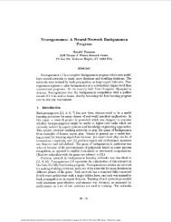
Fig. 1. Tracking error adaptive NN controller structure.<br />
Assumption 2 ensures that the function is bounded away<br />
from zero. The actual control input is selected as<br />
(18)<br />
where<br />
is the actual weights for the second NN.<br />
Substituting (17) and (18) into (16) yields<br />
where<br />
and<br />
(19)<br />
(20)<br />
(21)<br />
Equations (13) and (19) represent the closed-loop error dynamics.<br />
The next step is to design the NN weight tuning scheme<br />
such that the closed-loop system stability can be inferred.<br />
B. Weight Updates<br />
In tracking-error-based NN controller, two NNs are employed<br />
to approximate the nonlinear dynamics and their weights are<br />
tuned online using tracking errors. It is required to show the errors<br />
and and the NN weights and are<br />
bounded. To accomplish this, first, an assumption to define the<br />
bounds on the target weights and activation functions are presented.<br />
Second, a discrete-time online weight tuning algorithms<br />
is introduced so that closed-loop stability is inferred.<br />
Assumption 3: Both the target weights and the activation<br />
functions for all NNs are bounded by known positive values so<br />
that<br />
and (22)<br />
This assumption is used during the Lyapunov pro<strong>of</strong>.<br />
The proposed adaptive NN controller structure based on<br />
tracking errors as feedback variables is shown in Fig. 1. The<br />
desired and actual state <strong>of</strong> the first variable is utilized to obtain<br />
the error, which when combined with the output <strong>of</strong> the first<br />
NN generates the virtual control input. This virtual control<br />
input is combined with the second state to become the NN<br />
inputs for the second action NN. The second NN output along<br />
with the tracking error <strong>of</strong> the second state is considered as the<br />
input to the nonstrict feedback nonlinear discrete-time system.<br />
The tuning <strong>of</strong> the two NN weights is accomplished using the<br />
tracking errors.<br />
Theorem 1: Consider the system defined in (3) along with<br />
the Assumptions 1–3 hold. Let the disturbances and NN approximation<br />
errors be bounded, whose bounds are considered<br />
known as , , , and<br />
. Let the first NN weight tuning be given by<br />
with the second NN weights tuning be provided by<br />
(23)<br />
(24)<br />
where , , , and are design parameters.<br />
Let the virtual and actual control inputs be defined by (9)<br />
and (18), respectively. The tracking errors from (5) and<br />
from (11) and the NN weights estimates and<br />
are UUB, with the bounds specifically given by (A.8)–(A.11)<br />
provided the design parameters are selected as<br />
(25)<br />
(26)<br />
(27)<br />
(28)<br />
Pro<strong>of</strong>: See the Appendix.<br />
Remark 1: A well-defined controller is developed in this<br />
paper because a single NN in (7) and (17) is utilized to approximate<br />
a ratio <strong>of</strong> two unknown smooth nonlinear functions<br />
thereby avoiding the problem <strong>of</strong><br />
, becoming<br />
zero. This is in contrast from using a single NN for each <strong>of</strong> these<br />
individual functions consistent with the previous literature [6].<br />
Remark 2: The NN weight tuning proposed in (23) and (24)<br />
renders a semirecurrent NN due to the proposed weight tuning<br />
law even though a feedforward NN architecture is utilized. Here,
JAGANNATHAN AND HE: NN-BASED STATE FEEDBACK CONTROL OF A NONLINEAR DISCRETE-TIME SYSTEM 2077<br />
the NN outputs are not fed as delayed inputs to the network<br />
whereas the outputs <strong>of</strong> each layer are fed as delayed inputs to<br />
the same layer. This semirecurrent NN architecture renders a<br />
dynamic NN, which is capable <strong>of</strong> predicting the state one step<br />
ahead.<br />
Remark 3: It is only possible to show boundedness <strong>of</strong> all the<br />
closed-loop signals by using an extension <strong>of</strong> Lyapunov stability<br />
[6] due to the presence <strong>of</strong> approximation errors and bounded<br />
disturbances, a result consistent with the literature [4]–[6]. The<br />
controller gains and can be selected using (27) and (28)<br />
so that the closed-loop stability can be ensured.<br />
IV. ADAPTIVE CRITIC CONTROLLER DESIGN<br />
Next we present the development <strong>of</strong> an adaptive critic NN<br />
controller. Our objective is to design an NN controller for systems<br />
(1) and (2) such that: 1) all the signals in the closed-loop<br />
system remain UUB; 2) the state follows a desired trajectory<br />
; and 3) certain long term system performance<br />
index is optimized. Though the adaptive critic NN controller<br />
development uses the backstepping approach, the actual control<br />
methodology is different from the one introduced in Section III<br />
as given next.<br />
A. Design <strong>of</strong> the Virtual <strong>Control</strong> Input<br />
For simplicity, let us denote<br />
Because is an unknown function, the desired virtual<br />
control input in (37) cannot be implemented in practice.<br />
By utilizing the first action NN to approximate this unknown<br />
function , is given by<br />
(37)<br />
where<br />
is the input vector to the<br />
first action NN, and denote the constant<br />
ideal output- and hidden-layer weights, the hidden-layer<br />
activation function represents ,<br />
is the number <strong>of</strong> the nodes in the hidden layer, and<br />
is the approximation error. It is demonstrated in [11] that, if<br />
the hidden-layer weight is chosen initially at random and<br />
kept constant and the number <strong>of</strong> hidden-layer nodes is sufficiently<br />
large, the approximation error can be made<br />
arbitrarily small so that the bound<br />
holds<br />
for all because the activation function forms a basis.<br />
Consequently, the virtual control is taken as<br />
(38)<br />
and<br />
System (3) can be rewritten as<br />
(29)<br />
(30)<br />
(31)<br />
(32)<br />
(33)<br />
where<br />
is the actual output-layer weight matrix<br />
to be tuned. The hidden-layer weight is randomly chosen<br />
initially and kept constant. Define the weight estimation error<br />
by<br />
Define the error between and as<br />
Equation (37) can be rewritten using (39) as<br />
(39)<br />
(40)<br />
Define the tracking error as<br />
(34)<br />
Combining (40) with (41), we get<br />
(41)<br />
where is the desired trajectory and subscript “ ” is introduced<br />
to minimize confusion between the error signals <strong>of</strong> the<br />
two controllers developed in this paper. Using (32), (34) can be<br />
expressed as<br />
(35)<br />
By viewing as a virtual control input, a desired virtual<br />
control signal can be designed as<br />
(36)<br />
or, equivalently<br />
where<br />
B. Design <strong>of</strong> the <strong>Control</strong> Input<br />
Write the error from (40) as<br />
(42)<br />
(43)<br />
(44)<br />
where<br />
system (35).<br />
is a design constant selected to stabilize the error<br />
(45)
2078 <strong>IEEE</strong> TRANSACTIONS ON NEURAL NETWORKS, VOL. 19, NO. 12, DECEMBER 2008<br />
where is the future value <strong>of</strong> . To stabilize<br />
the above system, the desired control input is chosen as<br />
(46)<br />
where is the controller gain to stabilize system (45).<br />
Note that depends upon future states because<br />
depends upon the . We solve this noncausal problem<br />
by using the universal NN approximator. It can be clear that<br />
is a nonlinear function <strong>of</strong> system state , virtual<br />
control input , desired trajectory , and system<br />
error . Therefore, can be approximated using<br />
an NN. By taking<br />
as the input to the NN, can be approximated as<br />
(47)<br />
where and denote the constant ideal<br />
output- and hidden-layer weights, the hidden-layer activation<br />
function represents , is the<br />
number <strong>of</strong> the nodes in the hidden layer, and<br />
is<br />
the approximation error.<br />
The actual control input is selected as the output <strong>of</strong> the second<br />
action NN<br />
where<br />
is the actual output-layer weight.<br />
Substituting (46)–(48) into (45), we get<br />
(48)<br />
where is a predefined threshold. The utility function<br />
is viewed as the current system performance index;<br />
and refer to the good and poor tracking performance,<br />
respectively.<br />
The long term system performance measure or the strategic<br />
utility function is defined as<br />
(52)<br />
where and , and is the horizon. The term<br />
is viewed here as the long system performance measure<br />
because it is the sum <strong>of</strong> all future system performance indices.<br />
Equation (52) can also be expressed as<br />
, which is similar to the standard Bellman equation.<br />
D. Design <strong>of</strong> the Critic NN<br />
The critic NN is used to approximate the strategic utility function<br />
. We define the prediction error as<br />
where the subscript “ ” stands for the “critic,”<br />
(53)<br />
(54)<br />
is the critic signal,<br />
and<br />
represent the matrix <strong>of</strong> weight estimates,<br />
is the<br />
activation function vector in the hidden layer, is the number<br />
<strong>of</strong> the nodes in the hidden layer, and the critic NN input is given<br />
by<br />
. The objective function to be minimized by the<br />
critic NN is defined as<br />
(55)<br />
The weight update rule for the critic NN is a gradient-based<br />
adaptation, which is given by<br />
(49)<br />
where<br />
(50)<br />
Equations (43) and (49) represent the closed-loop error dynamics.<br />
The next step is to design the adaptive critic NN controller<br />
weight updating rules. The critic NN is trained online<br />
to approximate the strategic utility function (long term system<br />
performance index). The critic signal, with a potential for estimating<br />
the future system performance, is employed to tune the<br />
two action NNs to minimize the strategic utility function and the<br />
unknown system estimation errors so that closed-loop stability<br />
is inferred.<br />
C. The Strategic Utility Function<br />
The utility function is defined based on the current<br />
system errors and it is given by<br />
if<br />
otherwise<br />
(51)<br />
(56)<br />
where<br />
(57)<br />
or<br />
(58)<br />
where is the NN adaptation gain.<br />
E. Weight Updating Rule for the First Action NN<br />
The first action NN<br />
weight is tuned by minimizing<br />
the functional estimation error and the error between<br />
the desired strategic utility function<br />
and the<br />
critic signal . Define<br />
(59)
JAGANNATHAN AND HE: NN-BASED STATE FEEDBACK CONTROL OF A NONLINEAR DISCRETE-TIME SYSTEM 2079<br />
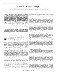
Fig. 2.<br />
Adaptive-critic-NN-based controller structure.<br />
where is defined in (44), , and the subscript<br />
“ ” stands for the “first action NN.” The value for the desired<br />
strategic utility function is taken as “0” [18], i.e., to indicate<br />
that at every step, the nonlinear system can track the reference<br />
signal well. Thus, (59) becomes<br />
(60)<br />
The objective function to be minimized by the first action NN<br />
is given by<br />
(61)<br />
The weight update rule for the action NN is also a gradientbased<br />
adaptation, which is defined as<br />
(62)<br />
where<br />
(63)<br />
or<br />
(64)<br />
where is the NN adaptation gain.<br />
The NN weight updating rule in (64) cannot be implemented<br />
in practice because the target weight is unknown. However,<br />
using (43), the functional estimation error is given by<br />
Substituting (65) into (64), we get<br />
(65)<br />
F. Weight Updating Rule for the Second Action NN<br />
Define<br />
(68)<br />
where is defined in (50), , and ,<br />
where the subscript “ ” stands for the “second action NN.”<br />
Following the similar design procedure and taking the bounded<br />
unknown disturbance and the NN approximation error<br />
to be zeros, the second action NN<br />
weight updating rule is given by<br />
(69)<br />
The proposed adaptive critic architecture based on weight<br />
tuning (67) and (69) with and is similar to supervised<br />
actor–critic architecture [10] wherein the supervisory<br />
signals and supply an additional source <strong>of</strong> evaluative<br />
feedback or reward that essentially simplifies the task<br />
faced by the learning system. As the actor gains pr<strong>of</strong>iciency,<br />
the supervisory signals are then gradually withdrawn to shape<br />
the learned policy towards optimality.<br />
To implement (69), the value <strong>of</strong> at the instant<br />
has to be known, which can be obtained by the following steps.<br />
1) Calculate , , , , , ,<br />
, and at the instant.<br />
2) Apply the control input to system (3) to obtain the<br />
states and .<br />
3) Use the tracking error definition to get as<br />
(70)<br />
(66)<br />
Assume that bounded disturbance and the NN approximation<br />
error are zeros for weight tuning implementation,<br />
then (66) is rewritten as<br />
(67)<br />
Equation (67) is the adaptive-critic-based weight updating rule<br />
for the first action NN<br />
. Next, we present the<br />
weight updating rule for the second action NN .<br />
4) Use the first action NN weight updating rule (66) to get<br />
.<br />
5) Once we have and , the value <strong>of</strong><br />
can be determined by using<br />
and<br />
(71)<br />
(72)<br />
The proposed adaptive critic NN controller is depicted in<br />
Fig. 2 based on the development given in this section. The desired<br />
and actual state <strong>of</strong> the first variable is utilized to obtain
2080 <strong>IEEE</strong> TRANSACTIONS ON NEURAL NETWORKS, VOL. 19, NO. 12, DECEMBER 2008<br />
the error, which when combined with the output <strong>of</strong> the first action<br />
NN generates the virtual control input. This virtual control<br />
input is combined with the second state and fed as inputs<br />
for the second action NN. The output <strong>of</strong> the second action NN<br />
becomes the input to the nonstrict feedback nonlinear discretetime<br />
system. The critic NN by using the states <strong>of</strong> the nonlinear<br />
system approximates the strategic utility function, which is subsequently<br />
employed to tune the NN weights <strong>of</strong> both action NNs.<br />
G. Stability Analysis<br />
Assumption 3 (Bounded Ideal Weights): Let , , and<br />
be the unknown output-layer target weights for the two action<br />
NNs and the critic NN and assume that they are bounded<br />
above so that<br />
and<br />
(73)<br />
where , , and represent<br />
the bounds on the unknown target weights where the Frobenius<br />
norm [11] is used.<br />
Fact 1: The activation functions are bounded by known positive<br />
values so that<br />
(74)<br />
where<br />
, is the upper bound for<br />
.<br />
Assumption 5 (Bounded NN Approximation Error): The NN<br />
reconstruction errors and are bounded<br />
over the compact set by and , respectively<br />
[6].<br />
Fact 1 and Assumption 5 are required during the Lyapunov<br />
pro<strong>of</strong>.<br />
Theorem 2: Consider the system given by (3). Let the Assumptions<br />
1–4 hold and the disturbance bounds and<br />
be known constants. Let the critic NN<br />
weight<br />
tuning be given by (58), the first action NN<br />
weight tuning provided by (67), and the second action NN<br />
weight tuning provided by (69). Given the virtual<br />
control input (38) and the control input (48),<br />
the tracking errors and and the NN weight estimates<br />
, , and are UUB, with the bounds<br />
specifically given by (A.26)–(A.28) provided the controller<br />
design parameters are selected as<br />
(a) (75)<br />
(b) (76)<br />
(c) (77)<br />
(d) (78)<br />
(e) (79)<br />
(f) (80)<br />
where , , and are NN adaptation gains, and<br />
are controller gains, and is employed to define the strategic<br />
utility function.<br />
Pro<strong>of</strong>: See the Appendix.<br />
Remark 4: The weight updates indicate that the critic NN and<br />
the functional approximation NNs have a semirecurrent architecture<br />
where the output from each node both in the input and<br />
output layers is fed back to the inputs.<br />
Remark 5: The mutual dependence between the two NNs (action-generating<br />
and critic NNs) in the adaptive critic NN architecture<br />
results in coupled tuning law equations because the critic<br />
output is utilized to tune the action NNs whereas the action<br />
NN outputs are utilized as inputs by the system to generate new<br />
states, which in turn are used by the critic NN. Moreover, additional<br />
complexities arise due to the addition <strong>of</strong> the second action<br />
NN because this addition causes further interaction among the<br />
three NNs. However, the Lyapunov stability analysis presented<br />
in the Appendix guarantees that the closed-loop system with all<br />
the three NNs is stable while ensuring the boundedness <strong>of</strong> all<br />
the signals.<br />
Remark 6: The weights <strong>of</strong> the action and critic NNs can be<br />
initialized at zero or random. This means that there is no explicit<br />
<strong>of</strong>fline learning phase needed in the proposed controller<br />
in contrast with the existing works where a preliminary <strong>of</strong>fline<br />
training phase is normally used.<br />
Remark 7: The proposed scheme results in a well-defined<br />
controller by avoiding the problem <strong>of</strong><br />
, becoming<br />
zero because a single NN is employed to approximate<br />
the ratio <strong>of</strong> two nonlinear smooth functions. Moreover, the controller<br />
gains and are selected using (78) and (79) to ensure<br />
closed-loop stability.<br />
Remark 8: Condition (78) can be verified easily. For instance,<br />
the hidden layer <strong>of</strong> the critic NN consists <strong>of</strong> nodes with the<br />
hyperbolic tangent sigmoid function as its activation function,<br />
then . The NN adaptation gain can be selected<br />
as<br />
to satisfy (78). Similar analysis can<br />
be performed to obtain the NN adaptation gains and .<br />
Remark 9: The number <strong>of</strong> hidden-layer neurons required for<br />
suitable approximation can be addressed by using the stability <strong>of</strong><br />
the closed-loop system and the error bounds <strong>of</strong> the NNs. From<br />
(75)–(80) and Remark 8, to stabilize the closed-loop system,<br />
the numbers <strong>of</strong> the hidden-layer nodes can be selected as<br />
, , and once the<br />
NN adaptation gains , , and are selected. However,<br />
to get a better approximation performance and according to<br />
[11], the hidden-layer nodes have to be selected large enough<br />
to make the approximation error approach zero. To balance<br />
stability and good approximation requirement, we start<br />
with a small number <strong>of</strong> nodes, and increase it until the controller<br />
achieves the satisfactory performance.<br />
Corollary 3: Given the hypothesis, the proposed adaptive<br />
critic NN controller, and the weight updating rules in Theorem<br />
2, the state approaches the desired virtual control input<br />
.<br />
Pro<strong>of</strong>: Combining (37) and (38), the difference between<br />
and is given by<br />
(81)<br />
where<br />
defined in (39) is the first action NN<br />
weight estimation error and<br />
is defined in (44). Be-
JAGANNATHAN AND HE: NN-BASED STATE FEEDBACK CONTROL OF A NONLINEAR DISCRETE-TIME SYSTEM 2081<br />
cause both and are bounded,<br />
is bounded to . In Theorem 2, we show that is<br />
bounded, i.e., the state is bounded to the virtual control<br />
signal . Thus, the state is bounded to the desired<br />
virtual control signal .<br />
Remark 10: Feedforward NNs are used as building blocks<br />
both in tracking error and adaptive-critic-based NN controllers.<br />
In the case <strong>of</strong> the first control methodology, tracking error is<br />
used as a feedback signal to tune the NN weights online. The<br />
only objective there is to reduce the tracking error, and therefore,<br />
no performance criterion is set. To the contrary, adaptive<br />
critic NN architectures use reinforcement learning signal generated<br />
by a critic NN. The critic signal can be generalized using<br />
complex optimization criteria including the variant <strong>of</strong> the standard<br />
Bellman equation. As a consequence, an adaptive critic<br />
NN architecture results in a considerable computational overhead<br />
due to the addition <strong>of</strong> a second NN for generating the<br />
critic signal. In the proposed work, a single NN is used to generate<br />
a critic signal for tuning the two action-generating NN<br />
weights. As a result, computational complexity is slightly reduced<br />
but still requires three NN when compared to two NN in<br />
the case <strong>of</strong> tracking-error-based NN controller. Moreover, all the<br />
NNs are tuned online compared to standard work in the adaptive<br />
critic NN literature [11]–[13]. Lyapunov-based analysis is<br />
demonstrated for stability whereas available adaptive critic papers<br />
use purely numerical simulation results without any analytical<br />
pro<strong>of</strong>s. Simulation results are presented in Section V to<br />
justify the theoretical conclusions.<br />
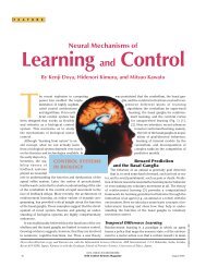
Fig. 3. Performance <strong>of</strong> a standard controller without NN.<br />
V. SIMULATIONS<br />
The purpose <strong>of</strong> the simulation is to verify the performance<br />
<strong>of</strong> the adaptive critic NN controller. Two cases are considered.<br />
The first is to apply the proposed adaptive critic NN controller<br />
to a nonlinear system. Then, a practical nonlinear system [e.g.,<br />
emission control in spark ignition (SI) engine] is considered and<br />
the proposed approach is employed.<br />
Example 1 (Adaptive Critic <strong>Control</strong>ler for Nonstrict <strong>Feedback</strong><br />
Nonlinear System): The control objective is to make the<br />
state follow the desired trajectory . The proposed<br />
adaptive critic NN controller is used on the following nonlinear<br />
system, given in nonstrict feedback form:<br />
(82)<br />
(83)<br />
where , are the states and is<br />
the control input. Note that both and include state<br />
.<br />
The reference signal was selected as<br />
, where and with a sampling interval <strong>of</strong><br />
. The total simulation time is taken as 250 s. The<br />
gains <strong>of</strong> the standard proportional controller are selected a priori<br />
and using (78) and (79).<br />
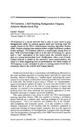
Fig. 4.<br />
<strong>Control</strong> input.<br />
NN1 , NN2 , and critic NN3 each<br />
consists <strong>of</strong> 15 nodes in the hidden layer. For weight updating,<br />
the learning rates are selected as , , and<br />
. All the initial weights are selected at random over<br />
an internal <strong>of</strong> and all the activation functions used are hyperbolic<br />
tangent sigmoid functions.<br />
Figs. 3 and 4 present the performance <strong>of</strong> the standard proportional<br />
controller alone from the adaptive critic controller and associated<br />
control input, respectively, without the NNs included.<br />
From Fig. 3, it is clear that the tracking performance has deteriorated<br />
in comparison with Fig. 5 when the NNs were included in<br />
the controller. Fig. 5 illustrates the superior performance <strong>of</strong> the<br />
adaptive critic NN controller. The gains were not altered in both<br />
simulations. Fig. 6 depicts the NN control input that appears<br />
to be sufficiently smooth such that it can be implemented in<br />
today’s embedded system hardware. Because the control input
2082 <strong>IEEE</strong> TRANSACTIONS ON NEURAL NETWORKS, VOL. 19, NO. 12, DECEMBER 2008<br />
SI engine operating at lean conditions. The engine dynamics<br />
can be expressed as a nonstrict feedback nonlinear discrete-time<br />
system <strong>of</strong> second order <strong>of</strong> the form [12]–[14] given by<br />
(84)<br />
(85)<br />
(86)<br />
(87)<br />
Fig. 5. Performance <strong>of</strong> the adaptive critic NN controller.<br />
Fig. 6. Adaptive critic NN control input.<br />
is bounded and according to (38) and (48), the NN weights are<br />
indeed bounded. The NNs are not trained <strong>of</strong>fline and the output<br />
layer weights are initialized at zero. Next, we present another<br />
simulation example where a practical nonlinear system is considered<br />
and the proposed controller is applied.<br />
Example 2 (Adaptive NN <strong>Control</strong>ler for SI Engines: A Practical<br />
Example): Lean operation <strong>of</strong> SI engine allows low emissions<br />
and improved fuel efficiency. However, at lean operation,<br />
the engine becomes unstable due to the cyclic dispersion<br />
in heat release. Literature shows that by controlling engines at<br />
lean operating conditions can reduce emissions as much as 60%<br />
[18] and it improves fuel efficiency by about 5% to 10%. Unfortunately,<br />
the engine exhibits strong cyclic dispersion, which<br />
causes instability. The simulation is designed to verify the performance<br />
<strong>of</strong> the proposed adaptive NN controller for the practical<br />
application, where the objective is to reduce cyclic dispersion.<br />
The adaptive NN controller is designed to stabilize the<br />
where and are the mass <strong>of</strong> air and fuel before th<br />
burn, respectively, is the unknown residual gas fraction,<br />
is the mass <strong>of</strong> fresh air fed per cycle, is the stoichiometric<br />
air–fuel ratio, , is the combustion efficiency,<br />
is the mass <strong>of</strong> fresh fuel per cycle, is the<br />
small changes in mass <strong>of</strong> fresh fuel per cycle, is the<br />
maximum combustion efficiency, which is a constant, is<br />
the equivalence ratio,<br />
are constant system parameters,<br />
and is the heat release in the th cycle. Because<br />
varies cycle by cycle, the engine is considered unstable without<br />
any control. In (56) and (57), and are unknown<br />
nonlinear functions <strong>of</strong> both and , so the system is a<br />
nonlinear discrete-time system <strong>of</strong> second order in nonstrict feedback<br />
form.<br />
Given Theorem 2 and Corollary 3 and using the pro<strong>of</strong> in [6],<br />
we could show that, with the proposed controller, both states can<br />
be bounded to their respective target values and . Then,<br />
the equivalence ratio (86) combustion efficiency<br />
(86), heat release (87), and the engine dynamics are stabilized.<br />
The cyclic dispersion is reduced when the variation in equivalence<br />
ratio<br />
is reduced, and this goal can be<br />
achieved by driving both states close enough to their desired<br />
target. The system parameters are selected as the following:<br />
, , , , ,<br />
, , , and .<br />
We add the unknown white noise with the deviation <strong>of</strong><br />
and to the and .<br />
The controller gains are selected as<br />
using<br />
(27) and (28). For weight updating, the adaptation gains are selected<br />
as and . The two NNs have 15<br />
hidden-layer nodes each. All the hidden-layer weights are selected<br />
uniformly within an interval <strong>of</strong> and all the activation<br />
functions are selected as hyperbolic tangent sigmoid functions.<br />
The cyclic dispersion observed at a lean equivalence ratio <strong>of</strong><br />
is presented in Fig. 7 when no control scheme is employed<br />
for 10 000 cycles. It shows that, without any control, the engine<br />
performance is unsatisfactory. Fig. 8 illustrates the performance<br />
<strong>of</strong> the NN controller. The dispersion is small and bounded and<br />
can be tolerable. Fig. 9 depicts the error between actual equivalence<br />
ratio and its desired value, which is bounded. Fig. 10<br />
displays the norm <strong>of</strong> the weights , , ,<br />
and . It is clear that the NN weights and the error<br />
converge and are bounded. The performance <strong>of</strong> a tuned conventional<br />
proportional and derivative controller is illustrated in [13]
JAGANNATHAN AND HE: NN-BASED STATE FEEDBACK CONTROL OF A NONLINEAR DISCRETE-TIME SYSTEM 2083<br />
Fig. 9. Error in equivalence ratio.<br />
Fig. 7. Cyclic dispersion without control.<br />
Fig. 8. Heat release with NN controller.<br />
and from the results in [13], the NN controller outperforms the<br />
conventional controllers. Next the proposed adaptive critic NN<br />
controller is applied.<br />
Adaptive Critic NN <strong>Control</strong>ler: The simulation parameters<br />
are selected as follows: 1000 cycles are considered at equivalence<br />
ratio <strong>of</strong> 0.71 with , , mass <strong>of</strong> new<br />
air , the standard deviation <strong>of</strong> mass <strong>of</strong> new fuel is ,<br />
, , the desired mass <strong>of</strong> air is taken as<br />
, and the desired mass <strong>of</strong> fuel is calculated as<br />
. A 5% unknown noise is<br />
added to the residual gas fraction as a way to include stochastic<br />
perturbation <strong>of</strong> system parameters. The gains <strong>of</strong> controllers are<br />
selected as , respectively, using (78) and (79).<br />
NN1 , NN2 , and critic NN3 each<br />
consists <strong>of</strong> 15 nodes in the hidden layer. For weight updating,<br />
the learning rates are selected as , , and<br />
. The initial weights are selected randomly over an<br />
internal <strong>of</strong> and all the activation functions are hyperbolic<br />
tangent sigmoid functions.<br />
Fig. 10 shows the cyclic dispersion without control now for<br />
1000 cycles at an equivalence ratio <strong>of</strong> . Here, the combustion<br />
process dynamics consisting <strong>of</strong> residual gas fraction and<br />
combustion efficiency are taken unknown. The cyclic dispersion<br />
is presented in Fig. 11, which indicates that, without any<br />
control, the engine performance is unsatisfactory. By contrast,<br />
Fig. 12 displays that the engine works satisfactorily at lean conditions,<br />
but the heat release appears to exhibit minimal dispersion.<br />
The overall controller performance appears to be satisfactory<br />
and fuel efficiency is 8% better than the standard adaptive<br />
NN controller due to optimal design.<br />
A comparison <strong>of</strong> the two controller approaches—a tracking<br />
error NN based and adaptive critic NN based—is shown in Example<br />
2 highlighting the differences, whereas in Example 1, an<br />
adaptive critic NN controller is compared with that <strong>of</strong> a standard<br />
controller. These clearly show that an adaptive critic NN controller<br />
is far superior even though it is computationally intensive<br />
than a tracking-error-based NN controller. On the other hand,<br />
Example 1 illustrates that a tracking-error-based NN controller<br />
performs better than a conventional controller. These clearly<br />
demonstrate that an adaptive critic NN controller renders a nearoptimal<br />
performance for a nonlinear discrete-time system in<br />
nonstrict feedback form.<br />
VI. CONCLUSION<br />
This paper proposes a novel adaptive critic NN controller to<br />
deliver a desired tracking performance for a class <strong>of</strong> discretetime<br />
nonstrict feedback nonlinear systems under the assumption<br />
that the states are available for measurement. A well-defined<br />
controller is developed since a single NN is utilized to<br />
approximate the ratio <strong>of</strong> two smooth nonlinear functions. Two<br />
NNs are employed for generating suitable control inputs in the<br />
case <strong>of</strong> tracking-error-based controller whereas three NNs are<br />
employed for the adaptive critic NN controller. The stability<br />
analysis <strong>of</strong> the closed-loop control system is introduced and the<br />
boundedness <strong>of</strong> the tracking error is demonstrated for both designs.<br />
The performance <strong>of</strong> the controller is demonstrated on a
2084 <strong>IEEE</strong> TRANSACTIONS ON NEURAL NETWORKS, VOL. 19, NO. 12, DECEMBER 2008<br />
Fig. 10. NN weight norms and error e (k).<br />
Fig. 11.<br />
Cyclic dispersion without control.<br />
practical nonlinear system. This paper proposes a novel adaptive<br />
NN controller to deliver a desired tracking performance for<br />
the control <strong>of</strong> a second-order unknown nonlinear discrete-time<br />
system in nonstrict feedback form. The NN controllers do not<br />
require an <strong>of</strong>fline learning phase and the weights can be initialized<br />
at zero or random. Results show that the performance <strong>of</strong><br />
Fig. 12.<br />
Cyclic dispersion with control.<br />
the proposed controllers is highly satisfactory while meeting the<br />
closed-loop stability.
JAGANNATHAN AND HE: NN-BASED STATE FEEDBACK CONTROL OF A NONLINEAR DISCRETE-TIME SYSTEM 2085<br />
APPENDIX<br />
Pro<strong>of</strong> <strong>of</strong> Theorem 1: Define the Lyapunov function candidate<br />
(A.1)<br />
where and are the upper bounds <strong>of</strong> function and<br />
, respectively, given a compact set (see Assumption 2), and<br />
, , and are design parameters (see Theorem 1).<br />
The first difference <strong>of</strong> Lyapunov function is given by<br />
(A.2)<br />
The first difference<br />
is obtained using (13) as<br />
(A.6)<br />
Combine (A.3), (A.4), (A.5), and (A.6) to get the first difference<br />
and simplify to get<br />
(A.3)<br />
Now take the second term in the first difference (A.1) and<br />
substitute (19) into (A.1) to get<br />
(A.4)<br />
Take the third term in (A.1) and substitute the weights updates<br />
from (23) and simplify to get<br />
(A.5)<br />
Take the fourth term in (A.1) and substitute the weights updates<br />
from (24) and simplify to get<br />
This implies that<br />
and<br />
(A.7)<br />
as long as (25) through (28) hold<br />
(A.8)
2086 <strong>IEEE</strong> TRANSACTIONS ON NEURAL NETWORKS, VOL. 19, NO. 12, DECEMBER 2008<br />
or<br />
or<br />
or<br />
where<br />
(A.9)<br />
(A.10)<br />
(A.11)<br />
(A.12)<br />
(A.18b)<br />
Taking the fourth term in (A.16) and substituting the weights<br />
updates from (69) and simplifying , we get<br />
According to a standard Lyapunov extension theorem [6], this<br />
demonstrates that the system tracking errors and the weight estimation<br />
errors are UUB. The boundedness <strong>of</strong> and<br />
implies that and are bounded, and this further<br />
implies that the weight estimates and are bounded.<br />
Therefore, all the signals in the closed-loop system are bounded.<br />
Pro<strong>of</strong> <strong>of</strong> Theorem 2: Define the Lyapunov function<br />
(A.19)<br />
Using the critic NN weights updating rule (58) to calculate<br />
the fifth and sixth item in (A.16), we obtain<br />
(A.13)<br />
where , are constants, is defined<br />
as<br />
(A.14)<br />
and<br />
is defined as<br />
(A.20)<br />
(A.21)<br />
Taking<br />
, and combining (A.17)–(A.21) to get the<br />
first difference <strong>of</strong> the Lyapunov function and simplifying it, we<br />
get<br />
(A.15)<br />
and , , and are the NN adaptation gains. The Lyapunov<br />
function consisting <strong>of</strong> the tracking errors and the weights<br />
estimation errors obviates the need for certainty equivalence assumption.<br />
The first difference <strong>of</strong> Lyapunov function is given by<br />
(A.16)<br />
The first difference<br />
is obtained using (43) as<br />
(A.17)<br />
Now taking the second term in the first difference (A.13) and<br />
substituting (49) into (A.16), we get<br />
where<br />
(A.22)<br />
(A.18a)<br />
Taking the third term in (A.16) and substituting the weights<br />
updates from (67) and simplifying, we get<br />
(A.23)<br />
Select<br />
(A.24)
JAGANNATHAN AND HE: NN-BASED STATE FEEDBACK CONTROL OF A NONLINEAR DISCRETE-TIME SYSTEM 2087<br />
This implies<br />
or<br />
or<br />
or<br />
or<br />
and<br />
as long as (75)–(80) hold and<br />
(A.25)<br />
(A.26)<br />
(A.27)<br />
(A.28)<br />
According to a standard Lyapunov extension theorem [6],<br />
this demonstrates that the system tracking error and the weight<br />
estimation errors are UUB. The boundedness <strong>of</strong> ,<br />
, and implies that , , and<br />
are bounded, and this further implies that the weight<br />
estimates , , and are bounded. Therefore,<br />
all the signals in the closed-loop system are bounded.<br />
REFERENCES<br />
[1] I. Kanellakopoulos, P. V. Kokotovic, and A. S. Morse, “Systematic<br />
design <strong>of</strong> adaptive controllers for feedback linearizable systems,” <strong>IEEE</strong><br />
Trans. Autom. <strong>Control</strong>, vol. 36, no. 11, pp. 1241–1253, Nov. 1991.<br />
[2] P. V. Kokotovic, “The joy <strong>of</strong> feedback: Nonlinear and adaptive,” <strong>IEEE</strong><br />
<strong>Control</strong> Syst. Mag., vol. 12, no. 3, pp. 7–17, Jun. 1992.<br />
[3] F. C. Chen and H. K. Khalil, “Adaptive control <strong>of</strong> nonlinear discretetime<br />
systems using neural networks,” <strong>IEEE</strong> Trans. Autom. <strong>Control</strong>, vol.<br />
40, no. 5, pp. 791–801, May 1995.<br />
[4] F. L. Lewis, S. Jagannathan, and A. Yesilderek, <strong>Neural</strong> <strong>Network</strong> <strong>Control</strong><br />
<strong>of</strong> Robot Manipulators and Nonlinear Systems. New York: Taylor<br />
and Francis, 1999.<br />
[5] F. L. Lewis, J. Campos, and R. Selmic, Neuro-Fuzzy <strong>Control</strong> <strong>of</strong> Industrial<br />
Systems With Actuator Nonlinearities. Philadelphia, PA: SIAM,<br />
2002.<br />
[6] S. Jagannathan, <strong>Neural</strong> <strong>Network</strong> <strong>Control</strong> <strong>of</strong> Nonlinear Discrete-Time<br />
Systems. Orlando, FL: CRC Press, 2006.<br />
[7] S. Jagannathan, “<strong>Control</strong> <strong>of</strong> a class <strong>of</strong> nonlinear discrete-time systems<br />
using multi layer neural networks,” <strong>IEEE</strong> Trans. <strong>Neural</strong> Netw., vol. 12,<br />
no. 5, pp. 1113–1120, Sep. 2001.<br />
[8] P. J. Werbos, “ADP: Goals, opportunities and principles,” in Handbook<br />
<strong>of</strong> Learning and Approximate Dynamic Programming, ser. Computational<br />
Intelligence, J. Si, A. G. Barto, W. B. Powell, and D. Wunsch,<br />
II, Eds. Piscataway, NJ: <strong>IEEE</strong> Press, 2004, pp. 3–44.<br />
[9] P. J. Werbos, “A menu <strong>of</strong> designs for reinforcement learning over time,”<br />
in <strong>Neural</strong> <strong>Network</strong>s for <strong>Control</strong>, W. T. Miller, R. S. Sutton, and P. J.<br />
Werbos, Eds. Cambridge, MA: MIT Press, 1991, pp. 67–95.<br />
[10] M. T. Rosenstein and A. G. Barto, “Supervised actor-critic reinforcement<br />
learning,” in Handbook <strong>of</strong> Learning and Approximate Dynamic<br />
Programming, ser. Computational Intelligence, J. Si, A. G. Barto, W.<br />
B. Powell, and D. Wunsch, II, Eds. Piscataway, NJ: <strong>IEEE</strong> Press, 2004,<br />
pp. 337–358.<br />
[11] B. Igelnik and Y. H. Pao, “Stochastic choice <strong>of</strong> basis functions in adaptive<br />
function approximation and the functional-link net,” <strong>IEEE</strong> Trans.<br />
<strong>Neural</strong> Netw., vol. 6, no. 6, pp. 1320–1329, Nov. 1995.<br />
[12] C. S. Daw, C. E. A. Finney, M. B. Kennel, and F. T. Connolly, “Observing<br />
and modeling nonlinear dynamics in an internal combustion<br />
engine,” Phys. Rev. E, Stat. Phys. Plasmas Fluids Relat. Interdiscip.<br />
Top., vol. 57, no. 3, pp. 2811–2819, 1997.<br />
[13] P. He and S. Jagannathan, “Neuroemission controller for reducing<br />
cyclic dispersion in lean combustion spark ignition engines,” Automatica,<br />
vol. 41, pp. 1133–1142, 2005.<br />
[14] T. Inoue, S. Matsushita, K. Nakanishi, and H. Okano, Toyota Lean<br />
Combustion System—The Third Generation System, ser. SAE Technical<br />
Papers. New York: SAE, 1993, Pub. 930873.<br />
[15] G. G. Lendaris and J. C. Neidhoefer, “Guidance in the use <strong>of</strong> adaptive<br />
critics for control,” in Handbook <strong>of</strong> Learning and Approximate<br />
Dynamic Programming, ser. Computational Intelligence, J. Si, A. G.<br />
Barto, W. B. Powell, and D. Wunsch, II, Eds. Piscataway, NJ: <strong>IEEE</strong><br />
Press, 2004, pp. 97–124.<br />
[16] J. J. Murray, C. Cox, G. G. Lendaris, and R. Saeks, “Adaptive dynamic<br />
programming,” <strong>IEEE</strong> Trans. Syst. Man Cybern. C, Appl. Rev., vol. 32,<br />
no. 2, pp. 140–153, May 2002.<br />
[17] D. P. Bertsekas and J. N. Tsitsiklis, Neuro-Dynamic Programming.<br />
Belmont, MA: Athena Scientific, 1996.<br />
[18] J. Si and Y. T. Wang, “On-line learning control by association and<br />
reinforcement,” <strong>IEEE</strong> Trans. <strong>Neural</strong> Netw., vol. 12, no. 2, pp. 264–276,<br />
Mar. 2001.<br />
[19] X. Lin and S. N. Balakrishnan, “Convergence analysis <strong>of</strong> adaptive<br />
critic based optimal control,” in Proc. Amer. <strong>Control</strong> Conf., 2000, pp.<br />
1929–1933.<br />
Sarangapani Jagannathan (S’89–M’89–SM’99)<br />
received the B.S. degree in electrical engineering<br />
from College <strong>of</strong> Engineering, Guindy, Anna University,<br />
Madras, India, in 1987, the M.S. degree<br />
in electrical engineering from the University <strong>of</strong><br />
Saskatchewan, Saskatchewan, Saskatoon, SK,<br />
Canada, in 1989, and the Ph.D. degree in electrical<br />
engineering from the University <strong>of</strong> Texas, San<br />
Antonio, in 1994.<br />
During 1986–1987, he was a Junior Engineer<br />
at Engineers India Limited, New Delhi, India, as<br />
a Research Associate and Instructor from 1990 to 1991, at the University <strong>of</strong><br />
Manitoba, Winnipeg, MB, Canada, and worked at Systems and <strong>Control</strong>s Research<br />
Division, Caterpillar Inc., Peoria, IL, as a Consultant during 1994–1998.<br />
During 1998–2001, he was at the University <strong>of</strong> Texas at San Antonio, and<br />
since September 2001, he has been at the University <strong>of</strong> Missouri, Rolla, where<br />
he is currently Rutledge-Emerson Distinguished Pr<strong>of</strong>essor in the Department<br />
<strong>of</strong> Electrical and Computer Engineering and Site Director for the NSF Industry/University<br />
Cooperative Research Center on Intelligent Maintenance<br />
Systems. He has coauthored more than 190 refereed conference and juried<br />
journal articles and several book chapters and three books entitled <strong>Neural</strong><br />
<strong>Network</strong> <strong>Control</strong> <strong>of</strong> Robot Manipulators and Nonlinear Systems (London,<br />
U.K.: Taylor & Francis, 1999), Discrete-Time <strong>Neural</strong> <strong>Network</strong> <strong>Control</strong> <strong>of</strong><br />
Nonlinear Discrete-Time Systems (Boca Raton, FL: CRC Press, 2006), and<br />
Wireless Ad Hoc and Sensor <strong>Network</strong>s: Performance, Protocols and <strong>Control</strong><br />
(Boca Raton, FL: CRC Press, 2007). He currently holds 17 patents and several<br />
are in process. His research interests include adaptive and neural network control,<br />
computer/communication/sensor networks, prognostics, and autonomous<br />
systems/robotics.<br />
Dr. Jagannathan received several gold medals and scholarships during his<br />
undergraduate program. He was the recipient <strong>of</strong> Region 5 <strong>IEEE</strong> Outstanding<br />
Branch Counselor Award in 2006, Faculty Excellence Award in 2006, St. Louis<br />
Outstanding Branch Counselor Award in 2005, Teaching Excellence Award in<br />
2005, Caterpillar Research Excellence Award in 2001, Presidential Award for<br />
Research Excellence at UTSA in 2001, National Science Foundation (NSF) CA-<br />
REER award in 2000, Faculty Research Award in 2000, Patent Award in 1996,<br />
and Sigma Xi “Doctoral Research Award” in 1994. He has served and currently<br />
serving on the program committees <strong>of</strong> several <strong>IEEE</strong> conferences. He is currently<br />
serving as the Associate Editor for the <strong>IEEE</strong> TRANSACTIONS ON CONTROL<br />
SYSTEMS TECHNOLOGY, the <strong>IEEE</strong> TRANSACTIONS ON NEURAL NETWORKS, the<br />
<strong>IEEE</strong> TRANSACTIONS ON SYSTEMS ENGINEERING, and on several program committees.<br />
He is a member <strong>of</strong> Tau Beta Pi, Eta Kappa Nu, and Sigma Xi and <strong>IEEE</strong><br />
Committee on Intelligent <strong>Control</strong>. He served as the Program Chair for the 2007<br />
<strong>IEEE</strong> International Symposium on Intelligent <strong>Control</strong>, and Publicity Chair for<br />
the 2007 International Symposium on Adaptive Dynamic Programming.<br />
Pingan He received the M.S. degree in electrical engineering from the University<br />
<strong>of</strong> Missouri, Rolla, in 2004.<br />
Currently, he is a <strong>Control</strong>s Engineer at GM Power Train Group, Troy MI. His<br />
research interests include power train control systems.<br />
Mr. He is a member <strong>of</strong> Society <strong>of</strong> Automotive Engineers.