Adaptive Critic Designs - Neural Networks, IEEE ... - IEEE Xplore

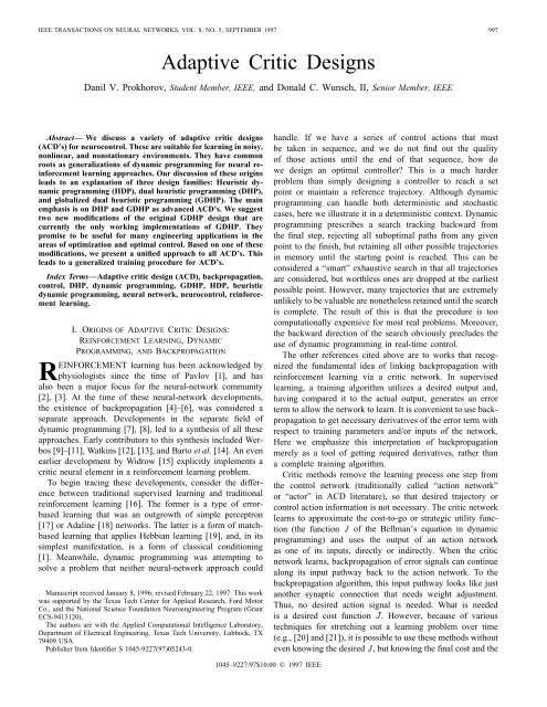
998 IEEE TRANSACTIONS ON NEURAL NETWORKS, VOL. 8, NO. 5, SEPTEMBER 1997one-step cost (or its estimate) further referred to as the utility. Thus, some of the architectures we will consider involvetime-delay elements.The work of Barto et al. [14] and that of Watkins [12]both feature table-look up critic elements operating in discretedomains. These do not have any backpropagation path to theaction network, but do use the action signals to estimate autility or cost function. Barto et al. use an adaptive criticelement for a pole-balancing problem. Watkins [12] createdthe system known as Q-learning (the name is taken from hisnotation), explicitly based on dynamic programming. Werboshas championed a family of systems for approximatingdynamic programming [10]. His approach generalizes previouslysuggested designs for continuous domains. For example,Q-learning becomes a special case of an action-dependentheuristic dynamic programming (ADHDP; note the actiondependentprefix AD used hereafter) in his family of systems.Werbos goes beyond a critic approximating just the function. His systems called dual heuristic programming (DHP)[23], and globalized dual heuristic programming (GDHP) [22]are developed to approximate derivatives of the functionwith respect to the states, and both and its derivatives,respectively. It should be pointed out that these systems donot require exclusively neural-network implementations: anydifferentiable structure suffices as a building block of thesystems.This paper focuses on DHP and GDHP and their AD formsas advanced ACD’s, although we start by describing simpleACD’s: HDP and ADHDP (Section II). We provide two newmodifications of GDHP that are easier to implement than theoriginal GDHP design. We also introduce a new design calledADGDHP, which is currently the topmost in the hierarchy ofACD’s (Section II-D). We show that our designs of GDHP andADGDHP provide a unified framework to all ACD’s, i.e., anyACD can be obtained from them by a simple reconfiguration.We propose a general training procedure for adaptation of thenetworks of ACD in Section III. We contrast the advancedACD’s with the simple ACD’s in Section IV. In Section V,we discuss results of experimental work.II. DESIGN LADDERA. HDP and ADHDPHDP and its AD form have a critic network that estimatesthe function (cost-to-go) in the Bellman equation of dynamicprogramming, expressed as follows:where is a discount factor for finite horizon problems, and is the utility function or local cost. Thecritic is trained forward in time, which is of great importancefor real-time operation. The critic network tries to minimizethe following error measure over time:(1)(2)(3)(a)(b)Fig. 1. (a) Critic adaptation in ADHDP/HDP. This is the same critic networkin two consecutive moments in time. The critic’s output J(t +1) is necessaryin order to give us the training signal J(t +1)+U(t), which is the targetvalue for J(t). (b) Action adaptation. R is a vector of observables, A is acontrol vector. We use the constant @J=@J =1as the error signal in orderto train the action network to minimize J.where stands for either a vector of observables ofthe plant (or the states, if available) or a concatenation ofand a control (or action) vector . [The configuration fortraining the critic according to (3) is shown in Fig. 1(a).] Itshould be noted that, although both anddepend on weights of the critic, we do not account for thedependence of on weights while minimizingthe error (2). For example, in the case of minimization inthe least mean squares (LMS) we could write the followingexpression for the weights’ update:where is a positive learning rate. 1We seek to minimize or maximize in the immediate futurethereby optimizing the overall cost expressed as a sum of allover the horizon of the problem. To do so we needthe action network connected as shown in Fig. 1(b). To geta gradient of the cost function with respect to the action’sweights, we simply backpropagate (i.e., the constant1) through the network. This gives us andfor all inputs in the vector and all the action’s weights ,respectively.In HDP, action-critic connections are mediated by a model(or identification) network approximating dynamics of theplant. The model is needed when the problem’s temporalnature does not allow us to wait for subsequent time stepsto infer incremental costs. When we are able to wait for thisinformation or when sudden changes in plant dynamics preventus from using the same model, the action network is directlyconnected to the critic network. This is called ADHDP.B. DHP and ADDHPDHP and its AD form have a critic network that estimatesthe derivatives of with respect to the vector . The critic1 There exists a formal argument on whether to disregard the dependence ofJ[Y (t+1)] on WC [24] or, on the contrary, to account for such a dependence[25]. The former is our preferred way of adapting WC throughout the papersince the latter seems to be more applicable for finite-state Markov chains [8].(4)

PROKHOROV AND WUNSCH: ADAPTIVE CRITIC DESIGNS 999network learns minimization of the following error measureover time:(5)where(6)whereis a vector containing partial derivatives ofthe scalar with respect to the components of the vector. The critic network’s training is more complicated than inHDP since we need to take into account all relevant pathwaysof backpropagation as shown in Fig. 2, where the paths ofderivatives and adaptation of the critic are depicted by dashedlines.In DHP, application of the chain rule for derivatives yieldswhere , and , are thenumbers of outputs of the model and the action networks,respectively. By exploiting (7), each of components of thevector from (6) is determined byAction-dependent DHP (ADDHP) assumes direct connectionbetween the action and the critic networks. However,unlike ADHDP, we still need to have a model network becauseit is used for maintaining the pathways of backpropagation.ADDHP can be readily obtained from our design of ADGDHPto be discussed in the Section II-D.The action network is adapted in Fig. 2 by propagatingback through the model down to the action. Thegoal of such adaptation can be expressed as follows:For instance, we could write the following expression for theweights’ update when applying the LMS training algorithm:whereis a positive learning rate.(7)(8)(9)(10)Fig. 2. Adaptation in DHP. This is the same critic network shown in twoconsecutive moments in time. The discount factor is assumed to be equalto 1. Pathways of backpropagation are shown by dashed lines. Componentsof the vector (t +1) are propagated back from outputs R(t +1)of themodel network to its inputs R(t) and A(t), yielding the first term of (7)and the vector @J(t +1)=@A(t), respectively. The latter is propagated backfrom outputs A(t) of the action network to its inputs R(t), completing thesecond term in (7). This corresponds to the left-hand backpropagation pathway(thicker line) in the figure. Backpropagation of the vector @U(t)=@A(t)through the action network results in a vector with components computedas the last term of (8). This corresponds to the right-hand backpropagationpathway from the action network (thinner line) in the figure. Following (8),the summator produces the error vector E2(t) used to adapt the critic network.The action network is adapted as follows. The vector (t +1)is propagatedback through the model network to the action network, and the resultingvector is added to @U(t)=@A(t). Then an incremental adaptation of the actionnetwork is invoked with the goal (9).C. GDHPGDHP minimizes the error with respect to both and itsderivatives. While it is more complex to do this simultaneously,the resulting behavior is expected to be superior. Wedescribe three ways to do GDHP (Figs. 3–5). The first of thesewas proposed by Werbos in [22]. The other two are our ownnew suggestions.Training the critic network in GDHP utilizes an errormeasure which is a combination of the error measures of HDPand DHP (2) and (5). This results in the following LMS updaterule for the critic’s weights:(11)where is given in (8), and and are positive learningrates.A major source of additional complexity in GDHPis the necessity of computing second-order derivatives. To get the adaptation signal-2 [the secondterm in (11)] in the originally proposed GDHP (Fig. 3), we firstneed to create a network dual to our critic network. The dualnetwork inputs the output and states of all hidden neurons ofthe critic. Its output,, is exactly what one wouldget performing backpropagation from the critic’s output toits input . Here we need these computations performedseparately and explicitly shown as a dual network. Then we

1000 IEEE TRANSACTIONS ON NEURAL NETWORKS, VOL. 8, NO. 5, SEPTEMBER 1997Fig. 3. Critic’s adaptation in the general GDHP design. X is a state vector ofthe network. 1 (Adaptation Signal-1) + 2 (Adaptation Signal-2) is the totaladaptation signal [see (11)]. The discount factor is assumed to be equal toone. According to (3), the summator at the upper center outputs the HDP-styleerror. Based on (6), the summator to the right produces the DHP-style errorvector. The mixed second-order derivatives @ 2 J(t)=@R(t)@WC are obtainedby finding derivatives of outputs @J(t)=@R(t) of the critic’s dual networkwith respect to the weights WC of the critic network itself. (This is symbolizedby the dashed arrow that starts from the encircled 1.) The multiplier performsa scalar product of the vector (6) with an appropriate column of the array@ 2 J(t)=@R(t)@WC, as illustrated by (16) in the Example.Fig. 4. Critic adaptation in our simplified GDHP design. Unlike GDHP inFig. 3, here we use explicit formulas to compute all necessary derivatives@ 2 J(t)=@R(t)@WC.can get the second derivatives sought by a straightforward butcareful backpropagation all the way down through the dualnetwork into the critic network. This is symbolized by thedashed line starting from the encircled 1 in Fig. 3.We have recently proposed and successfully tested a GDHPdesign with critic’s training based on deriving explicit formulasfor finding(Fig. 4) [28], and, tothe best of our knowledge, it is the first published successfulimplementation of GDHP [34]. While this design is morespecialized than the original one, its code is less complex,which is an important issue since correct implementation ofthe design of Fig. 3 is not a trivial task. We illustrate howto obtainfor the critic’s training of thisGDHP design in an example below.Finally, we have also suggested and are currently workingon the simplest GDHP design with a critic network as shownin Fig. 5 [42]. Here the burden of computing the secondderivativesis reduced to the minimum byexploiting a critic network with both scalar output of the estimateand vector output of . Thus, the second derivativesare conveniently obtained through backpropagation.We do not perform training of the action network throughinternal pathways of the critic network of Fig. 5 leading fromits output to the input because it would be equivalent togoing back to HDP. We already have high quality estimates ofas the critic’s outputs in the DHP portion of this GDHPdesign and therefore use them instead. 2 Thus, the action’straining is carried out only by the critic’s outputs,precisely as in DHP. However, the output implicitly affectsthe action’s training through the weights’ sharing in the critic.Of course, we do use the critic’s internal pathways from itsoutput to the input to train the action network in thedesigns of Figs. 3 and 4.Fig. 5.Critic network in a straightforward GDHP design.Example: This example illustrates how to calculate themixed second-order derivativesfor theGDHP design of Fig. 4. We consider a simple critic networkshown in Fig. 6. It consists of two sigmoidal neurons in itsonly hidden layer and a linear output . This network isequivalent to the following function:Derivatives , , are obtained as follows:(12)(13)where is the Kronecker delta. We can get the mixedsecond-order derivatives with respect to the weights of theoutput neuron as follows:(14)where , and . For the hidden layerneurons, the required derivatives are2 This situation is typical when ACD’s are used for optimal control. In otherapplication domains where the estimates of @J=@R obtained from the HDPportion of the design may be of a better quality than those of the DHP portion,the use of these more accurate estimates is preferable [40].(15)

PROKHOROV AND WUNSCH: ADAPTIVE CRITIC DESIGNS 1001Fig. 6. A simple network for the example of computing the second-orderderivatives @ 2 J(t)=@R(t)@W C in our GDHP design given in Fig. 4.where , , , and . Thus,based on (11), we can adapt weights in the network using thefollowing expression:(16)where the indexes and are chosen appropriately. Wealso assume that either,or since is a constantbias term.The example above can be easily generalized to largernetworks.It is clear that HDP and DHP can be readily obtainedfrom a GDHP design with the critic of Fig. 5. The simplicityand versatility of this GDHP design is very appealing, and itprompted us to a straightforward generalization of the criticof Fig. 5 for AD forms of ACD’s. Thus, we propose actiondependentGDHP (ADGDHP), to be discussed next.Fig. 7. Adaptation in ADGDHP. The critic network outputs the scalar Jand two vectors, R and A . The vector A (t +1)backpropagated throughthe action network is added to R (t +1). The vector R (t +1)propagatesback through the model, then it is is split in two vectors. One of them goestinto the square summator to be added to the vector @U(t)=@R(t) and tothe rightmost term in (18) (not shown). The second vector is added to thevector @U(t)=@R(t) in another summator. both of these summators producetwo appropriate error vectors E 2 (t), as in (19) and (20). According to (3),the right oval summator computes the error E 1 (t). Two error vectors E 2 (t)and the scalar E 1 (t) are used to train the critic network. The action networkis adap ted by the direct path A (t +1)between the critic and the actionnetworks.whereD. ADGDHPAs all AD forms of ACD’s, ADGDHP features a directconnection between the action and the critic networks. Fig. 7shows adaptation processes in ADGDHP. Although one couldutilize critics similar with those illustrated in Figs. 3 and 4, wefound ADGDHP easier to demonstrate when a critic akin toone of Fig. 5 is used. In addition, we gained versatility in thatthe design of Fig. 7 can be readily transformed into ADHDPor ADDHP.Consider training of the critic network. We can write(17)(18)and , are the numbers of outputs of the model and theaction networks, respectively.Based on (17) and (18), we obtain two error vectors,andfrom (6) as follows:(19)(20)As in GDHP, the critic network is additionally trained by thescalar error according to (3). If one applies the LMSalgorithm, it results in an update rule similar to (11).Fig. 7 also shows the direct adaptation pathbetween the action and the critic networks. We express the

1002 IEEE TRANSACTIONS ON NEURAL NETWORKS, VOL. 8, NO. 5, SEPTEMBER 1997goal of action’s training as follows:(21)Similar with what we stated in the Section II-C on GDHP,training of the action network is not carried out through theinternal pathways of the critic network leading from itsoutput to the input since it would be equivalent to returningto ADHDP. To train the action network, we use only thecritic’s outputs so as to meet (21). The goal (21) isthe same for all AD forms of ACD’s.III. GENERAL TRAINING PROCEDURE AND RELATED ISSUESThis training procedure is a generalization of that suggestedin [26], [30], [33], [38], and [43], and it is applicable toany ACD. It consists of two training cycles: critic’s andaction’s. We always start with critic’s adaptation alternating itwith action’s until an acceptable performance is reached. Weassume no concurrent adaptation of the model network, whichis previously trained offline, and any reasonable initializationfor and .In the critic’s training cycle, we carry out incremental optimizationof (2) and/or (5) by exploiting a suitable optimizationtechnique (e.g., LMS). We repeat the following operationstimes:for HDP, DHP, GDHP for ADHDP, ADDHP, ADGDHP1.0. Initialize t =0and R(0) Initialize t =0;R(0), and A(0)1.1. V (t) =f C [R(t);W C ] V(t)=f C [R(t);A(t);W C ]1.2. A(t) =f A [R(t);W A ] R(t+1)=f M [R(t);A(t);W M ]1.3. R(t +1)=A(t+1)=f A [R(t+1);W A ]f M [R(t);A(t);W M ]1.4. V (t +1)=f C [R(t+1);W C ] V(t+1)=f C [R(t+1);A(t+1);W C ]1.5. Compute E 1 (t);E 2 (t) from (2) and/or (5), and @V (t)=@W C ,tobeused in an optimization algorithm, then invoke the algorithm toperform one update of the critic’s weights W C . For the updateexample, see (4) and (11).1.6. t = t +1; continue from 1.1.Here stands for or , , ,andare the action, the critic and the modelnetworks, with their weights , respectively.In the action’s training cycle, we also carry out incrementallearning through an appropriate optimization routine, as in thecritic’s training cycle above. The list of operations for theaction’s training cycle is almost the same as that for the critic’scycle above (lines 1.0–1.6). However, we need to use (9) or(21), rather than (2) and/or (5); and instead ofbefore invoking the optimization algorithm forupdating the action’s weights [see (10) for the updateexample].The action’s training cycle should be repeated timeswhile keeping the critic’s weights fixed. We point outthat and are lengths of the corresponding trainingcycles. They are problem-dependent parameters of looselyspecified values. Ifwe can easily combineFig. 8. Test results of the autolander problem given for one of the mostchallenging cases where wind gusts were made 50% stronger than in standardconditions. After the ACD’s were trained on the number of landings shown,they were tested in 600 more trials, without any adaptation. Although theaverage training is much longer for GDHP and DHP than for HDP andADHDP, we could not observe an improvement of performance for eitherHDP or ADHDP if we continued their training further. Tight success meanslanding within a shortened touchdown region of the runway (it is the mostimportant characteristic). Loose success means landing within the limits ofthe standard runway. Similar results were obtained in various other flightconditions.both the cycles to avoid duplicating the computations in lines1.1–1.4. After the action’s training cycle is completed, onemay check action’s performance, then stop or continue thetraining procedure entering the critic’s training cycle again, ifthe performance is not acceptable yet. 3It is very important that the whole system consisting ofACD and plant would remain stable while both the networks ofACD undergo adaptation. Regarding this aspect of the trainingprocedure, we recommend to start the first training cycle ofthe critic with the action network trained beforehand to act asa stabilizing controller of the plant. Such a pretraining couldbe done on a linearized model of the plant (see, e.g., [45]).Bradtke et al. [26] proved that, in the case of the wellknownlinear quadratic regulation, a linear critic networkwith quadratic inputs trained by the recursive least squaresalgorithm in an ADHDP design converges to the optimal cost.If the regulator always outputs actions which are optimal withrespect to the target vector for the critic’s adaptation, i.e.,(22)where ,then the sequence is stabilizing, and it converges to theoptimal control sequence.Control sequences obtained through classical dynamic programmingare known to guarantee stable control, assuminga perfect match between the actual plant and its model usedin dynamic programming. Balakrishnan et al. [43] suggestedto stretch this fact over to a DHP-based ACD for linearand nonlinear control of systems with known models. Intheir design, one performs a training procedure similar to the3 Like many other training procedures, ours also implicitly assumes asufficiently varied set of training examples (e.g., different training trajectories)repeated often enough in order to satisfy persistent excitation—a property wellknown in a modern identification and adaptive control literature (see, e.g.,[37]).

PROKHOROV AND WUNSCH: ADAPTIVE CRITIC DESIGNS 1003above. Each training cycle is continued till convergence of thenetwork’s weights (i.e., , in the procedureabove). It is also suggested to use a new randomly chosenon every return to the beginning of the critic’s training cycle(line 1.6 is modified as follows: ; continue from 1.0).It is argued that whenever the action’s weights converge onehas a stable control, and such a training procedure eventuallyfinds the optimal control sequence.While theory behind classical dynamic programming demandschoosing the optimal vector of (22) for eachtraining cycle of the action network, we suggest incrementallearning of the action network in the training procedure above.A vector produced at the end of the action’s trainingcycle does not necessarily match the vector . However,our experience [28], [30], [44], [46], along with successfulresults in [33], [38], and [43], indicates that choosingprecisely is not critical.No training procedure currently exists that explicitly addressesissues of an inaccurate or uncertain model .It appears that model network errors of as much as 20%are tolerable, and ACD’s trained with such inaccurate modelnetworks are nevertheless sufficiently robust [30]. Althoughit seems consistent with assessments of robustness of conventionalneurocontrol (model-reference control with neuralnetworks) [31], [32], further research on robustness of controlwith ACD is needed, and we are currently pursuing this work.To allow using the training procedure above in presenceof the model network’s inaccuracies, we suggest to run themodel network concurrently with the actual plant or anothermodel, which imitates the plant more accurately than the modelnetwork but, unlike this network, it is not differentiable. Theplant’s outputs are then fed into the model network every sooften (usually, every time step) to provide necessary alignmentsand prevent errors of multiple-step-ahead predictionsfrom accumulating. Such a concurrently running arrangementis known under different names including teacher forcing[35] and series-parallel model [36]. After this arrangementis incorporated in an ACD, the critic will usually inputthe plant’s outputs, rather than the predicted ones from themodel network. Thus, the model network is mainly utilizedto calculate the auxiliary derivativesand.IV. SIMPLE ACD’S VERSUS ADVANCED ACD’SThe use of derivatives of an optimization criterion, ratherthan the optimization criterion itself, is known as being themost important information to have in order to find an acceptablesolution. In the simple ACD’s, HDP, and ADHDP,this information is obtained indirectly: by backpropagationthrough the critic network. It has a potential problem of beingtoo coarse since the critic network in HDP is not trained toapproximate derivatives of directly. An approach to improveaccuracy of this approximation has been proposed in [27]. It issuggested to explore a set of trajectories bordering a volumearound the nominal trajectory of the plant during the critic’straining, rather than the nominal trajectory alone. In spite ofthis enhancement, we still expect better performance from theadvanced ACD’s.Furthermore, Baird [39] showed that the shorter the discretizationinterval becomes, the slower the training of AD-HDP proceeds. In continuous time, it is completely incapableof learning.DHP and ADDHP have an important advantage over thesimple ACD’s since their critic networks build a representationfor derivatives of by being explicitly trained on themthrough and . For instance, in thearea of model-based control we usually have a sufficientlyaccurate model network and well-definedand. To adapt the action network we ultimately needthe derivatives or , rather than the functionitself. But an approximation of these derivatives is alreadya direct output of the DHP and ADDHP critics. Althoughmultilayer neural networks are well known to be universalapproximators of not only a function itself (direct output of thenetwork) but also its derivatives with respect to the network’sinputs (indirect output obtained through backpropagation) [41],we note that the quality of such a direct approximation isalways better than that of any indirect approximation for givensizes of the network and the training data. Work on a formalproof of this advantage of DHP and ADDHP is currently inprogress, but the reader is referred to the Section V for ourexperimental justification.Critic networks in GDHP and ADGDHP directly approximatenot only the function but also its derivatives. Knowingboth and its derivatives is useful in problems where availabilityof global information associated with the functionitself is as important as knowledge of the slope of , i.e., thederivatives of [40]. Besides, any shift of attention paid tovalues of or its derivatives during training can be readilyaccommodated by selecting unequal learning rates andin (11) (see Section II-C). In Section II-C we described threeGDHP designs. While the design of Fig. 5 seems to be themost straightforward and beneficial from the viewpoint ofsmall computational expenses, the designs of Figs. 3 and 4use the critic network more efficiently.Advanced ACD’s include DHP, ADDHP, GDHP, andADGDHP, the latter two being capable of emulating allthe previous ACD’s. All these designs assume availabilityof the model network. Along with direct approximation ofthe derivatives of , it contributes to a superior performanceof advanced ACD’s over simple ones (see the next Sectionfor examples of performance comparison). Although the finalselection among advanced ACD’s should certainly be basedon comparative results, we believe that in many applicationsthe use of DHP or ADDHP is quite enough. We also notethat the AD forms of the designs may have an advantage intraining recurrent action networks.V. EXPERIMENTAL STUDIESThis section provides an overview of our experimental workon applying various ACD’s to control of dynamic systems. Fordetailed information on interesting experiments carried out by

1004 IEEE TRANSACTIONS ON NEURAL NETWORKS, VOL. 8, NO. 5, SEPTEMBER 1997(a)(b)Fig. 9. Test results of two neurocontrollers for the ball-and-beam system. Edges of the beam correspond to 61, and its center is at zero. Dotted lines are thedesired ball positions x d (set points), solid lines are the actual ball trajectory x(t). (a) Conventional neurocontroller trained by the truncated backpropagationthrough time with NDEKF; (b) DHP action network tested on the same set points as in (a).other researchers in the field, the reader is referred to [33]and [43].The first problem deals with a simplified model of a commercialaircraft which is to be landed in a specified touchdownregion of a runway within given ranges of speed and pitchangle [22]. The aircraft is subject to wind disturbances thathave two components: wind shear (deterministic) and turbulentwind gusts (stochastic). To land safely, an external controllershould be developed to provide an appropriate sequence ofcommand elevator angles to the aircraft’s pitch autopilot.Along with actual states of the plane, a controller may alsouse desired values of the altitude and the vertical speedsupplied by an instrument landing system (ILS).To trade off between closely following the desired landingprofile from the ILS when far from the ground, and meetingthe landing constraints at the touchdown, one could use thefollowing utility function:(23)where , , are experimentally determined constants,and , , and are the actual altitude,vertical speed, and horizontal position of the plane. To avoida singularity at , we treat both terms as fixedto unity whenever ft.We found the problem with its original system of constraintsnot challenging enough since even the nonadaptivePID controller provided in [22] could solve it very well. Wecomplicated the problem by shortening the touchdown regionof the runway by 30%.We have compared the PID controller, ADHDP, HDP, andDHP for the same complicated version of the autolanderproblem. Implementation details are discussed in [28] and[30], and results are summarized in Fig. 8. The most importantconclusion is that in going from the simplest ACD, ADHDP,to the more advanced ACD’s one can attain a significantimprovement in performance.We have also applied DHP to control of actual hardware,a ball-and-beam system [44]. 4 The goal is to balance theball at an arbitrary specified location on the beam. We usethe recurrent multilayer perceptron for both model and actionnetworks. The model network inputs the current position of theball, , and the servo motor control signal, the latter beingthe only output of the action network with a sigmoidal outputnode. It predicts the next ball position, . The actionnetworks inputs from the model network and ,the desired ball position at the next time step. The critic4 Although we initially attempted an HDP design, we failed to make it work:its critic was not accurate enough to allow the action’s training.

PROKHOROV AND WUNSCH: ADAPTIVE CRITIC DESIGNS 1005(a)(b)(c)(d)Fig. 10. Performance of HDP [plots (a) and (b)] and DHP [(c) and (d)] for the MIMO plant. Dotted lines are the reference trajectories y1 3 and y3 2 , solidlines are the actual outputs y1(t) and y2(t). The rms error for DHP is 0.32 versus 0.68 for HDP.network uses and to produce an output,.We trained the action network off-line using a sufficientlyaccurate model network trained in the parallel identificationscheme [36]. We trained the DHP design according to thetraining procedure described in Section III. As the utility ,we have used the squared difference between and .Training was performed using the node-decoupled extendedKalman filter (NDEKF) algorithm [31]. The typical trainingtrajectory consisted of 300 consecutive points, with two orthree distinct desired locations of the ball. We were usuallyable to obtain an acceptable controller after three alternatingcritic’s and action’s training cycles. Starting with in(6), we moved on to and 0.9 for the second and thethird critic’s cycles, respectively.Fig. 9 shows a sample of performance of the DHP actionnetwork when tested on the actual ball-and-beam systemfor three set points not used in training. For comparison,performance of a conventional neurocontroller is also given.This neurocontroller of the same architecture as the actionnetwork was trained with the same model network by truncatedbackpropagation through time with NDEKF [32].Another example experiment deals with a nonlinearmultiple-input/multiple-output (MIMO) system proposed byNarendra and Mukhopadhyay [45] controlled by HDP andDHP designs [46]. This plant has three states, two inputs, andtwo outputs, and it is highly unstable for small input changes.The maximum time delay between the first control input andthe second output is equal to three time steps. The goal isto develop a controller to track two independent referencesignals as closely as possible.Although Narendra and Mukhopadhyay have explored severalcontrol cases, here we discuss only the case of fullyaccessible states and known plant equations. Thus, insteadof the model network, we utilize plant equations within theframework of both ACD’s.

1006 IEEE TRANSACTIONS ON NEURAL NETWORKS, VOL. 8, NO. 5, SEPTEMBER 1997The action network inputs the plant state variables, ,, and the desired plant outputs and, to be tracked by the actual plant outputsand, respectively. Since wehave different time delays for each control input/plant outputpair, we used the following utility:(24)The critic’s input vector consists of , ,, , , . Both the action and thecritic networks are simple feedforward multilayer perceptronswith one hidden layer of only six nodes. This is a much smallersize than that of the controller network used in [45], and weattribute our success in training to the NDEKF algorithm.The typical training procedure lasted three alternations ofcritic’s and action’s training cycles (see Section III). Theaction network was initially pretrained to act as a stabilizingcontroller [45], then the first critic’s cycle began within (6) on a 300-point trajectory.Fig. 10 shows our results for both HDP and DHP. Wecontinued training both designs until their performance wasno longer improving. The HDP action network performedmuch worse than its DHP counterpart. Although there is stillroom for improvement (e.g., using a larger network), we doubtthat HDP performance will ever be as good as that of DHP.Recently, KrishnaKumar [47] has reported HDP performancebetter than ours in Fig. 10(a) and (b). However, our DHPresults in Fig. 10(c) and (d) still remain superior. We thinkthat this is a manifestation of an intrinsically less accurateapproximation of the derivatives of in HDP, as stated inSection IV.VI. CONCLUSIONWe have discussed the origins of ACD’s as a conjunctionof backpropagation, dynamic programming, and reinforcementlearning. We have shown ACD’s through the design ladderwith steps varying in both complexity and power, from HDPto DHP, and to GDHP and its action-dependent form at thehighest level. We have unified and generalized all ACD’s viaour interpretation of GDHP and ADGDHP. Experiments withthese ACD’s have proven consistent with our assessment oftheir relative capabilities.ACKNOWLEDGMENTThe authors wish to thank Drs. P. Werbos and L. Feldkampfor stimulating and helpful discussions.REFERENCES[1] I. P. Pavlov, Conditional Reflexes: An Investigation of the PhysiologicalActivity of the Cerebral Cortex. London: Oxford Univ. Press, 1927.[2] S. Grossberg, “Pavlovian pattern learning by nonlinear neural networks,”in Proc. Nat. Academy Sci., 1971, pp. 828–831.[3] A. H. Klopf, The Hedonistic Neuron: A Theory of Memory, Learningand Intelligence. Washington, DC: Hemisphere, 1982.[4] P. J. Werbos, “Beyond regression: New tools for prediction and analysisin the behavioral sciences,” Ph.D. dissertation, Committee on Appl.Math., Harvard Univ., Cambridge, MA, 1974.[5] , The Roots of Backpropagation: From Ordered Derivatives toNeural Networks and Political Forecasting. New York: Wiley, 1994.[6] Y. Chauvin and D. Rumelhart, Eds., Backpropagation: Theory, Architectures,and Applications. Hillsdale, NJ: Lawrence Erlbaum, 1995.[7] R. E. Bellman, Dynamic Programming. Princeton, NJ: Princeton Univ.Press, 1957.[8] D. P. Bertsekas, Dynamic Programming: Deterministic and StochasticModels. Englewood Cliffs, NJ: Prentice-Hall, 1987.[9] P. J. Werbos, “The elements of intelligence,” Cybern., no. 3, 1968.[10] , “Advanced forecasting methods for global crisis warning andmodels of intelligence,” General Syst. Yearbook, vol. 22, pp. 25–38,1977.[11] , “Applications of advances in nonlinear sensitivity analysis,” inProc. 10th IFIP Conf. Syst. Modeling and Optimization, R. F. Drenickand F. Kosin, Eds. NY: Springer-Verlag, 1982.[12] C. Watkins, “Learning from delayed rewards,” Ph.D. dissertation, CambridgeUniv., Cambridge, U.K., 1989.[13] C. Watkins and P. Dayan, “Q-learning,” Machine Learning, vol. 8, pp.279–292, 1992.[14] A. G. Barto, R. S. Sutton, and C. W. Anderson, “Neuronlike elementsthat can solve difficult learning control problems,” IEEE Trans. Syst.,Man, Cybern., vol. SMC-13, pp. 835–846, 1983.[15] B. Widrow, N. Gupta, and S. Maitra, “Punish/reward: Learning with acritic in adaptive threshold systems,” IEEE Trans. Syst., Man, Cybern.,vol. SMC-3, pp. 455–465, 1973.[16] R. S. Sutton, Reinforcement Learning. Boston, MA: Kluwer, 1996.[17] F. Rosenblatt, Principles of Neurodynamics. Washington, D.C.: Spartan,1962.[18] B. Widrow and M. Lehr, “30 years of adaptive neural networks:Perceptron, madaline, and backpropagation,” Proc. IEEE, vol. 78, no.9, pp. 1415–1442, 1990.[19] D. O. Hebb, The Organization of Behavior. New York: Wiley, 1949.[20] R. S. Sutton, “Learning to predict by the methods of temporal differences,”Machine Learning, vol. 3, pp. 9–44, 1988.[21] P. J. Werbos, “Backpropagation through time: What it is and how to doit,” Proc. IEEE, vol. 78, no. 10, pp. 1550–1560, 1990.[22] W. T. Miller, R. S. Sutton, and P. J. Werbos, Eds., Neural Networks forControl. Cambridge, MA: MIT Press, 1990.[23] D. A. White and D. A. Sofge, Eds., Handbook of Intelligent Control:Neural, Fuzzy, and Adaptive Approaches. New York: Van NostrandReinhold, 1992.[24] P. J. Werbos, “Consistency of HDP applied to a simple reinforcementlearning problem,” Neural Networks, vol. 3, pp. 179–189, 1990.[25] L. Baird, “Residual algorithms: Reinforcement learning with functionapproximation,” in Proc. 12th Int. Conf. on Machine Learning, SanFrancisco, CA, July 1995, pp. 30–37.[26] S. J. Bradtke, B. E. Ydstie, and A. G. Barto, “Adaptive linear quadraticcontrol using policy iteration,” in Proc. Amer. Contr. Conf., Baltimore,MD, June 1994, pp. 3475–3479.[27] N. Borghese and M. Arbib, “Generation of temporal sequences usinglocal dynamic programming,” Neural Networks, no. 1, pp. 39–54, 1995.[28] D. Prokhorov, “A globalized dual heuristic programming and its applicationto neurocontrol,” in Proc. World Congr. Neural Networks,Washington, D.C., July 1995, pp. II-389–392.[29] D. Prokhorov and D. Wunsch, “Advanced adaptive critic designs,” inProc. World Congress on Neural Networks, San Diego, CA, Sept. 1996,pp. 83–87.[30] D. Prokhorov, R. Santiago, and D. Wunsch, “Adaptive critic designs:A case study for neurocontrol,” Neural Networks, vol. 8, no. 9, pp.1367–1372, 1995.[31] G. Puskorius and L. Feldkamp, “Neurocontrol of nonlinear dynamicalsystems with Kalman filter trained recurrent networks,” IEEE Trans.Neural Networks, vol. 5, pp. 279–297, 1994.[32] G. Puskorius, L. Feldkamp, and L. Davis, “Dynamic neural-networkmethods applied to on-vehicle idle speed control,” Proc. IEEE, vol. 84,no. 10, pp. 1407–1420, 1996.[33] F. Yuan, L. Feldkamp, G. Puskorius, and L. Davis, “A simple solutionto the bioreactor benchmark problem by application of Q-learning,” inProc. World Congr. Neural Networks, Washington, D.C., July 1995, pp.II-326–331.[34] P. J. Werbos, “Optimal neurocontrol: Practical benefits, new resultsand biological evidence,” in Proc. World Congr. Neural Networks,Washington, D.C., July 1995, pp. II-318–325.[35] R. Williams and D. Zipser, “A learning algorithm for continually runningfully recurrent neural networks,” Neural Computa., vol. 1, pp. 270–280.[36] K. S. Narendra and K. Parthasarathy, “Identification and control of dynamicalsystems using neural networks,” IEEE Trans. Neural Networks,vol. 1, pp. 4–27.

PROKHOROV AND WUNSCH: ADAPTIVE CRITIC DESIGNS 1007[37] K. S. Narendra and A. M. Annaswamy, Stable Adaptive Systems.Englewood Cliffs, NJ: Prentice-Hall, 1989.[38] R. Santiago and P. J. Werbos, “A new progress toward truly brain-likecontrol,” in Proc. World Congr. Neural Networks, San Diego, CA, June1994, pp. I-27–33.[39] L. Baird, “Advantage updating,” Wright Lab., Wright Patterson AFB,Tech. Rep. WL-TR-93-1146, Nov. 1993.[40] S. Thrun, Explanation-Based Neural Network Learning: A LifelongLearning Approach. Boston, MA: Kluwer, 1996.[41] H. White and A. Gallant, “On learning the derivatives of an unknownmapping with multilayer feedforward networks,” Neural Networks, vol.5, pp. 129–138, 1992.[42] D. Wunsch and D. Prokhorov, “Adaptive critic designs,” in ComputationalIntelligence: A Dynamic System Perspective, R. J. Marks, II, etal., Eds. New York: IEEE Press, 1995, pp. 98–107.[43] S. N. Balakrishnan and V. Biega, “Adaptive critic based neural networksfor control,” in Proc. Amer. Contr. Conf., Seattle, WA, June 1995, pp.335–339.[44] P. Eaton, D. Prokhorov, and D. Wunsch, “Neurocontrollers for ball-andbeamsystems,” in Intelligent Engineering Systems Through ArtificialNeural Networks 6 (Proc. Conf. Artificial Neural Networks in Engineering),C. Dagli et al., Eds. New York: Amer Soc. Mech. Eng. Press,1996, pp. 551–557.[45] K. S. Narendra and S. Mukhopadhyay, “Adaptive control of nonlinearmultivariable systems using neural networks,” Neural Networks, vol. 7,no. 5, pp. 737–752, 1994.[46] N. Visnevski and D. Prokhorov, “Control of a nonlinear multivariablesystem with adaptive critic designs,” in Intelligent Engineering SystemsThrough Artificial Neural Networks 6 (Proc. Conf. Artificial NeuralNetworks in Engineering), C. Dagli et al., Eds. NY: Amer. Soc. Mech.Eng. Press, 1996, pp. 559–565; note misprints in rms error values.[47] K. KrishnaKumar, “Adaptive critics: Theory and applications,” tutorialat Conf. Artificial Neural Networks in Engineering (ANNIE’96), St.Louis, MO, Nov. 10–13, 1996.Donald C. Wunsch, II (SM’94) completed a HumanitiesHonors Program at Seattle University, WA,in 1981 and received the B.S. degree in appliedmathematics from the University of New Mexico,Albuquerque, in 1984, the M.S. degree in appliedmathematics and the Ph.D. degree in electrical engineeringfrom the University of Washington, Seattle,in 1987 and 1991, respectively.He was Senior Principal Scientist at Boeing,Seattle, WA, where he invented the first optical implementationof the ART1 neural network, featuredin the 1991 Annual Report, and other optical neural networks and appliedresearch contributions. He has also worked for International Laser Systemsand Rockwell International, both at Kirtland AFB, Albuquerque, NM. He isDirector of the Applied Computational Intelligence Laboratory at Texas TechUniversity, Lubbock, TX, involving six other faculty, several postdoctoralassociates, doctoral candidates, and other graduate and undergraduate students.His current research includes neural optimization, forecasting, and control,financial engineering, fuzzy risk assessment for high-consequence surety, windengineering, characterization of the cotton manufacturing process, intelligentagents, and Go. He is heavily involved in research collaborations with formerSoviet scientists.Dr. Wunsch is an Academician in the International Academy of TechnologicalCybernetics and the International Informatization Academy. He isrecipient of the Halliburton Award for excellence in teaching and research atTexas Tech. He is a member of the International Neural Network Society anda past member of the IEEE Neural Network Council.Danil V. Prokhorov (S’95) received the HonorsDiploma in Robotics from the State Academy ofAerospace Instrument Engineering (formerly LIAP),St. Petersburg, Russia, in 1992. He is currently completingthe Ph.D. degree in electrical engineering atTexas Tech University, Lubbock, TX.He worked at the Institute for Informatics andAutomation of the Russian Academy of Sciences(formerly LIIAN), St. Petersburg, Russia, as a ResearchEngineer. He worked at the Research Laboratoryof Ford Motor Co., Dearborn, MI, as a SummerIntern in 1995–1997. His research interests are in adaptive critics, signalprocessing, system identification, control, and optimization based on variousneural networks.Mr. Prokhorov is a member of the International Neural Network Society.