Optimal Tracking Control for a Class of Nonlinear Discrete-Time ...

IEEE TRANSACTIONS ON NEURAL NETWORKS, VOL. 22, NO. 12, DECEMBER 2011 1851Optimal Tracking Control for a Class of NonlinearDiscrete-Time Systems with Time Delays Based onHeuristic Dynamic ProgrammingHuaguang Zhang, Senior Member, IEEE, Ruizhuo Song, Member, IEEE, Qinglai Wei, Member, IEEE,and Tieyan Zhang, Member, IEEEAbstract— In this paper, a novel heuristic dynamic programming(HDP) iteration algorithm is proposed to solve the optimaltracking control problem for a class of nonlinear discrete-timesystems with time delays. The novel algorithm contains stateupdating, control policy iteration, and performance index iteration.To get the optimal states, the states are also updated. Furthermore,the “backward iteration” is applied to state updating.Two neural networks are used to approximate the performanceindex function and compute the optimal control policy forfacilitating the implementation of HDP iteration algorithm. Atlast, we present two examples to demonstrate the effectiveness ofthe proposed HDP iteration algorithm.Index Terms— Adaptive dynamic programming, approximatedynamic programming, heuristic dynamic programming iteration,optimal control, time delays.I. INTRODUCTIONTIME delay often occurs in the transmission betweendifferent parts of systems. Transportation systems, communicationsystems, chemical processing systems, metallurgicalprocessing systems, and power systems are examplesof time delay systems [1]. So the investigation of time delaysystems is significant [2]–[7]. In addition, the tracking controlproblem is often encountered in industrial production. It hasbeen the focus of many researchers for many years [8]–[11].In [12], the optimal tracking control problem was studiedbased on dynamic output feedback for linear systems withtime delays in state and control. The optimal output trackingcontrol problem was discussed for a class of nonlinear systemsManuscript received June 29, 2010; revised September 27, 2011; acceptedOctober 5, 2011. Date of publication November 1, 2011; date of currentversion December 1, 2011. This work was supported in part by the NationalNatural Science Foundation of China under Grant 50977008, Grant 60821063,Grant 61034005, and Grant 60972164, and the National Basic ResearchProgram of China under Grant 2009CB320601.H. Zhang is with the School of Information Science and Engineering,Northeastern University, Shenyang 110004, China. He is also with theKey Laboratory of Integrated Automation of Process Industry (NortheasternUniversity) of the National Education Ministry, Shenyang 110004, China(e-mail: hgzhang@ieee.org).R. Song is with the School of Information Science and Engineering, NortheasternUniversity, Shenyang 110004, China (e-mail: ruizhuosong@163.com).Q. Wei is with the Key Laboratory of Complex Systems and IntelligenceScience, Institute of Automation, Chinese Academy of Sciences, Beijing100190, China (e-mail: qinglaiwei@gmail.com).T. Zhang is with the Department of Electrical Engineering, ShenyangInstitute of Engineering, Shenyang 110136, China (e-mail: zty@sie.edu.cn).Color versions of one or more of the figures in this paper are availableonline at http://ieeexplore.ieee.org.Digital Object Identifier 10.1109/TNN.2011.2172628with time delay in [13], and the optimal output trackingcontrol problem was transformed into a sequence of linearinhomogeneous two-point boundary value problems includingadjoint vector differential equations. In [14], multilayer neuralnetworks were used to design an optimal tracking neurocontrollerfor discrete-time nonlinear dynamic systems withquadratic cost function. However, the optimal tracking controlproblem for nonlinear discrete-time systems with time delaysthrough the framework of Hamilton–Jacobi–Bellman (HJB)equation is still very difficult to be handled.As is well known, dynamic programming is very usefulin solving the optimal control problems. However, due tothe “curse of dimensionality” of dynamic programming [15],[16], adaptive/approximate dynamic programming (ADP)algorithms have been paid much attention in order to obtainapproximate solutions of the HJB equation effectively.ADP was proposed by Werbos for discrete-time dynamicalsystems [17]. In recent years, ADP algorithms were furtherdeveloped by Lewis [18]–[20], Powell [21], Jagannathan[22], [23], Murray [24], Si [25]–[27], Liu [28], [29], andso on. In [30], Werbos classified ADP approaches into fourmain schemes: heuristic dynamic programming (HDP), dualheuristic dynamic programming (DHP), action-dependentHDP, and action-dependent DHP. HDP is the most basic andwidely applied structure of ADP [31], [32]. Moreover, somerecent research trends within the field of ADP and optimalfeedback control based on ADP were introduced in [33] and[34]. In [35], Bradtke, Ydestie, and Barto presented stabilityand convergence results for dynamic programming-basedreinforcement learning applied to linear quadratic regulation.Furthermore, a greedy iteration HDP scheme with convergenceproof was proposed for solving the optimal control problem fornonlinear discrete-time systems in [36]. In [37], a new type ofperformance index of optimal tracking problem was defined,and the infinite-time optimal tracking control problem for aclass of discrete-time nonlinear systems using HDP iterationalgorithm was solved. Additionally, the near-optimal controlproblem for a class of nonlinear discrete-time systems withcontrol constraints was solved by iteration ADP algorithmin [38].In spite of significant progress on HDP algorithm in theoptimal control field, within the radius of our knowledge, it isstill an open problem about how to solve the optimal trackingcontrol problem for nonlinear systems with time delays based1045–9227/$26.00 © 2011 IEEE

1852 IEEE TRANSACTIONS ON NEURAL NETWORKS, VOL. 22, NO. 12, DECEMBER 2011on HDP algorithm. In this paper, this open problem will beexplicitly figured out. First, the HJB equation for discrete timedelay system is derived which is based on state error andcontrol error. In order to solve this HJB equation, a noveliteration HDP algorithm containing state updating, controlpolicy iteration, and performance index function iteration isproposed. We also give the convergence proof for the noveliteration HDP algorithm. At last, two neural networks areused, the critic neural network and the action neural networkare devoted to approximate the performance index functionand the corresponding control policy, respectively. The maincontributions of this paper can be summarized as follows.1) It is the first time to solve the optimal tracking controlproblem for nonlinear systems with time delays usingHDP algorithm.2) For the novel HDP algorithm, in order to get the optimalstates, the state is also updated according to the controlpolicy.3) In the state update, we adopt “backward iteration.” Forthe (i + 1) th performance index function iteration, thestate at time step k +1 is updated according to the statesbefore time step k +1 inthei th iteration and the controlpolicy in the i th iteration.This paper is organized as follows. In Section II, wepresent the problem formulation. In Section III, the optimaltracking control scheme is developed based on iteration HDPalgorithm and the convergence proof is given. In Section IV,the neural network implementation for the tracking controlscheme is discussed. In Section V, two examples are given todemonstrate the effectiveness of the proposed control scheme.In Section VI, the conclusion is drawn.II. PROBLEM FORMULATIONConsider a class of discrete-time affine nonlinear systemswith time delaysx(k + 1) = f (x(k − σ 0 ), x(k − σ 1 ),...,x(k − σ m ))+ g(x(k − σ 0 ), x(k − σ 1 ),...,x(k − σ m ))u(k)x(k) = ε 1 (k), −σ m ≤ k ≤ 0 (1)where x(k−σ 0 ), x(k−σ 1 ),...,x(k−σ m ) ∈R n ,andx(k−σ 1 ),...,x(k − σ m ) are states of time delays. f (x(k − σ 0 ), x(k −σ 1 ),...,x(k − σ m )) ∈R n , g(x(k − σ 0 ), x(k − σ 1 ),...,x(k −σ m )) ∈R n×m and the input u(k) ∈R m . ε 1 (k) is the initialstate, σ i is the time delay, set 0 = σ 0

ZHANG et al.: OPTIMAL TRACKING CONTROL FOR A CLASS OF NONLINEAR DISCRETE-TIME SYSTEMS WITH TIME DELAYS BASED ON HDP 1853pseudoinverse of g can be obtained by the MATLAB functionG = pinv(g).2) Least Square Method [43]: As g(·)g −1 (·) = I, wehave(−1g −1 (·) = g (·)g(·)) T g T (·). (7)Introducing E(0, r 2 ) ∈R n×m into g(·), thenḡ(·) can beexpressed as follows:(ḡ(·) = g(·) + E 0, r 2) (8)where every element in E(0, r 2 ) is zero-mean Gaussian noise.So we can get(−1g −1 (·) = ḡ (·)ḡ(·)) T g T (·). (9)Then we sample K times, every time we take nm Gaussianpoints, so we have E i (0, r 2 ), i ∈{1, 2,...,K }, every elementin E i is a Gaussian sample point. Thus, we have G(·) =[ḡ 1 ,...,ḡ K ],whereḡ i = g + E i (0, r 2 ), i ∈{1, 2,...,K }.So we can get(−1g −1 (·) = G (·)G(·)) T g T (·). (10)3) Neural Network Method [44]: First, we let theback-propagation (BP) neural network be expressed asˆF(X, V, W) = W T σ(V T X), whereW and V are the weightsof the neural network and σ is the activation function. Second,we use the output ˆx(k + 1) of BP neural network toapproximate x(k +1). Thenwehave ˆx(k +1) = W T σ(V T X),where X =[x(k − σ 0 ),...,x(k − σ m ), u(k)]. We have knownthat (1) is an affine nonlinear system. So we can get g =(∂ ˆx(k + 1)/∂u). The equation g −1 = (∂u/∂ ˆx(k + 1)) can beestablished.So we can see that u s is existent and can be obtainedby (6). In this paper, we adopt Moore-Penrose pseudoinversetechnique to get g −1 (·) in simulation part.According to (2) and (3), we can easily obtain the followingsystem:e(k + 1) = f (e(k − σ 0 ) + η(k − σ 0 ),...,e(k − σ m )+ η(k − σ m )) + g(e(k − σ 0 ) + η(k − σ 0 ),...,e(k − σ m ) + η(k − σ m ))× (g −1 (η(k − σ 0 ),...,η(k − σ m ))× (S(η(k)) − f (η(k − σ 0 ),...,η(k − σ m )))+ v(k)) − S(η(k)),e(k) = ε(k), −σ m ≤ k ≤ 0 (11)where ε(k) = ε 1 (k) − ε 2 (k).So the aim for this paper is changed to get an optimalcontrol policy not only making (11) asymptotically stable butalso making the performance index function (4) minimal. Tosolve the optimal tracking problem in this paper, the followingdefinition and assumption are required.Definition 3 (Asymptotic Stability) [1]: An equilibrium statee = 0 for (11) is asymptotically stable if:1) it is stable, i.e., given any positive numbers k 0 and ɛ,there exists δ > 0, such that every solution of (11)satisfiesmax |e(k)| ≤ δ andk 0 ≤k≤k 0 +σ mmaxk 0 ≤k≤∞|e(k)| ≤ ɛ;2)for each k 0 > 0thereisaδ>0 such that every solutionof (11) satisfies max |e(k)| ≤ δ andk 0 ≤k≤k 0 +σ mlim e(k) = 0.k→∞Assumption 1: Given (11), for the infinite-time horizonproblem, there exists a control policy v(k), which satisfies:1) v(k) is continuous on ,ife(k−σ 0 ) = e(k−σ 1 ) =···=e(k − σ m ) = 0, then v(k) = 0;2) v(k) stabilizes (11);3) ∀e(−σ 0 ), e(−σ 1 ), e(−σ m ) ∈R n , J(e(0), v(0)) is finite.Actually, for nonlinear systems without time delays, if v(k)satisfies Assumption 1, then we can say that v(k) is anadmissible control. The definition of admissible control canbe seen in [36] and [45].In the following section we focus on the design of v(k).A. Derivation of the Iteration HDP AlgorithmIn (11), for time step k, J ∗ (e(k)) is used to denotethe optimal performance index function, i.e., J ∗ (e(k)) =inf J(e(k), v(k)),v(k) andv∗ (k) = arg inf J(e(k), v(k)).v(k) u∗ (k) =v ∗ (k) + u s (k) is the optimal control for (1). Let e ∗ (k) =x ∗ (k) − η(k), wherex ∗ (k) is used to denote the state underthe action of the optimal tracking control policy u ∗ (k).According to Bellman’s principle of optimality [1], J ∗ (e(k))should satisfy the following HJB equation:{J ∗ (e(k)) = inf e T (k)Qe(k) + v T (k)Rv(k)v(k)}+ J ∗ (e(k + 1))(12)the optimal controller v ∗ (k) should satisfy{v ∗ (k) = arg inf e T (k)Qe(k) + v T (k)Rv(k)v(k)}+ J ∗ (e(k + 1)) . (13)Here we define e ∗ (k) = x ∗ (k) − η(k) andx ∗ (k + 1) = f (x ∗ (k − σ 0 ),...,x ∗ (k − σ m ))+ g(x ∗ (k − σ 0 ),...,x ∗ (k − σ m ))× u ∗ (k), k = 0, 1, 2,...,x ∗ (k) = ε 1 (k) k =−σ m , −σ m−1 ,...,−σ 0 . (14)Then the HJB equation is written as follows:J ∗ (e ∗ (k)) = (e ∗ (k)) T Qe ∗ (k) + (v ∗ (k)) T Rv ∗ (k)+ J ∗ (e ∗ (k + 1)). (15)Remark 2: Of course, one can reduce (1) to a systemwithout time delay by defining a new (σ m + 1)n-dimensionalstate vector y(k) = (x(k), x(k − 1),...,x(k − σ m )). However,Chyung has pointed out that there are two major disadvantagesof this method in [46]. First, the resulting new system is a(σ m + 1)n-dimensional system increasing the dimension ofthe system by (σ m + 1) fold. Second, the new system maynot be controllable even if the original system is controllable.This causes the set of attainability to have an empty interiorwhich, in turn, introduces additional difficulties [46]–[48].

ZHANG et al.: OPTIMAL TRACKING CONTROL FOR A CLASS OF NONLINEAR DISCRETE-TIME SYSTEMS WITH TIME DELAYS BASED ON HDP 1855In the following part, we present the convergence analysisof the iteration about (21)–(28).B. Convergence Analysis of the Iteration HDP AlgorithmLemma 1: Let v [i] (k) { and J [i+1] (e [i] (k)) be expressed as(25) and (27), and let μ [i] (k) } be arbitrary sequence ofcontrol policy, [i+1] be defined by( ) ( T ( T [i+1] e [i] (k) = e (k)) [i] Qe [i] (k) + μ (k)) [i] Rμ [i]( (k))+ [i] e [i−1] (k + 1) , i ≥ 0. (29)Thus, if J [0] = [0] = 0, then J [i+1] (e [i] (k)) ≤ [i+1] (e [i] (k)) ∀e [i] (k).Proof: For given ε 1 (k)(−σ m ≤ k ≤ 0) of (1), it can bestraight forward from the fact that J [i+1] (e [i] (k)) is obtainedby the control input v [i] (k), while [i+1] (e [i] (k)) is a result ofarbitrary control input.Lemma 2: Let the sequence J [i+1] (e [i] (k)) be defined by(27), v [i] (k) is the control policy expressed as (25). There isan upper bound Y , such that 0 ≤ J [i+1] (e [i] (k)) ≤ Y , ∀e [i] (k).Proof: Let γ [i] (k) be any control policy that satisfiesAssumption 1. Let J [0] = P [0] = 0, and P [i+1] (e [i] (k)) isdefined ( as follows:) ( T ( TP [i+1] e [i] (k) = e (k)) [i] Qe [i] (k) + γ (k)) [i] Rγ [i]( (k))+ P [i] e [i−1] (k + 1) . (30)From (30), we can obtain( ) (TP [i] e [i−1] (k + 1) = e [i−1] (k + 1))Qe [i−1] (k + 1)(T+ γ [i−1] (k + 1))Rγ [i−1]( (k + 1))+ P [i−1] e [i−2] (k + 2) . (31)Thus we can get( ) ( TP [i+1] e [i] (k) = e (k)) [i] Qe [i] (k)( T+ γ (k)) [i] Rγ [i] (k)(T+ e [i−1] (k + 1))Qe [i−1] (k + 1)(T+ γ [i−1] (k + 1))Rγ [i−1] (k + 1)(T+ ···+ e [0] (k + i))Qe [0] (k + i)(T+ γ [0] (k + i))Rγ [0] (k + i). (32)For j = 0,...,i, welet(TL(k + j) = e [i− j] (k + j))Qe[i− j] (k + j)(T+ γ [i− j] (k + j))Rγ[i− j] (k + j). (33)Then (32) can further be written as follows:( )P [i+1] e [i] ∑(k) = i L(k + j). (34)j=0Furthermore, we can see that( )i∑∀i : P [i+1] e [i] (k) ≤ lim L(k + j). (35)i→∞Noting that { γ [i] (k) } satisfies Assumption 1, according to thethird condition of Assumption 1, there exists an upper boundY such thatlimi→∞j=0i∑L(k + j) ≤ Y. (36)j=0From Lemma 1 we ( can obtain) ( )∀i : J [i+1] e [i] (k) ≤ P [i+1] e [i] (k) ≤ Y. (37)Theorem 1: For (1), the iteration algorithm is as in(21)–(28), then we have J [i+1] (e [i] (k)) ≥ J [i] (e [i] (k)),∀e [i] (k).{ Proof: For convenience of analysis, define a new sequence [i] (e(k)) } as follows:( T [i] (e(k)) = e T (k)Qe(k) + v (k)) [i] Rv [i] (k)+ [i−1] (e(k + 1)) (38)with v [i] (k) defined by (25), [0] (e(k)) = 0.In the following part, we will prove [i] (e(k)) ≤J [i+1] (e(k)) by mathematical induction.First, we prove it holds for i = 0. Notice thatJ [1] (e(k)) − [0] (e(k)) = e T (k)Qe(k)( T+ v (k)) [0] Rv [0] (k) ≥ 0 (39)thus for i = 0, we haveJ [1] (e(k)) ≥ [0] (e(k)). (40)Second, we assume it holds for i, i.e., J [i] (e(k)) ≥ [i−1] (e(k)), for∀e(k).Then, from (26) and (38), we can getJ [i+1] (e(k)) − [i] (e(k))= J [i] (e(k + 1)) − [i−1] (e(k + 1)) ≥ 0 (41)the following inequality holds: [i] (e(k)) ≤ J [i+1] (e(k)). (42)Therefore, (42) is proved by mathematical induction, for∀e(k).On the other hand, from Lemma 1, we have ∀e [i] (k),J [i+1] (e [i] (k)) ≤ [i+1] (e [i] (k)). So we have J [i] (e(k)) ≤ [i] (e(k)).Therefore ∀e(k), wehaveJ [i] (e(k)) ≤ [i] (e(k)) ≤ J [i+1] (e(k)). (43)So, for ∀e [i] (k), wehave( )J [i+1] e [i] (k)( )≥ J [i] e [i] (k) . (44)

1856 IEEE TRANSACTIONS ON NEURAL NETWORKS, VOL. 22, NO. 12, DECEMBER 2011We let J L (e L (k)) = lim J [i+1] (e [i] (k)). Accordingly,i→∞v L (k) = limi→∞ v[i] (k) and e L (k) = limi→∞ e[i] (k) is the correspondingstates. Let x L (k) = e L (k) + η(k) and u L (k) =v L (k) + u s (k).In the following part, we will show that the performanceindex function J L (e L (k)) satisfies the corresponding HJBfunction, and it is the optimal performance index function.Theorem 2: If the performance index function J i+1 (e i (k))is defined by (27). Let J L (e L (k)) = lim J [i+1] (e [i] (k)).i→∞Let v L (k) = limi→∞ v[i] (k) and e L (k) = limi→∞ e[i] (k) is thecorresponding states. Then the following equation can beestablished:( ) ( T ( TJ L e L (k) = e (k)) L Qe L (k) + v (k)) L Rv L( (k))+ J L e L (k + 1) . (45)Proof: First, according to Theorem 1, we haveJ [i+1] (e [i] (k)) ≥ J [i] (e [i] (k)), ∀e [i] (k). So, we can obtain( ) ( TQe (TRvJ [i+1] e [i] (k) ≥ e (k)) [i] [i] (k)+ v (k)) [i−1] [i−1]( (k))+ J [i−1] e [i−1] (k + 1) . (46)Let i →∞,wehavev L (k) = limi→∞ v[i] (k) and( ) ( T ( TJ L e L (k) ≥ e (k)) L Qe L (k) + v (k)) L Rv L( (k))+ J L e L (k + 1) . (47){ On the other hand, for any i and arbitrary control policyμ [i] (k) } ,let [i+1] (e [i] (k)) be as (29). By Lemma 1, wehave( ) ( T ( TJ [i+1] e [i] (k) ≤ e (k)) [i] Qe [i] (k) + μ (k)) [i] Rμ [i]( (k))+ [i] e [i−1] (k + 1) . (48)Since μ [i] (k) in (48) is chosen arbitrarily. We let the controlpolicy {μ [i] (k)} ={v [i] (k)}, ∀i. So we can get( ) ( TJ [i+1] e [i] (k) ≤ e (k)) [i] Qe [i] (k) + (v [i] (k)) T Rv [i]( (k))+J [i] e [i−1] (k + 1) . (49)Let i →∞, and then we have( T ( TJ L (e L (k)) ≤ e (k)) L Qe L (k) + v (k)) L Rv L( (k))+J L e L (k + 1) . (50)Thus, combining (47) with (50), we have( ) ( T ( TJ L e L (k) = e (k)) L Qe L (k) + v (k)) L Rv L( (k))+J L e L (k + 1) . (51)Next, we give a theorem to demonstrate J L (e L (k)) =J ∗ (e ∗ (k)).Theorem 3: Let the performance index functionJ [i+1] (e [i] (k)) be defined as (27) and J L (e L (k)) =lim J [i+1] (e [i] (k)). J ∗ (e ∗ (k)) is defined as in (15). Then wei→∞have J L (e L (k)) = J ∗ (e ∗ (k)).Proof: According to the definition J ∗ (e(k)) =infv(k)J(e(k), v(k)), we know thatJ [i+1] (e(k)) ≥ J ∗ (e(k)). (52)So for ∀e [i] (k), wehave( )J [i+1] (e [i] (k)) ≥ J ∗ e [i] (k) . (53)Let i →∞, and then ( we have) ( )J L e L (k) ≥ J ∗ e L (k) . (54)infv(k)On the other hand, according to the definition J ∗ (e(k)) =J(e(k), v(k)), for any θ > 0 there exists a sequenceof control policy μ [i] (k), such that the associated performanceindex function [i+1] (e(k)) similar as (29) satisfies [i+1] (e(k)) ≤ J ∗ (e(k)) + θ. From Lemma 1, we can getSo we haveJ [i+1] (e(k)) ≤ [i+1] (e(k)) ≤ J ∗ (e(k)) + θ. (55)( ) ( )J [i+1] e [i] (k) ≤ J ∗ e [i] (k) + θ. (56)Let i →∞, and then ( we can obtain) ( )J L e L (k) ≤ J ∗ e L (k) + θ. (57)Noting that θ is chosen ( arbitrarily, we have) ( )J L e L (k) ≤ J ∗ e L (k) . (58)From (54) and (58), ( we can get) ( )J L e L (k) = J ∗ e L (k) . (59)From Theorem 2, we can see that J L (e L (k)) satisfies HJBequation, so we have v L (k) = v ∗ (k). From (14) and (28), wehave e L (k) = e ∗ (k). Then we draw conclusion J L (e L (k)) =J ∗ (e ∗ (k)).After that, we give a theorem to demonstrate the state errorsystem (11) is asymptotically stable, i.e., the system state x(k)follows η(k) asymptotically.The following lemma is necessary for the proof of stabilityproperty.Lemma 3: Define the performance index function sequence{J [i+1] (e [i] (k)) } as (27) with J [0] = 0, and the controlpolicy sequence { v [i] (k) } as (25). Then we have that for∀i = 0, 1,..., the performance index function J [i+1] (e [i] (k))is a positive definite function.Proof: The Lemma can be proved by the following threesteps.1) Show That Zero Is an Equilibrium Point for (11): Forthe autonomous system of (11), let e(k − σ 0 ) = e(k − σ 1 ) =···=e(k − σ m ) = 0, we have e(k + 1) = 0. According to thefirst condition of Assumption 1, when e(k −σ 0 ) = e(k −σ 1 ) =···=e(k − σ m ) = 0, we have v(k) = 0. So according to thedefinition of equilibrium state in [1], we can say that zero isan equilibrium point for (11).

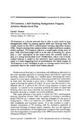
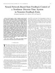
1858 IEEE TRANSACTIONS ON NEURAL NETWORKS, VOL. 22, NO. 12, DECEMBER 2011Fig. 1.J(e(k))v(k)Critic networkAction networku(k) = v(k) + u s(k)x(k+1) = f(x(k−σ 0),...,x(k−σ m))+g(x(k−σ 0),...,x(k−σ m))u(k)x(k+1)v(k)e(k)e(k)u s(k)e(k+1) = x(k+1) − η(k+1)Structure diagram of the algorithm.η(k+1) = s(η(k))η(k+1)IV. NEURAL NETWORK IMPLEMENTATION OF THEITERATION HDP ALGORITHMThe nonlinear optimal control solution relies on solving theHJB equation, exact solution of which is generally impossibleto be obtained for nonlinear time delay system. So we need touse parametric structures or neural networks to approximateboth control policy and performance index function. Therefore,in order to implement the HDP iterations, we employ neuralnetworks for approximations in this section.Assume the number of hidden layer neurons is denoted by l,the weight matrix between the input layer and hidden layer isdenoted by V , the weight matrix between the hidden layer andoutput layer is denoted by W, then the output of three-layerneural network is represented by( )ˆF(X, V, W) = W T σ V T X(64)where σ(V T X) ∈ R l is the sigmoid function. The gradientdescent rule is adopted for the weight update rules of eachneural network [26].Here, there are two networks, which are critic network andaction network, respectively. Both neural networks are chosenas three-layer BP network. The whole structure diagram isshowninFig.1.A. Critic NetworkThe critic network is used to approximate the performanceindex function J [i+1] (e(k)). The output of the critic networkis denoted as follows:( ) T ()Ĵ [i+1] (e(k)) = σ ) T e(k) . (65)w [i+1]c(v [i+1]cThe target function can be written as follows:J [i+1] (e(k)) = e T (k)Qe(k) + ( ˆv [i] (k) ) T R ˆv [i] (k)+Ĵ [i] (e(k + 1)). (66)Then we define the error function for the critic network asfollows:e c [i+1] (k) = Ĵ [i+1] (e(k)) − J [i+1] (e(k)). (67)The objective function to be minimized in the critic networkisE c [i+1] (k) = 1 (2e c (k)) [i+1] . (68)2So the gradient-based weights update rule for the criticnetwork is given bywherew c[i+2]v [i+2](k) = w c[i+1]c (k) = v c[i+1]w [i+1]cv [i+1]c(k) + w c[i+1] (k),(k) + v [i+1]c (k) (69)∂ E c(k) =−α [i+1] (k)c ,∂w c [i+1] (k)∂ E c(k) =−α [i+1]c∂v [i+1]c(k)(k)(70)and the learning rate α c of critic network is positive number.B. Action NetworkIn the action network, the states e(k − σ 0 ),...,e(k − σ m )are used as inputs to create the optimal control, ˆv [i] (k) asthe output of the network. The output can be formulated asfollows:( ) T ( )ˆv [i] (k) = w a[i] σ (v a [i] )T Y (k) (71)where Y (k) =[e T (k − σ 0 ),...,e T (k − σ m )] T .We define the output error of the action network as follows:e a [i] (k) =ˆv[i] (k) − v [i] (k). (72)The weights in the action network are updated to minimizethe following performance error measure:E a [i] (k) = 1 ( ) 2e a [i]2(k) . (73)The weights updating algorithm is similar to the one for thecritic network. By the gradient descent rule, we can obtainw a[i+1] (k) = w a [i] (k) + w a [i] (k),v a [i+1] (k) = v a [i] (k) + v a [i] (k) (74)wherew [i]a (k) =−α av [i]a (k) =−α a∂ E a [i] (k)∂w a [i] (k) ,∂ E [i]a (k)∂v [i]a (k)(75)and the learning rate α a of action network is positive number.V. SIMULATION STUDYIn this section, two examples are provided to demonstratethe effectiveness of the proposed iteration HDP algorithm inthis paper. One is about tracking chaotic signal, and the otheris about the situation that the function g(·) is noninvertible.

ZHANG et al.: OPTIMAL TRACKING CONTROL FOR A CLASS OF NONLINEAR DISCRETE-TIME SYSTEMS WITH TIME DELAYS BASED ON HDP 18591.511.51x 2η 2eta 20.50−0.5−1−1.5−1.5 −1 −0.5 0 0.5 1 1.5eta 1State trajectories0.50−0.5−1−1.50 10 20 30 40 50 60 70 80 90 100Time stepFig. 2.Hénon chaos orbits.Fig. 4. State variable trajectory x 2 and desired trajectory η 2 .State trajectories1.510.50−0.5−1−1.50 10 20 30 40 50 60 70 80 90 100Time stepx 1η 1Performance index function0.450.40.350.30.250.20.150.10.0500 5 10 15 20 25 30 35 40 45 50Iteration stepFig. 3. State variable trajectory x 1 and desired trajectory η 1 .Fig. 5.Convergence of performance index.A. Example 1Consider the following nonlinear time delay system whichis the example in [54] and [37] with modification:wherex(k + 1) = f (x(k), x(k − 1), x(k − 2))+ g(x(k), x(k − 1), x(k − 2))u(k)x(k) = ε 1 (k), −2 ≤ k ≤ 0 (76)f (x(k), x(k − 1), x(k − 2))[ 0.2x1 (k) exp (x=2 (k)) 2 ]x 2 (k − 2)0.3 (x 2 (k)) 2 x 1 (k − 1)and[ ]−0.2 0g(x(k), x(k − 1), x(k − 2)) =.0 −0.2The desired signal is well-known Hénon mapping as follows:[ ]η1 (k+1)η 2 (k+1)[1+b×η2 (k)−a×η1 2(k)η 1 (k)[ ]η1 (0)η 2 (0)=](77)where a = 1.4, b = 0.3,orbits are given as Fig. 2.Based on the implementation of proposed HDP algorithmin Section III-C, we first give the initial states as ε 1 (−2) =ε 1 (−1) = ε 1 (0) = [ 0.5 −0.5 ] T , and the initial control policyas β(k) = −2x(k). The implementation of the algorithmis at the time instant k = 3. The maximal iteration step= [ 0.1−0.1]. The chaotic signalError trajectories1.510.50−0.5−1−1.5−20 10 20 30 40 50 60 70 80 90 100Time stepFig. 6. Tracking error trajectories e 1 and e 2 .i max is 50. We choose three-layer BP neural networks asthe critic network and the action network with the structure2 − 8 − 1 and 6− 8 − 2, respectively. The iteration timeof the weights updating for two neural networks is 100.The initial weights are chosen randomly from [−0.1, 0.1],and the learning rate is α a = α c = 0.05. We selectQ = R = I 2 .The state trajectories are given as Figs. 3 and 4. The solidlines in the two figures are the system states, and the dashedlines are the trajectories of the desired chaotic signal. Fromthe two figures, we can see that the state trajectories of (76)follow the chaotic signal. From Lemma 2, Theorems 1 and 3,the performance index function sequence is bounded ande 1e 2

1860 IEEE TRANSACTIONS ON NEURAL NETWORKS, VOL. 22, NO. 12, DECEMBER 2011State trajectories10.80.60.40.20−0.2−0.4−0.6−0.8−10 10 20 30 40 50 60 70 80 90 100Time stepx 1η 1Performance index function0.70.650.60.550.50.450.40.350 20 40 60 80 100 120 140 160 180 200Iteration stepFig. 7. State variable trajectory x 1 and desired trajectory η 1 .Fig. 9.Convergence of performance index.State trajectories10.80.60.40.20−0.2−0.4−0.6−0.8−10 10 20 30 40 50 60 70 80 90 100Time stepFig. 8. State variable trajectory x 2 and desired trajectory η 2 .x 2η 2Error trajectories0.60.40.20−0.2−0.4−0.6−0.8−1−1.20 10 20 30 40 50 60 70 80 90 100Time stepFig. 10. Tracking error trajectories e 1 and e 2 .e 1e 2nondecreasing. Furthermore, it converges to the optimal performanceindex function as i →∞.ThecurveinFig.5showsthe properties of the performance index function sequence.According to Theorem 4, we know that (11) is asymptoticallystable. The error trajectories between (76) and Hénon chaoticsignal are presented in Fig. 6, and they converge to zeroasymptotically. It is clear that the new HDP iteration algorithmis very feasible.B. Example 2In this subsection, we consider the following nonlinear timedelay system:whereandx(k + 1) = f (x(k), x(k − 1), x(k − 2))+g(x(k), x(k − 1), x(k − 2))u(k)x(k) = ε 1 (k), −2 ≤ k ≤ 0 (78)f (x(k), x(k − 1), x(k − 2))[ ]0.2x1 (k) exp (x 2 (k)) 2 x 2 (k − 2)=0.3 (x 2 (k)) 2 x 1 (k − 1)g(x(k), x(k − 1), x(k − 2)) =[ ]x2 (k − 2) 0.0 1From (78), we know that g(·) is not always invertible.Here Moore-Penrose pseudoinverse technique is used to obtaing −1 (·).The desired orbit η(k) is generated by the followingexosystem:withA =η(k + 1) = Aη(k) (79)[ ] [ ]cos wT sin wT0, η(0) =− sin wT cos wT1where T = 0.1 s,w = 0.8π.At first, we give the initial states as ε 1 (−2) = ε 1 (−1) =ε 1 (0) = [ 0.5 −0.2 ] T , and the initial control policy as β(k) =−2x(k). We also implement the proposed HDP algorithm atthe time instant k = 3. The maximal iteration step i max is 60.The learning rate is α a = α c = 0.01, and other parameters inBP neural networks are the same as in Example 1. We selectQ = R = I 2 .The trajectories of the system states are presented in Figs. 7and 8. In the two figures, the solid lines are the system states,and the dashed lines are the desired trajectories. In addition,we give the curve of the performance index sequence in Fig. 9.It is bounded and convergent. It verifies Theorems 1 and 3 aswell. The tracking errors show in Fig. 10, which converge tozero asymptotically. It is clear that the tracking performance issatisfactory, and the new iteration algorithm proposed in thispaper is very effective.

ZHANG et al.: OPTIMAL TRACKING CONTROL FOR A CLASS OF NONLINEAR DISCRETE-TIME SYSTEMS WITH TIME DELAYS BASED ON HDP 1861VI. CONCLUSIONIn this paper, we proposed an effective HDP algorithmto solve optimal tracking problem for a class of nonlineardiscrete-time systems with time delays. First we defined aperformance index for time delay systems. Then a novel iterationHDP algorithm has been developed to solve the optimaltracking control problem. Two neural networks have been usedto facilitate the implementation of the iteration algorithm.Simulation examples have demonstrated the effectiveness ofthe proposed optimal tracking control algorithm.REFERENCES[1] M. Z. Manu and J. Mohammad, Time-Delay Systems Analysis, Optimizationand Applications. New York: North-Holland, 1987.[2] D. H. Chyung, “On the controllability of linear systems with delay incontrol,” IEEE Trans. Autom. Control, vol. 15, no. 2, pp. 255–257, Apr.1972.[3] D. H. Chyung, “Controllability of linear systems with multiple delaysin control,” IEEE Trans. Autom. Control, vol. 15, no. 6, pp. 694–695,Dec. 1970.[4] H. Y. Shao and Q. L. Han, “New delay-dependent stability criteriafor neural networks with two additive time-varying delay components,”IEEE Trans. Neural Netw., vol. 22, no. 5, pp. 812–818, May 2011.[5] J. P. Richard, “Time-delay systems: An overview of some recentadvances and open problems,” Automatica, vol. 39, no. 10, pp. 1667–1694, Oct. 2003.[6] S. C. Tong, Y. M. Li, and H. G. Zhang, “Adaptive neural networkdecentralized backstepping output-feedback control for nonlinear largescalesystems with time delays,” IEEE Trans. Neural Netw., vol. 22,no. 7, pp. 1073–1086, Jul. 2011.[7] V. N. Phat and H. Trinh, “Exponential stabilization of neural networkswith various activation functions and mixed time-varying delays,” IEEETrans. Neural Netw., vol. 21, no. 7, pp. 1180–1184, Jul. 2010.[8] Y. J. Liu, C. L. P. Chen, G.-X. Wen, and S. C. Tong, “Adaptive neuraloutput feedback tracking control for a class of uncertain discrete-timenonlinear systems,” IEEE Trans. Neural Netw., vol. 22, no. 7, pp. 1162–1167, Jul. 2011.[9] M. Wang, S. S. Ge, and K. S. Hong, “Approximation-based adaptivetracking control of pure-feedback nonlinear systems with multipleunknown time-varying delays,” IEEE Trans. Neural Netw., vol. 21,no. 11, pp. 1804–1816, Nov. 2010.[10] W. S. Chen and L. C. Jiao, “Adaptive tracking for periodically timevaryingand nonlinearly parameterized systems using multilayer neuralnetworks,” IEEE Trans. Neural Netw., vol. 21, no. 2, pp. 345–351, Feb.2010.[11] W. Y. Lan and J. Huang, “Neural-network-based approximate outputregulation of discrete-time nonlinear systems,” IEEE Trans. NeuralNetw., vol. 18, no. 4, pp. 1196–1208, Jul. 2007.[12] C. M. Zhang, G. Y. Tang, and S. Y. Han, “Approximate design ofoptimal tracking controller for systems with delayed state and control,”in Proc. IEEE Int. Conf. Control Autom., Christchurch, New Zealand,Dec. 2009, pp. 1168–1172.[13] Y. D. Zhao, G. Y. Tang, and C. Li, “Optimal output tracking controlfor nonlinear time-delay systems,” in Proc. 6th World Congr. Intell.Control Autom., Dalian, China, Jun. 2006, pp. 757–761.[14] Y. M. Park, M. S. Choi, and K. Y. Lee, “An optimal tracking neurocontrollerfor nonlinear dynamic systems,” IEEE Trans. Neural Netw.,vol. 7, no. 5, pp. 1009–1110, Sep. 1996.[15] J. Fu, H. B. He, and X. M. Zhou, “Adaptive learning and control forMIMO system based on adaptive dynamic programming,” IEEE Trans.Neural Netw., vol. 22, no. 7, pp. 1133–1148, Jul. 2011.[16] R. E. Bellman, Dynamic Programming. Princeton, NJ: Princeton Univ.Press, 1957.[17] P. J. Werbos, “A menu of designs for reinforcement learning over time,”in Neural Networks for Control, W. T. Miller, R. S. Sutton, and P. J.Werbos, Eds. Cambridge, MA: MIT Press, 1991, pp. 67–95.[18] A. Al-Tamimi, F. L. Lewis, and M. Abu-Khalaf, “Model-free Q-learningdesigns for linear discrete-time zero-sum games with application toH-infinity control,” Automatica, vol. 43, no. 3, pp. 473–481, Mar. 2007.[19] D. Vrabie, O. Pastravanu, M. Abu-Khalaf, and F. L. Lewis, “Adaptiveoptimal control for continuous-time linear systems based on policyiteration,” Automatica, vol. 45, no. 2, pp. 477–484, Feb. 2009.[20] K. G. Vamvoudakis and F. L. Lewis, “Online actor critic algorithm tosolve the continuous-time infinite horizon optimal control problem,”Automatica, vol. 46, no. 5, pp. 878–888, May 2010.[21] W. B. Powell, Approximate Dynamic Programming: Solving the Cursesof Dimensionality. New York: Wiley, 2009.[22] C. Zheng and S. Jagannathan, “Generalized Hamilton–Jacobi–Bellmanformulation-based neural network control of affine nonlinear discretetimesystems,” IEEE Trans. Neural Netw., vol. 19, no. 1, pp. 90–106,Jan. 2008.[23] P. He and S. Jagannathan, “Reinforcement learning neural-networkbasedcontroller for nonlinear discrete-time systems with inputconstraints,” IEEE Trans. Syst., Man, Cybern., Part B: Cybern.,vol. 37, no. 2, pp. 425–436, Apr. 2007.[24] J. J. Murray, C. J. Cox, G. G. Lendaris, and R. Saeks, “Adaptivedynamic programming,” IEEE Trans. Syst., Man, Cybern., Part C:Appl. Rev., vol. 32, no. 2, pp. 140–153, May 2002.[25] B. H. Li and J. Si, “Approximate robust policy iteration using multilayerperceptron neural networks for discounted infinite-horizon Markovdecision processes with uncertain correlated transition matrices,” IEEETrans. Neural Netw., vol. 21, no. 8, pp. 1270–1280, Aug. 2010.[26] J. Si and Y. T. Wang, “Online learning control by association andreinforcement,” IEEE Trans. Neural Netw., vol. 12, no. 2, pp. 264–276,Mar. 2001.[27] R. Enns and J. Si, “Helicopter trimming and tracking control usingdirect neural dynamic programming,” IEEE Trans. Neural Netw.,vol. 14, no. 4, pp. 929–939, Jul. 2003.[28] F. Y. Wang, N. Jin, D. R. Liu, and Q. L. Wei, “Adaptive dynamicprogramming for finite-horizon optimal control of discrete-timenonlinear systems with ε-error bound,” IEEE Trans. Neural Netw.,vol. 22, no. 1, pp. 24–36, Jan. 2011.[29] H. G. Zhang, Q. L. Wei, and D. R. Liu, “An iterative adaptivedynamic programming method for solving a class of nonlinear zero-sumdifferential games,” Automatica, vol. 47, no. 1, pp. 207–214, Jan. 2011.[30] P. J. Werbos, “Approximate dynamic programming for real-time controland neural modeling,” in Handbook of Intelligent Control: Neural,Fuzzy, and Adaptive Approaches, D.A.WhiteandD.A.Sofge,Eds.New York: Van Nostrand, 1992, ch. 13.[31] J. Seiffertt, S. Sanyal, and D. C. Wunsch, “Hamilton–Jacobi–Bellmanequations and approximate dynamic programming on time scales,”IEEE Trans. Syst., Man, Cybern., Part B: Cybern., vol. 38, no. 4, pp.918–923, Aug. 2008.[32] Y. Zhao, S. D. Patek, and P. A. Beling, “Decentralized Bayesian searchusing approximate dynamic programming methods,” IEEE Trans. Syst.,Man, Cybern., Part B: Cybern., vol. 38, no. 4, pp. 970–975, Aug. 2008.[33] F. L. Lewis and D. Vrabie, “Reinforcement learning and adaptivedynamic programming for feedback control,” IEEE Circuits Syst. Mag.,vol. 9, no. 3, pp. 32–50, Sep. 2009.[34] F. Y. Wang, H. G. Zhang, and D. R. Liu, “Adaptive dynamicprogramming: An introduction,” IEEE Comput. Intell. Mag., vol. 4,no. 2, pp. 39–47, May 2009.[35] S. J. Bradtke, B. E. Ydestie, and A. G. Barto, “Adaptive linear quadraticcontrol using policy iteration,” in Proc. Amer. Control Conf., vol.3.Baltimore, MD, Jun. 1994, pp. 3475–3479.[36] A. Al-Tamimi, F. L. Lewis, and M. Abu-Khalaf, “Discrete-timenonlinear HJB solution using approximate dynamic programming:Convergence proof,” IEEE Trans. Syst., Man, Cybern., Part B: Cybern.,vol. 38, no. 4, pp. 943–949, Aug. 2008.[37] H. G. Zhang, Q. L. Wei, and Y. H. Luo, “A novel infinite-time optimaltracking control scheme for a class of discrete-time nonlinear systemsvia the greedy HDP iteration algorithm,” IEEE Trans. Syst., Man,Cybern., Part B: Cybern., vol. 38, no. 4, pp. 937–942, Aug. 2008.[38] H. G. Zhang, Y. H. Luo, and D. R. Liu, “Neural-network-based nearoptimalcontrol for a class of discrete-time affine nonlinear systemswith control constraints,” IEEE Trans. Neural Netw., vol. 20, no. 9, pp.1490–1503, Sep. 2009.[39] A. Isidori, Nonlinear Control Systems II. New York: Springer-Verlag,2005.[40] S. B. Gershwin and D. H. Jacobson, “A controllability theory fornonlinear systems,” IEEE Trans. Autom. Control, vol. 16, no. 1, pp.37–46, Feb. 1971.[41] A. Bicchi, A. Marigo, and B. Piccoli, “On the reachability of quantizedcontrol systems,” IEEE Trans. Autom. Control, vol. 47, no. 4, pp.546–563, Apr. 2002.[42] A. Ben-Israel and T. N. E. Greville, Generalized Inverse: Theory andApplications, 2nd ed. New York: Springer-Verlag, 2002.

1862 IEEE TRANSACTIONS ON NEURAL NETWORKS, VOL. 22, NO. 12, DECEMBER 2011[43] A. Al-Tamimi, M. Abu-Khalaf, and F. L. Lewis, “Adaptive critic designsfor discrete-time zero-sum games with application to H ∞ control,”IEEE Trans. Syst., Man, Cybern., Part B: Cybern., vol. 37, no. 1, pp.240–247, Feb. 2007.[44] Q. L. Wei, H. G. Zhang, D. R. Liu, and Y. Zhao, “An optimal controlscheme for a class of discrete-time nonlinear systems with time delaysusing adaptive dynamic programming,” ACTA Autom. Sin., vol. 36,no. 1, pp. 121–129, Jan. 2010.[45] R. Beard, “Improving the closed-loop performance of nonlinearsystems,” Ph.D. dissertation, Dept. Electr. Eng., Rensselaer PolytechnicInst., Troy, NY, 1995.[46] D. H. Chyung, “Discrete optimal systems with time delay,” IEEE Trans.Autom. Control, vol. 13, no. 1, pp. 1–117, Feb. 1968.[47] D. H. Chyung, “Discrete systems with time delay,” presented at the 5thAnnual Allerton Conference on Circuit and System Theory, Urbana,IL, Oct. 1967.[48] D. H. Chyung and E. B. Lee, “Linear optimal systems with timedelays,” SIAM J. Control, vol. 4, no. 3, pp. 548–575, Nov. 1966.[49] P. Yang, G. Xie, and L. Wang. Controllability of Linear Discrete-TimeSystems with Time-Delay in State and Control [Online]. Available:http://dean.pku.edu.cn/bksky/1999tzlwj/4.pdf[50] V. N. Phat, “Controllability of discrete-time systems with multipledelays on controls and states,” Int. J. Control, vol. 49, no. 5, pp.1645–1654, 1989.[51] C. T. Chen, Linear System Theory and Design, 3rd ed. New York:Oxford Univ. Press, 1999.[52] D. Wang, D. R. Liu, and Q. L. Wei, “Finite-horizon neuro-optimal trackingcontrol for a class of discrete-time nonlinear systems using adaptivedynamic programming approach,” Neurocomputing, to be published.[53] X. Liao, L. Wang, and P. Yu, Stability of Dynamical Systems.Amsterdam, The Netherlands: Elsevier, 2007.[54] A. Al-Tamimi and F. L. Lewis, “Discrete-time nonlinear HJB solutionusing approximate dynamic programming: Convergence proof,” in Proc.IEEE Int. Symp. Approx. Dyn. Program. Reinforce. Learn., Honolulu,HI, Apr. 2007, pp. 38–43.Huaguang Zhang (SM’04) received the B.S. andM.S. degrees in control engineering from the NortheastDianli University of China, Jilin City, China, in1982 and 1985, respectively, and the Ph.D. degreein thermal power engineering and automation fromSoutheast University, Nanjing, China, in 1991.He joined the Department of Automatic Control,Northeastern University, Shenyang, China, in 1992,as a Post-Doctoral Fellow for two years. Since 1994,he has been a Professor and Head of the Institute ofElectric Automation, School of Information Scienceand Engineering, Northeastern University. He has authored and co-authoredover 200 journal and conference papers, four monographs, and co-inventedon 20 patents. His current research interests include fuzzy controls, stochasticsystem controls, neural networks-based controls, nonlinear controls, and theirapplications.Dr. Zhang is an Associate Editor of Automatica, the IEEE TRANSACTIONSON FUZZY SYSTEMS, the IEEE TRANSACTIONS ON SYSTEMS,MAN, ANDCYBERNETICS—PART B, and Neurocomputing. He was awarded the OutstandingYouth Science Foundation Award from the National Natural ScienceFoundation Committee of China in 2003. He was named the Cheung KongScholar by the Education Ministry of China in 2005.Ruizhuo Song (M’11) has been pursuing the Ph.D.degree with Northeastern University, Shenyang,China, since 2008.Her current research interests include neuralnetworks-basedcontrols, non-linear controls, fuzzycontrols, adaptive dynamic programming, and theirindustrial applications.Qinglai Wei (M’11) received the B.S. degree inautomation, the M.S. degree in control theory andcontrol engineering, and the Ph.D. degree in controltheory and control engineering from NortheasternUniversity, Shenyang, China, in 2002, 2005, and2008, respectively.He was a Post-Doctoral Fellow with the KeyLaboratory of Complex Systems and IntelligenceScience, Institute of Automation, Chinese Academyof Sciences, Beijing, China, from 2009 to 2011. Heis currently an Associate Researcher with the Instituteof Automation. His current research interests include neural-networksbasedcontrols, nonlinear controls, adaptive dynamic programming, and theirindustrial applications.Tieyan Zhang (M’08) was born in 1962. Hereceived the Ph.D. degree in control theory andcontrol engineering from Northeastern University,Shenyang, China, in 2007.He is currently a Professor and President of theShenyang Institute of Engineering, Shenyang. Hiscurrent research interests include fuzzy controls,fault diagnosis on electric power systems, and stabilityanalysis on smart grids.