Null hypothesis vs. alternative hypothesis The null hypothesis
Null hypothesis vs. alternative hypothesis The null hypothesis
Null hypothesis vs. alternative hypothesis The null hypothesis

You also want an ePaper? Increase the reach of your titles
YUMPU automatically turns print PDFs into web optimized ePapers that Google loves.
Econ 620<br />
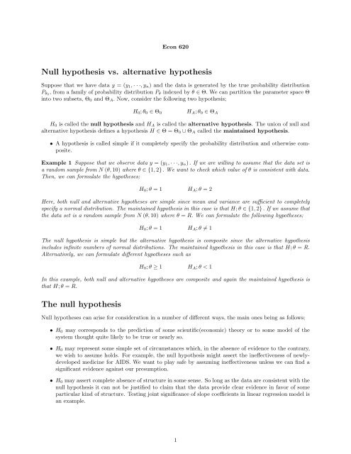
<strong>Null</strong> <strong>hypothesis</strong> <strong>vs</strong>. <strong>alternative</strong> <strong>hypothesis</strong><br />
Suppose that we have data y =(y 1 , ···,y n ) and the data is generated by the true probability distribution<br />
P θ0 , from a family of probability distribution P θ indexed by θ ∈ Θ. We can partition the parameter space Θ<br />
into two subsets, Θ 0 and Θ A . Now, consider the following two <strong>hypothesis</strong>;<br />
H 0 ; θ 0 ∈ Θ 0<br />
H A ; θ 0 ∈ Θ A<br />
H 0 is called the <strong>null</strong> <strong>hypothesis</strong> and H A is called the <strong>alternative</strong> <strong>hypothesis</strong>. <strong>The</strong> union of <strong>null</strong> and<br />
<strong>alternative</strong> <strong>hypothesis</strong> defines a <strong>hypothesis</strong> H ∈ Θ=Θ 0 ∪ Θ A called the maintained <strong>hypothesis</strong>.<br />
• A <strong>hypothesis</strong> is called simple if it completely specify the probability distribution and otherwise composite.<br />
Example 1 Suppose that we observe data y =(y 1 , ···,y n ) . If we are willing to assume that the data set is<br />
a random sample from N (θ, 10) where θ ∈{1, 2} . We want to check which value of θ is consistent with data.<br />
<strong>The</strong>n, we can formulate the hypotheses;<br />
H 0 ; θ =1 H A ; θ =2<br />
Here, both <strong>null</strong> and <strong>alternative</strong> hypotheses are simple since mean and variance are sufficient to completely<br />
specify a normal distribution. <strong>The</strong> maintained <strong>hypothesis</strong> in this case is that H; θ ∈{1, 2} . If we assume that<br />
the data set is a random sample from N (θ, 10) where θ = R. We can formulate the following hypotheses;<br />
H 0 ; θ =1<br />
H A ; θ ≠1<br />
<strong>The</strong> <strong>null</strong> <strong>hypothesis</strong> is simple but the <strong>alternative</strong> <strong>hypothesis</strong> is composite since the <strong>alternative</strong> <strong>hypothesis</strong><br />
includes infinite numbers of normal distributions. <strong>The</strong> maintained <strong>hypothesis</strong> in this case is that H; θ = R.<br />
Alternatively, we can formulate different hypotheses such as<br />
H 0 ; θ ≥ 1 H A ; θ
Type I and type II errors<br />
<strong>The</strong>re are four possible cases once we take an action in testing hypotheses - correctly accept the <strong>null</strong>, correctly<br />
reject the <strong>null</strong>, wrongly accept the <strong>null</strong> and wrongly reject the <strong>null</strong>. We don’t have any concern with the<br />
first two cases. A good test should avoid or minimize the possibilities of the last two cases.<br />
• Type I error is the probability that we reject the <strong>null</strong> <strong>hypothesis</strong> when it is true;<br />
α ≡ P [reject H 0 | H 0 is true]<br />
• Type II error is the probability that we do not reject the <strong>null</strong> <strong>hypothesis</strong> when it is not true;<br />
β ≡ P [do not reject H 0 | H A is true]<br />
• We call α,the probability that we reject the <strong>null</strong> <strong>hypothesis</strong> when it is true, size of the test<br />
• We call (1 − β) , the probability that we reject the <strong>null</strong> <strong>hypothesis</strong> when the <strong>alternative</strong> <strong>hypothesis</strong> is<br />
true, the power of the test.<br />
<strong>The</strong> ultimate goal in designing a test statistic is to minimize the size and maximize the power as much as<br />
possible. Unfortunately, it is quite easy to prove that we can not design a test which has both the minimum<br />
size and the maximum power. Here is an intuitive example why it is the case. Consider minimum size first.<br />
What is the test which has the minimum size? It is a test with which we always accept the <strong>null</strong> <strong>hypothesis</strong><br />
no matter what we observe from the data. Since we always accept the <strong>null</strong> <strong>hypothesis</strong>, the size of the test is<br />
0 which is the minimum possible size ; P [reject H 0 | H 0 is true] =0− note that we never reject. However,<br />
what is the power of this test? It is a pathetic test as far as power is concerned - power of the test is 0; 1−<br />
P [do not reject H 0 | H A is true] =1− 1=0. Now consider the opposite case - the test with which we<br />
always reject the <strong>null</strong> <strong>hypothesis</strong>. Power is great - it is 1, maximum possible power. But, the size of the test<br />
also is 1-again pathetic.<br />
We have to compromise between the two conflicting goals. Convention in testing procedure is to fix the<br />
size at a arbitrary prespecified level and search for a test which maximizes the power - even this is impossible<br />
in most cases.<br />
• Critical region of a test is the area where we commit the type I error.<br />
Test procedure and test statistic<br />
<strong>The</strong> next question naturally arising is that how we can actually test the hypotheses. An obvious answer<br />
is that the test, whatever it is, should be based on the observed data. <strong>The</strong> data set itself is too lousy to<br />
determine the plausibility of the <strong>null</strong> <strong>hypothesis</strong>. We need a kind of summary measure of the data, which<br />
should be handy but retain relevant information on the true data generating process.<br />
• Let t = t (y) be a function of the observations and let T = t (Y ) be the corresponding random variable.<br />
We call T a test statistic for the testing of H 0 if<br />
(i) the distribution of T when H 0 is true is knwon, at least approximately(asymptotically).<br />
(ii) the larger the value of t the stronger the evidence of departure from H 0 of the type<br />
it is required to test<br />
After getting the distribution of test statistic under the <strong>null</strong> <strong>hypothesis</strong>, we now need a decision rule to<br />
determine whether the <strong>null</strong> <strong>hypothesis</strong> is consistent with the observed data. For given observations y we can<br />
calculate t = t obs = t (y) , say, and identify a critical region for a given size of the test. If the value of the<br />
test statistic falls into the critical region, we reject the <strong>null</strong> <strong>hypothesis</strong>.<br />
To sum up the test procedure;<br />
1. Set up the <strong>null</strong> and <strong>alternative</strong> hypotheses<br />
2
2. Design a test statistic which has some good properties<br />
3. Find the distribution of test statistic under the <strong>null</strong> <strong>hypothesis</strong> - exact or asymptotic distribution<br />
4. Identify the critical region for the <strong>null</strong> distribution with a given size of the test<br />
5. Calculate the test statistic using the observed data<br />
6. Check whether or not the value of the test statistic falls into the critical region.<br />
3