
You also want an ePaper? Increase the reach of your titles
YUMPU automatically turns print PDFs into web optimized ePapers that Google loves.
Application Report<br />
SLOA058– November 2000<br />
A <strong>Single</strong>-<strong>Supply</strong> <strong>Op</strong>-<strong>Amp</strong> <strong>Circuit</strong> <strong>Collection</strong><br />
Bruce Carter<br />
<strong>Op</strong>-<strong>Amp</strong> Applications, High Performance Linear Products<br />
One of the biggest problems for designers of op-amp circuitry arises when the circuit must<br />
be operated from a single supply, rather than ±15 V. This application note provides<br />
working circuit examples.<br />
Contents<br />
1 Introduction ................................................................................................................................... 3<br />
1.1 Split <strong>Supply</strong> vs <strong>Single</strong> <strong>Supply</strong>.................................................................................................... 3<br />
1.2 Virtual Ground........................................................................................................................... 4<br />
1.3 AC-Coupling ............................................................................................................................. 4<br />
1.4 Combining <strong>Op</strong>-<strong>Amp</strong> Stages ...................................................................................................... 5<br />
1.5 Selecting Resistor and Capacitor Values .................................................................................. 5<br />
2 Basic <strong>Circuit</strong>s ................................................................................................................................ 5<br />
2.1 Gain.......................................................................................................................................... 5<br />
2.2 Attenuation ............................................................................................................................... 6<br />
2.3 Summing .................................................................................................................................. 9<br />
2.4 Difference <strong>Amp</strong>lifier .................................................................................................................. 9<br />
2.5 Simulated Inductor.................................................................................................................... 9<br />
2.6 Instrumentation <strong>Amp</strong>lifiers ...................................................................................................... 10<br />
3 Filter <strong>Circuit</strong>s ............................................................................................................................... 12<br />
3.1 <strong>Single</strong> Pole <strong>Circuit</strong>s................................................................................................................. 13<br />
3.1.1 Low Pass Filter <strong>Circuit</strong>s .............................................................................................................13<br />
3.1.2 High Pass Filter <strong>Circuit</strong>s.............................................................................................................13<br />
3.1.3 All-Pass Filter ............................................................................................................................14<br />
3.2 Double-Pole <strong>Circuit</strong>s ............................................................................................................... 15<br />
3.2.1 Sallen-Key.................................................................................................................................15<br />
3.2.2 Multiple Feedback (MFB)...........................................................................................................16<br />
3.2.3 Twin T .......................................................................................................................................17<br />
3.2.4 Fliege ........................................................................................................................................20<br />
3.2.5 Akerberg-Mossberg Filter ..........................................................................................................22<br />
3.2.6 BiQuad......................................................................................................................................24<br />
3.2.7 State Variable............................................................................................................................25<br />
4 References................................................................................................................................... 25<br />
Appendix A – Standard Resistor and Capacitor Values ................................................................. 26<br />
Figures<br />
1 Split <strong>Supply</strong> (L) vs <strong>Single</strong> <strong>Supply</strong> (R) <strong>Circuit</strong>s ..................................................................................3<br />
2 <strong>Single</strong>-<strong>Supply</strong> <strong>Op</strong>eration at Vcc/2....................................................................................................4<br />
3 AC-Coupled Gain Stages ................................................................................................................6<br />
4 Traditional Inverting Attenuation With an <strong>Op</strong> <strong>Amp</strong> ...........................................................................6<br />
5 Inverting Attenuation <strong>Circuit</strong> ............................................................................................................7<br />
6 Noninverting Attenuation .................................................................................................................8<br />
1
SLOA058<br />
7 Inverting Summing <strong>Circuit</strong> ...............................................................................................................9<br />
8 Subtracting <strong>Circuit</strong>...........................................................................................................................9<br />
9 Simulated Inductor <strong>Circuit</strong> .............................................................................................................10<br />
10 Basic Instrumentation-<strong>Amp</strong>lifier <strong>Circuit</strong>..........................................................................................11<br />
11 Simulated Instrumentation-<strong>Amp</strong>lifier <strong>Circuit</strong>...................................................................................11<br />
12 Instrumentation <strong>Circuit</strong> With Only Two <strong>Op</strong> <strong>Amp</strong>s...........................................................................12<br />
13 Low-Pass Filter <strong>Circuit</strong>s.................................................................................................................13<br />
14 High-Pass Filter <strong>Circuit</strong>s................................................................................................................14<br />
15 All-Pass Filter <strong>Circuit</strong>.....................................................................................................................14<br />
16 Sallen-Key Low- and High-Pass Filter Topologies.........................................................................16<br />
17 Multiple-Feedback Topologies.......................................................................................................17<br />
18 <strong>Single</strong> <strong>Op</strong>-<strong>Amp</strong> Twin-T Filter in Band-Pass Configuration .............................................................18<br />
19 <strong>Single</strong> <strong>Op</strong>-<strong>Amp</strong> Twin-T Filter in Notch Configuration .....................................................................18<br />
20 Dual-<strong>Op</strong>-<strong>Amp</strong> Twin-T Low-Pass Filter ...........................................................................................19<br />
21 Dual-<strong>Op</strong>-<strong>Amp</strong> Twin-T High-Pass Filter ..........................................................................................19<br />
22 Dual-<strong>Op</strong>-<strong>Amp</strong> Twin-T Notch Filter .................................................................................................20<br />
23 Low-Pass Fliege Filter...................................................................................................................20<br />
24 High-Pass Fliege Filter..................................................................................................................21<br />
25 Band-Pass Fliege Filter.................................................................................................................21<br />
26 Notch Fliege Filter.........................................................................................................................22<br />
27 Akerberg-Mossberg Low-Pass Filter .............................................................................................22<br />
28 Akerberg-Mossberg High-Pass Filter.............................................................................................23<br />
29 Akerberg-Mossberg Band-Pass Filter............................................................................................23<br />
30 Akerberg-Mossberg Notch Filter....................................................................................................24<br />
31 Biquad Low-Pass and Band-Pass Filter ........................................................................................24<br />
32 State-Variable Four-<strong>Op</strong>-<strong>Amp</strong> Topology .........................................................................................25<br />
Tables<br />
1 Normalization Factors .....................................................................................................................8<br />
2 A <strong>Single</strong>-<strong>Supply</strong> <strong>Op</strong>-<strong>Amp</strong> <strong>Circuit</strong> <strong>Collection</strong>
SLOA058<br />
1 Introduction<br />
There have been many excellent collections of op-amp circuits in the past, but all of them focus<br />
exclusively on split-supply circuits. Many times, the designer who has to operate a circuit from a<br />
single supply does not know how to do the conversion.<br />
<strong>Single</strong>-supply operation requires a little more care than split-supply circuits. The designer should<br />
read and understand this introductory material.<br />
1.1 Split <strong>Supply</strong> vs <strong>Single</strong> <strong>Supply</strong><br />
All op amps have two power pins. In most cases, they are labeled V CC+ and V CC- , but sometimes<br />
they are labeled V CC and GND. This is an attempt on the part of the data sheet author to<br />
categorize the part as a split-supply or single-supply part. However, it does not mean that the op<br />
amp has to be operated that way— it may or may not be able to operate from different voltage<br />
rails. Consult the data sheet for the op amp, especially the absolute maximum ratings and<br />
voltage-swing specifications, before operating at anything other than the recommended<br />
power-supply voltage(s).<br />
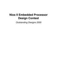
Most analog designers know how to use op amps with a split power supply. As shown in the left<br />
half of Figure 1, a split power supply consists of a positive supply and an equal and opposite<br />
negative supply. The most common values are ±15 V, but ±12 V and ±5 V are also used. The<br />
input and output voltages are referenced to ground, and swing both positive and negative to a<br />
limit of V OM± , the maximum peak-output voltage swing.<br />
A single-supply circuit (right side of Figure 1) connects the op-amp power pins to a positive<br />
voltage and ground. The positive voltage is connected to V CC+ , and ground is connected to V CCor<br />
GND. A virtual ground, halfway between the positive supply voltage and ground, is the<br />
reference for the input and output voltages. The voltage swings above and below this virtual<br />
ground to the limit of V OM± . Some newer op amps have different high- and low-voltage rails,<br />
which are specified in data sheets as V OH and V OL, respectively. It is important to note that there<br />
are very few cases when the designer has the liberty to reference the input and output to the<br />
virtual ground. In most cases, the input and output will be referenced to system ground, and the<br />
designer must use decoupling capacitors to isolate the dc potential of the virtual ground from the<br />
input and output (see section 1.3).<br />
+SUPPLY<br />
+SUPPLY<br />
-<br />
+<br />
HALF_SUPPLY<br />
-<br />
+<br />
-SUPPLY<br />
Figure 1.<br />
Split <strong>Supply</strong> (L) vs <strong>Single</strong> <strong>Supply</strong> (R) <strong>Circuit</strong>s<br />
A common value for single supplies is 5 V, but voltage rails are getting lower, with 3 V and even<br />
lower voltages becoming common. Because of this, single-supply op amps are often rail-to-rail<br />
devices, which avoids losing dynamic range. Rail-to-rail may or may not apply to both the input<br />
and output stages. Be aware that even though a device might be specified as rail-to-rail, some<br />
A <strong>Single</strong>-<strong>Supply</strong> <strong>Op</strong>-<strong>Amp</strong> <strong>Circuit</strong> <strong>Collection</strong> 3
SLOA058<br />
specifications can degrade close to the rails. Be sure to consult the data sheet for complete<br />
specifications on both the inputs and outputs. It is the designer’s obligation to ensure that the<br />
voltage rails of the op amp do not degrade the system specifications.<br />
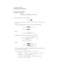
1.2 Virtual Ground<br />
<strong>Single</strong>-supply operation requires the generation of a virtual ground, usually at a voltage equal to<br />
Vcc/2. The circuit in Figure 2 can be used to generate Vcc/2, but its performance deteriorates at<br />
low frequencies.<br />
+Vcc<br />
+Vcc<br />
R1<br />
100 kW<br />
R2<br />
100 kW<br />
C1<br />
0.1 mF<br />
-<br />
+<br />
Vcc/2<br />
Figure 2.<br />
<strong>Single</strong>-<strong>Supply</strong> <strong>Op</strong>eration at VCC/2<br />
R1 and R2 are equal values, selected with power consumption vs allowable noise in mind.<br />
Capacitor C1 forms a low-pass filter to eliminate conducted noise on the voltage rail. Some<br />
applications can omit the buffer op amp.<br />
In what follows, there are a few circuits in which a virtual ground has to be introduced with two<br />
resistors within the circuit because one virtual ground is not suitable. In these instances, the<br />
resistors should be 100 kW or greater; when such a case arises, values are indicated on the<br />
schematic.<br />
1.3 AC-Coupling<br />
A virtual ground is at a dc level above system ground; in effect, a small, local-ground system has<br />
been created within the op-amp stage. However, there is a potential problem: the input source<br />
and output load are probably referenced to system ground, and if the op-amp stage is connected<br />
to a source that is referenced to ground instead of virtual ground, there will be an unacceptable<br />
dc offset. If this happens, the op amp becomes unable to operate on the input signal, because it<br />
must then process signals at and below its input and output rails.<br />
The solution is to ac-couple the signals to and from the op-amp stage. In this way, the input and<br />
output devices can be referenced to ground, and the op-amp circuitry can be referenced to a<br />
virtual ground.<br />
When more than one op-amp stage is used, interstage decoupling capacitors might become<br />
unnecessary if all of the following conditions are met:<br />
• The first stage is referenced to virtual ground.<br />
• The second stage is referenced to virtual ground.<br />
4 A <strong>Single</strong>-<strong>Supply</strong> <strong>Op</strong>-<strong>Amp</strong> <strong>Circuit</strong> <strong>Collection</strong>
• There is no gain in either stage. Any dc offset in either stage is multiplied by the gain in<br />
both, and probably takes the circuit out of its normal operating range.<br />
SLOA058<br />
If there is any doubt, assemble a prototype including ac-coupling capacitors, then remove them<br />
one at a time. Unless the input or output are referenced to virtual ground, there must be an<br />
input-decoupling capacitor to decouple the source and an output-decoupling capacitor to<br />
decouple the load. A good troubleshooting technique for ac circuits is to terminate the input and<br />
output, then check the dc voltage at all op-amp inverting and noninverting inputs and at the<br />
op-amp outputs. All dc voltages should be very close to the virtual-ground value. If they are not,<br />
decoupling capacitors are mandatory in the previous stage (or something is wrong with the<br />
circuit).<br />
1.4 Combining <strong>Op</strong>-<strong>Amp</strong> Stages<br />
Combining op-amp stages to save money and board space is possible in some cases, but it<br />
often leads to unavoidable interactions between filter response characteristics, offset voltages,<br />
noise, and other circuit characteristics. The designer should always begin by prototyping<br />
separate gain, offset, and filter stages, then combine them if possible after each individual circuit<br />
function has been verified. Unless otherwise specified, filter circuits included in this document<br />
are unity gain.<br />
1.5 Selecting Resistor and Capacitor Values<br />
The designer who is new to analog design often wonders how to select component values.<br />
Should resistors be in the 1-Ω decade or the 1-MΩ decade Resistor values in the 1-kΩ to<br />
100-kΩ range are good for general-purpose applications. High-speed applications usually use<br />
resistors in the 100-Ω to 1-kΩ decade, and they consume more power. Portable applications<br />
usually use resistors in the 1-MΩ or even 10-MΩ decade, and they are more prone to noise.<br />
Basic formulas for selecting resistor and capacitor values for tuned circuits are given in the<br />
various figures. For filter applications, resistors should be chosen from 1% E-96 values (see<br />
Appendix A). Once the resistor decade range has been selected, choose standard E-12 value<br />
capacitors. Some tuned circuits may require E-24 values, but they should be avoided where<br />
possible. Capacitors with only 5% tolerance should be avoided in critical tuned circuits— use 1%<br />
instead.<br />
2 Basic <strong>Circuit</strong>s<br />
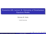
2.1 Gain<br />
Gain stages come in two basic varieties: inverting and noninverting. The ac-coupled version is<br />
shown in Figure 3. For ac circuits, inversion means an ac-phase shift of 180°. These circuits<br />
work by taking advantage of the coupling capacitor, CIN, to prevent the circuit from having dc<br />
gain. They have ac gain only. If CIN is omitted in a dc system, dc gain must be taken into<br />
account.<br />
It is very important not to violate the bandwidth limit of the op amp at the highest frequency seen<br />
by the circuit. Practical circuits can include gains of 100 (40 dB), but higher gains could cause<br />
the circuit to oscillate unless special care is taken during PC board layout. It is better to cascade<br />
two or more equal-gain stages than to attempt high gain in a single stage.<br />
A <strong>Single</strong>-<strong>Supply</strong> <strong>Op</strong>-<strong>Amp</strong> <strong>Circuit</strong> <strong>Collection</strong> 5
SLOA058<br />
R2<br />
INVERTING<br />
Gain = – R2/R1<br />
R3 = R1||R2<br />
for minimum error due<br />
to input bias current<br />
Vin<br />
Cin<br />
R1<br />
+Vcc<br />
-<br />
+<br />
Vout<br />
R3<br />
Vcc/2<br />
+Vcc<br />
NONINVERTING<br />
Gain = 1 + R2/R1<br />
Input Impedance = R1||R2<br />
Vin<br />
Cin<br />
+<br />
-<br />
Vout<br />
for minimum error due<br />
to input bias current<br />
R2<br />
R1<br />
Vcc/2<br />
Figure 3.<br />
AC-Coupled Gain Stages<br />
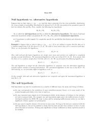
2.2 Attenuation<br />
The traditional way of doing inverting attenuation with an op-amp circuit is shown in Figure 4, in<br />
R2<br />
INVERTING<br />
Gain = – R2/R1<br />
R3 = R1||R2<br />
for minimum error due<br />
to input bias current<br />
Vin<br />
Cin<br />
R1<br />
+Vcc<br />
-<br />
+<br />
Vout<br />
R3<br />
Vcc/2<br />
Figure 4.<br />
Traditional Inverting Attenuation With an <strong>Op</strong> <strong>Amp</strong><br />
which R2 < R1. This method is not recommended, because many op amps are unstable at gains<br />
of less than unity. The correct way to construct an attenuation circuit 1 is shown in Figure 5.<br />
1 This circuit is taken from the design notes of William Ezell<br />
6 A <strong>Single</strong>-<strong>Supply</strong> <strong>Op</strong>-<strong>Amp</strong> <strong>Circuit</strong> <strong>Collection</strong>
SLOA058<br />
Rf 2<br />
INVERTING<br />
Component values<br />
normalized to unity Cin RinA 1 RinB 1<br />
Vin<br />
R3<br />
+Vcc<br />
-<br />
+<br />
Vout<br />
Vcc/2<br />
Figure 5.<br />
Inverting Attenuation <strong>Circuit</strong><br />
A set of normalized values of the resistor R3 for various levels of attenuation is shown in<br />
Table 1. For nontablated attenuation values, the resistance is:<br />
R<br />
3<br />
=<br />
V<br />
2 − 2<br />
O<br />
V<br />
( V V )<br />
O<br />
IN<br />
IN<br />
To work with normalized values, do the following:<br />
• Select a base-value of resistance, usually between 1 kW and 100 kW for Rf and Rin.<br />
• Divide Rin in two for RinA and RinB.<br />
• Multiply the base value for Rf and Rin by 1 or 2, as shown in Figure 5.<br />
• Look up the normalization factor for R3 in the table below, and multiply it by the base-value<br />
of resistance.<br />
For example, if Rf is 20 kΩ, RinA and RinB are each 10 kΩ, and a 3-dB attenuator would use a<br />
12.1-kΩ resistor.<br />
A <strong>Single</strong>-<strong>Supply</strong> <strong>Op</strong>-<strong>Amp</strong> <strong>Circuit</strong> <strong>Collection</strong> 7
SLOA058<br />
Table 1.<br />
Normalization Factors<br />
DB Pad Vout/Vin R3<br />
0 1.0000 ∞<br />
0.5 0.9441 8.4383<br />
1 0.8913 4.0977<br />
2 0.7943 0.9311<br />
2 0.7079 1.2120<br />
3.01 0.7071 1.2071<br />
3.52 0.6667 1.000<br />
4 0.6310 0.8549<br />
5 0.5623 0.6424<br />
6 0.5012 0.5024<br />
6.02 0.5000 0.5000<br />
7 0.4467 0.4036<br />
8 0.3981 0.3307<br />
9 0.3548 0.2750<br />
9.54 0.3333 0.2500<br />
10 0.3162 0.2312<br />
12 0.2512 0.1677<br />
12.04 0.2500 0.1667<br />
13.98 0.2000 0.1250<br />
15 0.1778 0.1081<br />
15.56 0.1667 0.1000<br />
16.90 0.1429 0.08333<br />
18 0.1259 0.07201<br />
18.06 0.1250 0.07143<br />
19.08 0.1111 0.06250<br />
20 0.1000 0.05556<br />
25 0.0562 0.02979<br />
30 0.0316 0.01633<br />
40 0.0100 0.005051<br />
50 0.0032 0.001586<br />
60 0.0010 0.0005005<br />
Noninverting attenuation can be performed with a voltage divider and a noninverting buffer as<br />
shown in Figure 6.<br />
NONINVERTING<br />
+Vcc<br />
Component values<br />
normalized to unity<br />
Vin<br />
Cin<br />
R1<br />
R2<br />
+<br />
-<br />
Vout<br />
Vcc/2<br />
Figure 6.<br />
Noninverting Attenuation<br />
8 A <strong>Single</strong>-<strong>Supply</strong> <strong>Op</strong>-<strong>Amp</strong> <strong>Circuit</strong> <strong>Collection</strong>
SLOA058<br />
2.3 Summing<br />
An inverting summing circuit (Figure 7) is the basis of an audio mixer. A single-supply voltage is<br />
seldom used for real audio mixers. Designers will often push an op amp up to, and sometimes<br />
beyond, its recommended voltage rails to increase dynamic range.<br />
Noninverting summing circuits are possible, but not recommended. The source impedance<br />
becomes part of the gain calculation.<br />
INVERTING<br />
Vout = – R2(Vin1/R1 + Vin2/R2 +<br />
Vin3/R3)<br />
= R1A||R1B||R1C||R2<br />
for minimum error due<br />
to input bias current<br />
Vin1<br />
Vin2<br />
Vin3<br />
Cin1<br />
Cin2<br />
CIin3<br />
R1A<br />
R1B<br />
R1C<br />
+Vcc<br />
-<br />
+<br />
R2<br />
Vout<br />
R3<br />
Vcc/2<br />
Figure 7.<br />
Inverting Summing <strong>Circuit</strong><br />
2.4 Difference <strong>Amp</strong>lifier<br />
Just as there are summing circuits, there are also subtracting circuits (Figure 8). A common<br />
application is to eliminate the vocal track (recorded at equal levels in both channels) from stereo<br />
recordings.<br />
R2<br />
For R1 = R3 and R2 = R4:<br />
Vout = (R2/R1)(Vin2 – Vin1)<br />
R1||R2 = R3||R4<br />
for minimum error due<br />
to input bias current<br />
Vin1<br />
Vin2<br />
Cin1<br />
Cin2<br />
R1<br />
R3<br />
+Vcc<br />
-<br />
+<br />
Vout<br />
R4<br />
Vcc/2<br />
Figure 8.<br />
Subtracting <strong>Circuit</strong><br />
2.5 Simulated Inductor<br />
The circuit in Figure 9 reverses the operation of a capacitor, thus making a simulated inductor.<br />
An inductor resists any change in its current, so when a dc voltage is applied to an inductance,<br />
the current rises slowly, and the voltage falls as the external resistance becomes more<br />
significant.<br />
A <strong>Single</strong>-<strong>Supply</strong> <strong>Op</strong>-<strong>Amp</strong> <strong>Circuit</strong> <strong>Collection</strong> 9
SLOA058<br />
+Vcc<br />
L = R1*R2*C1<br />
Vin1<br />
C1<br />
R2<br />
+<br />
-<br />
Vout<br />
Vcc/2<br />
R1<br />
Figure 9.<br />
Simulated Inductor <strong>Circuit</strong><br />
An inductor passes low frequencies more readily than high frequencies, the opposite of a<br />
capacitor. An ideal inductor has zero resistance. It passes dc without limitation, but it has infinite<br />
impedance at infinite frequency.<br />
If a dc voltage is suddenly applied to the inverting input through resistor R1, the op amp ignores<br />
the sudden load because the change is also coupled directly to the noninverting input via C1.<br />
The op amp represents high impedance, just as an inductor does.<br />
As C1 charges through R2, the voltage across R2 falls, so the op-amp draws current from the<br />
input through R1. This continues as the capacitor charges, and eventually the op-amp has an<br />
input and output close to virtual ground (Vcc/2).<br />
When C1 is fully charged, resistor R1 limits the current flow, and this appears as a series<br />
resistance within the simulated inductor. This series resistance limits the Q of the inductor. Real<br />
inductors generally have much less resistance than the simulated variety.<br />
There are some limitations of a simulated inductor:<br />
• One end of the inductor is connected to virtual ground.<br />
• The simulated inductor cannot be made with high Q, due to the series resistor R1.<br />
• It does not have the same energy storage as a real inductor. The collapse of the magnetic<br />
field in a real inductor causes large voltage spikes of opposite polarity. The simulated<br />
inductor is limited to the voltage swing of the op amp, so the flyback pulse is limited to the<br />
voltage swing.<br />
2.6 Instrumentation <strong>Amp</strong>lifiers<br />
Instrumentation amplifiers are used whenever dc gain is needed on a low-level signal that would<br />
be loaded by conventional differential-amplifier topologies. Instrumentation amplifiers take<br />
advantage of the high input impedance of noninverting op-amp inputs.<br />
The basic instrumentation amplifier topology is shown in Figure 10.<br />
10 A <strong>Single</strong>-<strong>Supply</strong> <strong>Op</strong>-<strong>Amp</strong> <strong>Circuit</strong> <strong>Collection</strong>
SLOA058<br />
+Vcc<br />
Vin-<br />
+<br />
-<br />
R1<br />
R2<br />
ASSUMES Vin- AND Vin+<br />
REFERENCED TO Vcc/2<br />
R5<br />
+Vcc<br />
R1 = R3 (matched)<br />
R2 = R4 (matched)<br />
R5 = R6<br />
Gain = R2/R1 (1 + 2R5/R7)<br />
+Vcc<br />
R7<br />
-<br />
+<br />
Vout<br />
R6<br />
-<br />
R3<br />
Vin+<br />
+<br />
R4<br />
Vcc/2<br />
Figure 10. Basic Instrumentation-<strong>Amp</strong>lifier <strong>Circuit</strong><br />
This circuit, and the other instrumentation amplifier topologies presented here, assume that the<br />
inputs are already referenced to half-supply. This is the case with strain gauges that are<br />
operated from Vcc. The basic disadvantage of this circuit is that it requires matched resistors;<br />
otherwise, it would suffer from poor CMRR (see for example, <strong>Op</strong> <strong>Amp</strong>s for Everyone [3] ).<br />
The circuit in Figure 10 can be simplified by eliminating three resistors, as shown in Figure 11.<br />
+Vcc<br />
Vin-<br />
+<br />
-<br />
R1<br />
R2<br />
ASSUMES Vin- AND Vin+<br />
REFERENCED TO Vcc/2<br />
+Vcc<br />
R1 = R3 (matched)<br />
R2 = R4 (matched)<br />
Gain = R2/R1<br />
+Vcc<br />
-<br />
+<br />
Vout<br />
-<br />
R3<br />
Vin+<br />
+<br />
R4<br />
Vcc/2<br />
Figure 11. Modified Instrumentation-<strong>Amp</strong>lifier <strong>Circuit</strong><br />
A <strong>Single</strong>-<strong>Supply</strong> <strong>Op</strong>-<strong>Amp</strong> <strong>Circuit</strong> <strong>Collection</strong> 11
SLOA058<br />
Here, the gain is easier to calculate, but a disadvantage is that now two resistors must be<br />
changed instead of one, and they must be matched resistors. Another disadvantage is that the<br />
first stage(s) cannot be used for gain.<br />
An instrumentation amplifier can also be made from two op amps; this is shown in Figure 12.<br />
R1<br />
R2<br />
R3<br />
R4<br />
ASSUMES Vin- AND Vin+<br />
REFERENCED TO Vcc/2<br />
Vcc/2<br />
+Vcc<br />
+Vcc<br />
R1 = R4 (matched)<br />
R2 = R3 (matched)<br />
Gain = 1 + R1/R2<br />
-<br />
+<br />
-<br />
+<br />
Vout<br />
Vin -<br />
Vin+<br />
Figure 12. Instrumentation <strong>Circuit</strong> With Only Two <strong>Op</strong> <strong>Amp</strong>s<br />
However, this topology is not recommended because the first op amp is operated at less than<br />
unity gain, so it may be unstable. Furthermore, the signal from Vin- has more propagation delay<br />
than Vin+.<br />
3 Filter <strong>Circuit</strong>s<br />
This section is devoted to op-amp active filters. In many cases, it is necessary to block dc<br />
voltage from the virtual ground of the op-amp stage by adding a capacitor to the input of the<br />
circuit. This capacitor forms a high-pass filter with the input so, in a sense, all these circuits have<br />
a high-pass characteristic. The designer must insure that the input capacitor is at least 100 times<br />
the value of the other capacitors in the circuit, so that the high-pass characteristic does not come<br />
into play at the frequencies of interest in the circuit. For filter circuits with gain, 1000 times might<br />
be better. If the input voltage already contains a Vcc/2 offset, the capacitor can be omitted.<br />
These circuits will have a half-supply dc offset at their output. If the circuit is the last stage in the<br />
system, an output-coupling capacitor may also be required.<br />
There are trade-offs involved in filter design. The most desirable situation is to implement a filter<br />
with a single op amp. Ideally, the filter would be simple to implement, and the designer would<br />
have complete control over:<br />
• The filter corner / center frequency<br />
• The gain of the filter circuit<br />
• The Q of band-pass and notch filters, or style of low-pass and high-pass filter (Butterworth,<br />
Chebyshev, or Bessell).<br />
12 A <strong>Single</strong>-<strong>Supply</strong> <strong>Op</strong>-<strong>Amp</strong> <strong>Circuit</strong> <strong>Collection</strong>
SLOA058<br />
Unfortunately, such is not the case— complete control over the filter is seldom possible with a<br />
single op amp. If control is possible, it frequently involves complex interactions between passive<br />
components, and this means complex mathematical calculations that intimidate many designers.<br />
More control usually means more op amps, which may be acceptable in designs that will not be<br />
produced in large volumes, or that may be subject to several changes before the design is<br />
finalized. If the designer needs to implement a filter with as few components as possible, there<br />
will be no choice but to resort to traditional filter-design techniques and perform the necessary<br />
calculations.<br />
3.1 <strong>Single</strong> Pole <strong>Circuit</strong>s<br />
<strong>Single</strong>-pole circuits are the simplest filter circuits. They have a roll off of 20 dB per decade.<br />
3.1.1 Low Pass Filter <strong>Circuit</strong>s<br />
Typical low-pass filter circuits are shown in Figure 13.<br />
INVERTING<br />
R2<br />
C1<br />
Fo = 1/(2pR2C1)<br />
Gain = – R2/R1<br />
+Vcc<br />
Vin<br />
Cin<br />
R1<br />
Vcc/2<br />
-<br />
+<br />
Vout<br />
+Vcc<br />
Vin<br />
Cin<br />
R1<br />
+<br />
-<br />
Vout<br />
NONINVERTING<br />
Fo = 1/(2pR1C1)<br />
Gain = 1 + R3/R2<br />
C1<br />
R2<br />
R3<br />
Vcc/2<br />
Figure 13. Low-Pass Filter <strong>Circuit</strong>s<br />
3.1.2 High Pass Filter <strong>Circuit</strong>s<br />
Typical high-pass filter circuits are shown in Figure 14.<br />
A <strong>Single</strong>-<strong>Supply</strong> <strong>Op</strong>-<strong>Amp</strong> <strong>Circuit</strong> <strong>Collection</strong> 13
SLOA058<br />
+Vcc<br />
C1<br />
NONINVERTING<br />
Gain = 1<br />
Fo = 1/(2pR1C1)<br />
Vin<br />
R1<br />
Vcc/2<br />
+<br />
-<br />
Vout<br />
+Vcc<br />
NONINVERTING<br />
Vin<br />
C1<br />
+<br />
-<br />
Vout<br />
Fo = 1/(2pR1C1)<br />
Gain = 1 + R3/R2<br />
R1<br />
R2<br />
R3<br />
Vcc/2<br />
Figure 14. High-Pass Filter <strong>Circuit</strong>s<br />
3.1.3 All-Pass Filter<br />
The all-pass filter passes all frequencies at the same gain. It is used to change the phase of the<br />
signal, and it can also be used as a phase-correction circuit. The circuit shown in Figure 15 has<br />
a 90°phase shift at F(90). At dc, the phase shift is 0°, and at high frequencies it is 180°.<br />
+Vcc<br />
C1<br />
R1 = R2 = R3 = R<br />
F(90) = 1/(2pR*C1)<br />
Vin1<br />
R2<br />
+<br />
-<br />
Vout<br />
Vcc/2<br />
R1<br />
R3<br />
Figure 15. All-Pass Filter <strong>Circuit</strong><br />
14 A <strong>Single</strong>-<strong>Supply</strong> <strong>Op</strong>-<strong>Amp</strong> <strong>Circuit</strong> <strong>Collection</strong>
SLOA058<br />
3.2 Double-Pole <strong>Circuit</strong>s<br />
Double-pole op-amp circuit topologies are sometimes named after their inventor. Several<br />
implementations or topologies exist. Some double-pole circuit topologies are available in a<br />
low-pass, high-pass, band-pass, and notch configuration. Others are not. Not all topologies and<br />
implementations are given here: only the ones that are easy to implement and tune.<br />
Double-pole or second-order filters have a 40-dB-per-decade roll-off.<br />
Commonly the same component(s) adjust the Q for the band-pass and notch versions of the<br />
topology, and they change the filter from Butterworth to Chebyshev, etc. for low-pass and highpass<br />
versions of the topology. Be aware that the corner frequency calculation is only valid for the<br />
Butterworth versions of the topologies. Chebyshev and Bessell modify it slightly.<br />
When band-pass and notch filter circuits are shown, they are high-Q (single frequency) types. To<br />
implement a wider band-pass or notch (band-reject) filter, cascade low-pass and high-pass<br />
stages. The pass characteristics should overlap for a band-pass and not overlap for a<br />
band-reject filter.<br />
Inverse Chebyshev and Elliptic filters are not shown. These are beyond the scope of a circuit<br />
collection note.<br />
Not all filter topologies produce ideal results— the final attenuation in the rejection band, for<br />
example, is greater in the multiple-feedback filter configuration than it is in the Sallen-Key filter.<br />
These fine points are beyond the scope of an op-amp circuit collection. Consult a textbook on<br />
filter design for the merits and drawbacks of each of these topologies. Unless the application is<br />
particularly critical, all the circuits shown here should produce acceptable results.<br />
3.2.1 Sallen-Key<br />
The Sallen-Key topology is one of the most widely-known and popular second-order topologies.<br />
It is low cost, requiring only a single op amp and four passive components to accomplish the<br />
tuning. Tuning is easy, but changing the style of filter from Butterworth to Chebyshev is not. The<br />
designer is encouraged to read references [1] and [2] for a detailed description of this topology.<br />
The circuits shown are unity gain— changing the gain of a Sallen-Key circuit also changes the<br />
filter tuning and the style. It is easiest to implement a Sallen-Key filter as a unity gain<br />
Butterworth.<br />
A <strong>Single</strong>-<strong>Supply</strong> <strong>Op</strong>-<strong>Amp</strong> <strong>Circuit</strong> <strong>Collection</strong> 15
SLOA058<br />
+Vcc<br />
LOW PASS<br />
Unity Gain<br />
Butterworth<br />
R3 = R4 (HIGH)<br />
R1 = R2<br />
C1 = 2C2<br />
Fo = 2 / (4pR1C2)<br />
Vin<br />
Cin<br />
R4<br />
R3<br />
R1<br />
R2<br />
C2<br />
C1<br />
+Vcc<br />
+<br />
-<br />
Vout<br />
HIGH PASS<br />
R1<br />
+Vcc<br />
Unity Gain<br />
Butterworth<br />
C1 = C2<br />
R1 = R<br />
R = 2R1<br />
Fo = 2 / (4pR1C1)<br />
Vin<br />
C1<br />
C2<br />
R2<br />
+<br />
-<br />
Vout<br />
Vcc/2<br />
Figure 16. Sallen-Key Low- and High-Pass Filter Topologies<br />
3.2.2 Multiple Feedback (MFB)<br />
MFB topology is very versatile, low cost, and easy to implement. Unfortunately, calculations are<br />
somewhat complex, and certainly beyond the scope of this circuit collection. The designer is<br />
encouraged to read reference [1] for a detailed description of the MFB topology. If all that is<br />
needed is a unity gain Butterworth, then these circuits will provide a close approximation.<br />
16 A <strong>Single</strong>-<strong>Supply</strong> <strong>Op</strong>-<strong>Amp</strong> <strong>Circuit</strong> <strong>Collection</strong>
SLOA058<br />
LOW PASS<br />
Unity Gain Butterworth<br />
Fo = 1/(2pRC)<br />
R1 = R2 = R/ 2<br />
R3 = R/(2 2)<br />
C1 = C<br />
C2 = 4C<br />
Vin<br />
Cin R1<br />
C2<br />
Vcc/2<br />
R2<br />
R3<br />
C1<br />
+Vcc<br />
-<br />
+<br />
Vout<br />
HIGH PASS<br />
+Vcc<br />
Unity Gain Butterworth<br />
Fo = 1/(2pRC)<br />
R1 = 0.47R<br />
R2 = 2.1R<br />
C1 = C2 = C3 = C<br />
Vin<br />
C1<br />
R1<br />
C2<br />
C3<br />
R2<br />
-<br />
+<br />
Vout<br />
Vcc/2<br />
BAND PASS<br />
C1<br />
R3<br />
+Vcc<br />
Gain = 2.3 dB<br />
Fo = 1/(2.32pRC)<br />
R1 = 10R<br />
R2 = 0.001R<br />
R3 = 100R<br />
C1 = 10C<br />
C2 = C<br />
Vin<br />
Cin R1<br />
R2<br />
Vcc/2<br />
C2<br />
-<br />
+<br />
Vout<br />
Figure 17. Multiple-Feedback Topologies<br />
3.2.3 Twin T<br />
The twin-T topology uses either one or two op amps. It is based on a passive (RC) topology that<br />
uses three resistors and three capacitors. Matching these six passive components is critical;<br />
fortunately, it is also easy. The entire network can be constructed from a single value of<br />
resistance and a single value of capacitance, running them in parallel to create R3 and C3 in the<br />
twin-T schematics shown in Figure. Components from the same batch are likely to have very<br />
similar characteristics.<br />
A <strong>Single</strong>-<strong>Supply</strong> <strong>Op</strong>-<strong>Amp</strong> <strong>Circuit</strong> <strong>Collection</strong> 17
SLOA058<br />
3.2.3.1 <strong>Single</strong> <strong>Op</strong>-<strong>Amp</strong> Implementations<br />
R1<br />
R2<br />
C3<br />
Vcc/2<br />
BAND PASS<br />
R1 = R2 = R<br />
C1 = C2 = C<br />
R3 = R/2<br />
C3 = 2C<br />
Fo = 1/(2pRC)<br />
Vin<br />
Gain controlled by R4 and R5<br />
R4 > 100 * R5<br />
Q hard to control; need mismatched<br />
Resistors; also affects gain<br />
Cin<br />
R4<br />
R5<br />
C1<br />
+Vcc<br />
-<br />
+<br />
R3<br />
C2<br />
Vout<br />
Vcc/2<br />
Figure 18. <strong>Single</strong> <strong>Op</strong>-<strong>Amp</strong> Twin-T Filter in Band-Pass Configuration<br />
The bandpass circuit will oscillate if the components are matched too closely. It is best to<br />
de-tune it slightly, by selecting the resistor to virtual ground to be one E-96 1% resistor value off,<br />
for instance.<br />
+Vcc<br />
NOTCH<br />
R4<br />
C1<br />
C2<br />
+Vcc<br />
C1 = C2 = C<br />
C3 = 2C<br />
R1 = R2 = R<br />
R3 = R/2<br />
Fo = 1/(2pRC)<br />
Vin<br />
Cin<br />
Vcc/2<br />
R3<br />
C3<br />
+<br />
-<br />
Vout<br />
R4 = R5: HIGH<br />
The only control over Q<br />
is by mismatching R3<br />
R5<br />
R1<br />
R2<br />
Figure 19. <strong>Single</strong> <strong>Op</strong>-<strong>Amp</strong> Twin-T Filter in Notch Configuration<br />
18 A <strong>Single</strong>-<strong>Supply</strong> <strong>Op</strong>-<strong>Amp</strong> <strong>Circuit</strong> <strong>Collection</strong>
SLOA058<br />
3.2.3.2 Dual-<strong>Op</strong>-<strong>Amp</strong> Implementations<br />
Typical dual op-amp implementations are shown in Figures 20 to 22<br />
LOW PASS<br />
R1 = R2 = R<br />
C1 = C2 = C<br />
R3 = R/2<br />
C3 = 2C<br />
Fo = 1/(2pRC)<br />
Vin<br />
Cin<br />
+Vcc<br />
R6<br />
R1<br />
R2<br />
+Vcc<br />
-<br />
+<br />
Vout<br />
Unity Gain<br />
R4 < R5/2 Chebyshev<br />
R4 = R5/2 Butterworth<br />
R4 > R5/2 Bessel<br />
R7<br />
C3<br />
+Vcc<br />
R6 = R7: HIGH<br />
Vcc/2<br />
C1<br />
R3<br />
C2<br />
-<br />
+<br />
R4<br />
R5<br />
Vcc/2<br />
Figure 20. Dual-<strong>Op</strong>-<strong>Amp</strong> Twin-T Low-Pass Filter<br />
+Vcc<br />
HIGH PASS<br />
R1 = R2 = R<br />
C1 = C2 = C<br />
R3 = R/2<br />
C3 = 2C<br />
Fo = 1/(2pRC)<br />
Vcc/2<br />
R1<br />
C3<br />
R2<br />
-<br />
+<br />
Vout<br />
Unity Gain<br />
R4 < R5/2 Chebyshev<br />
R4 = R5/2 Butterworth<br />
R4 > R5/2 Bessel<br />
Vin<br />
C1<br />
R3<br />
C2<br />
+Vcc<br />
-<br />
+<br />
R4<br />
R5<br />
Vcc/2<br />
Figure 21. Dual-<strong>Op</strong>-<strong>Amp</strong> Twin-T High-Pass Filter<br />
A <strong>Single</strong>-<strong>Supply</strong> <strong>Op</strong>-<strong>Amp</strong> <strong>Circuit</strong> <strong>Collection</strong> 19
SLOA058<br />
+Vcc<br />
+Vcc<br />
NOTCH<br />
R6<br />
R1 = R2 = R<br />
C1 = C2 = C<br />
R3 = R/2<br />
C3 = 2C<br />
Fo = 1/(2pRC)<br />
R6 = R7 > 20*R<br />
Vin<br />
CIN<br />
R7<br />
R1<br />
C3<br />
R2<br />
-<br />
+<br />
Vout<br />
Q controlled by<br />
ratio of R5 and R4<br />
R4 = 0.05*R5: high Q<br />
R4 = 0.5*R5 low: Q<br />
C1<br />
R3<br />
C2<br />
+Vcc<br />
-<br />
R4<br />
+<br />
R5<br />
Vcc/2<br />
Figure 22. Dual-<strong>Op</strong>-<strong>Amp</strong> Twin-T Notch Filter<br />
3.2.4 Fliege<br />
Fliege is a two-op-amp topology (Figures 23–26), and therefore more expensive than one-opamp<br />
topologies. There is good control over the tuning and the Q and style of filter. The gain is<br />
fixed at two for low-pass, high-pass, and band-pass filters, and unity for notch.<br />
+Vcc<br />
LOW PASS<br />
R2 = R3 = R<br />
C1 = C2 = C<br />
R4 = R5, not critical<br />
Fo = 1/(2pRC)<br />
Gain fixed at 2<br />
R1 = R/ 2 Butterworth<br />
R1 > R/ 2 Chebyshev<br />
R1 < R/ 2 Bessel<br />
Vin<br />
Cin<br />
R2<br />
R1<br />
C1<br />
R3<br />
+Vcc<br />
-<br />
+<br />
+<br />
-<br />
R4<br />
C2<br />
Vout<br />
R5<br />
Vcc/2<br />
Figure 23. Low-Pass Fliege Filter<br />
20 A <strong>Single</strong>-<strong>Supply</strong> <strong>Op</strong>-<strong>Amp</strong> <strong>Circuit</strong> <strong>Collection</strong>
SLOA058<br />
+Vcc<br />
HIGH PASS<br />
R2 = R3 = R<br />
C1 = C2 = C<br />
R4 = R5, not critical<br />
Fo = 1/(2pRC)<br />
Gain fixed at 2<br />
R1 = R/ 2 Butterworth<br />
R1 > R/ 2 Chebyshev<br />
R1 < R/ 2 Bessel<br />
Vin<br />
C1<br />
R1<br />
Vcc/2<br />
R2<br />
C2<br />
+Vcc<br />
-<br />
+<br />
+<br />
-<br />
R3<br />
R4<br />
Vout<br />
R5<br />
Vcc/2<br />
Figure 24. High-Pass Fliege Filter<br />
+Vcc<br />
BAND PASS<br />
Vin<br />
Cin<br />
R1<br />
+<br />
-<br />
Vout<br />
Gain fixed at 2<br />
R1 controls Q<br />
low R1 => low Q<br />
high R1 => high Q<br />
R1 should be > R/5<br />
C1<br />
Vcc/2<br />
R2<br />
C2<br />
+Vcc<br />
R3<br />
R2 = R3 = R<br />
C1 = C2 = C<br />
R4 = R5, not critical<br />
Fo = 1/(2pRC)<br />
-<br />
+<br />
R4<br />
R5<br />
Vcc/2<br />
Figure 25. Band-Pass Fliege Filter<br />
A <strong>Single</strong>-<strong>Supply</strong> <strong>Op</strong>-<strong>Amp</strong> <strong>Circuit</strong> <strong>Collection</strong> 21
SLOA058<br />
+Vcc<br />
NOTCH<br />
Vin<br />
R3 = R4 = R5 = R6 = R<br />
C1 = C2 = C<br />
Fo = 1/(2pRC)<br />
R1 = R2 = R*10/ 2<br />
No control over Q<br />
Gain fixed at 1<br />
Cin<br />
C1<br />
R1<br />
R2<br />
Vcc/2<br />
R3<br />
R6<br />
C2<br />
+<br />
-<br />
R4<br />
Vout<br />
+Vcc<br />
-<br />
+<br />
R5<br />
Figure 26. Notch Fliege Filter<br />
3.2.5 Akerberg-Mossberg Filter<br />
This is the easiest of the three-op-amp topologies to use (Figures 27–30). It is easy to change<br />
the gain, style of low-pass and high-pass filter, and the Q of band-pass and notch filters. The<br />
notch filter performance is not as good as that of the twin T notch, but it is less critical.<br />
LOW PASS<br />
R5<br />
R2 = R3 = R4 = R5 = R<br />
C1 = C2 = C<br />
Fo = 1/(2pRC)<br />
+Vcc<br />
R2<br />
R6<br />
Unity Gain: R = R1<br />
Other Gain: R/R1<br />
C1<br />
+Vcc<br />
-<br />
+<br />
Vcc/2<br />
R3<br />
+Vcc<br />
C2<br />
Vin<br />
Cin<br />
R6 = R/ 2 Butterworth<br />
R6 > R/ 2 Chebyshev<br />
R6 < R/ 2 Bessel<br />
R1<br />
Vcc/2<br />
+<br />
-<br />
R4<br />
Vcc/2<br />
-<br />
+<br />
Vout<br />
Figure 27. Akerberg-Mossberg Low-Pass Filter<br />
22 A <strong>Single</strong>-<strong>Supply</strong> <strong>Op</strong>-<strong>Amp</strong> <strong>Circuit</strong> <strong>Collection</strong>
SLOA058<br />
HIGH PASS<br />
R5<br />
R2=R3=R4=R5=R<br />
C2=C3=C<br />
Fo=1/(2pRC)<br />
+Vcc<br />
R2<br />
R1<br />
Vcc/2<br />
R6<br />
R6 = R/ 2 Butterworth<br />
R6 > R/ 2 Chebyshev<br />
R6 < R/ 2 Bessel<br />
Unity Gain:<br />
C1=C, R1=R<br />
Other Gain:<br />
R1/R AND C1/C<br />
C2<br />
+Vcc<br />
+<br />
-<br />
-<br />
+<br />
Vcc/2<br />
R3<br />
R4<br />
+Vcc<br />
-<br />
+<br />
C3<br />
Vout<br />
Vcc/2<br />
Vin<br />
C1<br />
Vcc/2<br />
Figure 28. Akerberg-Mossberg High-Pass Filter<br />
BAND PASS<br />
R5<br />
R2 = R3 = R4 = R5 = R<br />
C1 = C2 = C<br />
Fo = 1/(2pRC)<br />
Unity Gain:<br />
R1 = R6<br />
Other Gain:<br />
– R6/R1<br />
R1, R6 also control Q<br />
low values, low Q<br />
high values, high Q<br />
C1<br />
+Vcc<br />
+<br />
-<br />
+Vcc<br />
-<br />
+<br />
R2<br />
Vcc/2<br />
R3<br />
R4<br />
R6<br />
+Vcc<br />
-<br />
+<br />
C2<br />
Vout<br />
Vcc/2<br />
Vcc/2<br />
Vin<br />
Cin<br />
R1<br />
Figure 29. Akerberg-Mossberg Band-Pass Filter<br />
A <strong>Single</strong>-<strong>Supply</strong> <strong>Op</strong>-<strong>Amp</strong> <strong>Circuit</strong> <strong>Collection</strong> 23
SLOA058<br />
NOTCH<br />
R5<br />
R1=R2=R3=R4=R5=R6=R<br />
C1 = C2 = C3 = C<br />
Fo = 1/(2pRC)<br />
+Vcc<br />
R2<br />
R6<br />
Vcc/2<br />
R7<br />
R/2 < R7 < 2 x R<br />
R7 controls Q<br />
low value, low Q<br />
high value, high Q<br />
C1<br />
+Vcc<br />
-<br />
+<br />
Vcc/2<br />
R3<br />
+Vcc<br />
C2<br />
R1<br />
Vcc/2<br />
+<br />
-<br />
R4<br />
Vcc/2<br />
-<br />
+<br />
Vout<br />
Vin<br />
Cin<br />
C3<br />
Figure 30. Akerberg-Mossberg Notch Filter<br />
3.2.6 BiQuad<br />
Biquad is a well know topology (Figure 31). It is only available in low-pass and band-pass<br />
varieties. The low-pass filter is useful whenever simultaneous normal and inverted outputs are<br />
needed.<br />
R4<br />
R1<br />
C1<br />
C2<br />
R6<br />
+Vcc<br />
+Vcc<br />
+Vcc<br />
Vin<br />
Cin<br />
R3<br />
-<br />
R2<br />
-<br />
R5<br />
-<br />
+<br />
+<br />
+<br />
VBPout<br />
V+LPout<br />
V–LPout<br />
Vcc/2<br />
LOW PASS<br />
R1 = R2 = R<br />
R5 = R6, not critical<br />
R4 = R/ 2<br />
C1 = C2 = C<br />
Fo = 1/(2pRC)<br />
R4 = R/ 2 Butterworth<br />
R4 > R/ 2 Chebyshev<br />
R4 < R/ 2 Bessell<br />
Unity Gain: R3 = R<br />
Other Gain: – R/R3<br />
BAND PASS<br />
R1 = R2 = R5 = R<br />
R6 = about R/ 2, not critical<br />
C1 = C2 = C<br />
Fo = 1/(2pRC)<br />
R3 = R4 unity gain<br />
Gain = – R4/R3<br />
R4 also controls Q<br />
low value, low Q<br />
high value, high Q<br />
Figure 31. Biquad Low-Pass and Band-Pass Filter<br />
24 A <strong>Single</strong>-<strong>Supply</strong> <strong>Op</strong>-<strong>Amp</strong> <strong>Circuit</strong> <strong>Collection</strong>
SLOA058<br />
3.2.7 State Variable<br />
State variable is a three to four op-amp topology. The fourth op-amp is only required for notch<br />
filters. It is also very easy to tune, and it is easy to change the style of lowpass and highpass,<br />
and easy to change the Q of the bandpass and notch. Unfortunately, it is not as nice a topology<br />
as Akerberg-Mossberg. The same resistor is used for gain and style of filter / Q, limiting control<br />
of the filter. There is probably not a lot of reason to use this topology, unless simultaneous<br />
lowpass, highpass, bandpass, and notch outputs are required by the application.<br />
R5<br />
R2<br />
C1<br />
C2<br />
R10<br />
+Vcc<br />
+Vcc<br />
+Vcc<br />
+Vcc<br />
Vin<br />
Cin<br />
R1<br />
-<br />
R3<br />
-<br />
R4<br />
-<br />
R8<br />
-<br />
+<br />
+<br />
+<br />
+<br />
Vcc/2<br />
Vcc/2<br />
Vcc/2<br />
R6<br />
R7<br />
R9<br />
Vcc/2<br />
HPout<br />
BPout<br />
LPout<br />
NOTCH<br />
R1=R2=R3=R4=R5=R6=R8=R9=R10=R<br />
C1 = C2 = C<br />
Fo = 1/(2pRC)<br />
Unity Gain: R7 = R<br />
Other Gain: – R7/R<br />
BP and NOTCH<br />
R7 high value, high Q<br />
R7 low value, low Q<br />
LP and HP<br />
R7 = R/2 Butterworth<br />
R7 > R/2 Chebyshev<br />
R7 < R/2 Bessel<br />
R8, R9 ,R10 and 4th<br />
op amp only used<br />
for notch<br />
4 References<br />
Figure 32. State-Variable Four-<strong>Op</strong>-<strong>Amp</strong> Topology<br />
1. Active Low Pass Filter Design, Texas Instruments Application Report, Literature Number<br />
SLOA049<br />
2. Analysis Of The Sallen-Key Architecture, Texas Instruments Application Report,<br />
Literature Number SLOA024A.<br />
3. <strong>Op</strong> <strong>Amp</strong>s for Everyone, Ron Mancini (Ed.), Chapter 12, Texas Instruments Literature<br />
Number SLOD006<br />
A <strong>Single</strong>-<strong>Supply</strong> <strong>Op</strong>-<strong>Amp</strong> <strong>Circuit</strong> <strong>Collection</strong> 25
SLOA058<br />
Appendix A – Standard Resistor and Capacitor Values<br />
E-12 Resistor / Capacitor Values<br />
1.0, 1.2, 1.5, 1.8, 2.2, 2.7, 3.3, 3.9, 4.7, 5.6, 6.8, and 8.2; multiplied by the decade value.<br />
E-24 Resistor / Capacitor Values<br />
1.0, 1.1, 1.2, 1.3, 1.5, 1.6, 1.8, 2.0, 2.2, 2.4, 2.7, 3.0, 3.3, 3.6, 3.9, 4.3, 4.7, 5.1, 5.6, 6.2, 6.8, 7.5,<br />
8.2, and 9.1; multiplied by the decade value.<br />
E-96 Resistor / Capacitor Values<br />
1.00, 1.02, 1.05, 1.07, 1.10, 1.13, 1.15, 1.18, 1.21, 1.24, 1.27, 1.30, 1.33, 1.37, 1.40, 1.43, 1.47,<br />
1.50, 1.54, 1.58, 1.62, 1.65, 1.69, 1.74, 1.78, 1.82, 1.87, 1.91, 1.96, 2.00, 2.05, 2.10, 2.15, 2.21,<br />
2.26, 2.32, 2.37, 2.43, 2.49, 2.55, 2.61, 2.67, 2.74, 2.80, 2.87, 2.94, 3.01, 3.09, 3.16, 3,24, 3.32,<br />
3.40, 3,48, 3.57, 3.65, 3.74, 3.83, 3.92, 4.02, 4.12, 4.22, 4,32, 4.42, 4,53, 4.64, 4.75, 4.87, 4.99,<br />
5.11, 5.23, 5.36, 5.49, 5.62, 5.76, 5.90, 6.04, 6.19, 6.34, 6.49, 6.65, 6.81, 6.98, 7.15, 7.32, 7.50,<br />
7.68, 7.87, 8.06, 8.25, 8.45, 8.66, 8.87, 9.09, 9.31, 9.53, 9.76; multiplied by the decade value.<br />
26 A <strong>Single</strong>-<strong>Supply</strong> <strong>Op</strong>-<strong>Amp</strong> <strong>Circuit</strong> <strong>Collection</strong>
IMPORTANT NOTICE<br />
Texas Instruments and its subsidiaries (TI) reserve the right to make changes to their products or to discontinue<br />
any product or service without notice, and advise customers to obtain the latest version of relevant information<br />
to verify, before placing orders, that information being relied on is current and complete. All products are sold<br />
subject to the terms and conditions of sale supplied at the time of order acknowledgment, including those<br />
pertaining to warranty, patent infringement, and limitation of liability.<br />
TI warrants performance of its semiconductor products to the specifications applicable at the time of sale in<br />
accordance with TI’s standard warranty. Testing and other quality control techniques are utilized to the extent<br />
TI deems necessary to support this warranty. Specific testing of all parameters of each device is not necessarily<br />
performed, except those mandated by government requirements.<br />
Customers are responsible for their applications using TI components.<br />
In order to minimize risks associated with the customer’s applications, adequate design and operating<br />
safeguards must be provided by the customer to minimize inherent or procedural hazards.<br />
TI assumes no liability for applications assistance or customer product design. TI does not warrant or represent<br />
that any license, either express or implied, is granted under any patent right, copyright, mask work right, or other<br />
intellectual property right of TI covering or relating to any combination, machine, or process in which such<br />
semiconductor products or services might be or are used. TI’s publication of information regarding any third<br />
party’s products or services does not constitute TI’s approval, warranty or endorsement thereof.<br />
Copyright © 2000, Texas Instruments Incorporated