The Biot-Savart Law with Applications.
The Biot-Savart Law with Applications.
The Biot-Savart Law with Applications.

Create successful ePaper yourself
Turn your PDF publications into a flip-book with our unique Google optimized e-Paper software.
wire<br />
I<br />
dB<br />
r<br />
θ<br />
ds<br />
r<br />
P<br />
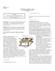
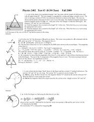
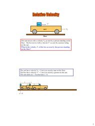
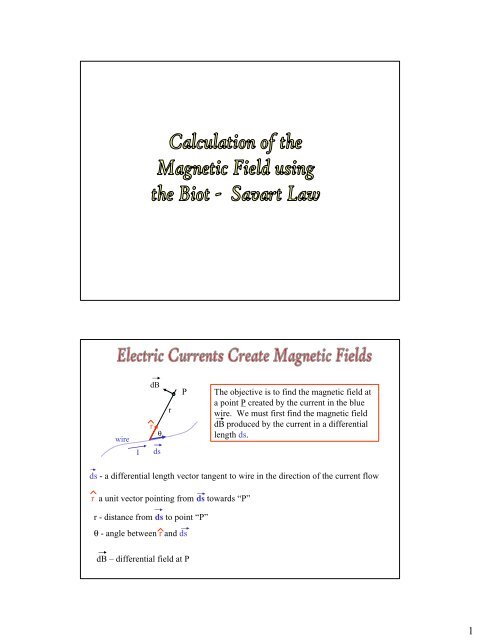
<strong>The</strong> objective is to find the magnetic field at<br />
a point P created by the current in the blue<br />
wire. We must first find the magnetic field<br />
dB produced by the current in a differential<br />
length ds.<br />
ds - a differential length vector tangent to wire in the direction of the current flow<br />
r a unit vector pointing from ds towards “P”<br />
r - distance from ds to point “P”<br />
θ - angle between r and ds<br />
dB – differential field at P<br />
1
wire<br />
I<br />
dB<br />
r<br />
r<br />
θ<br />
ds<br />
P<br />
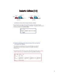
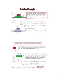
<strong>The</strong> differential field and its magnitude are:<br />
r<br />
d B =<br />
r<br />
µ<br />
4π<br />
r<br />
0 Id s × rˆ<br />
2<br />
µ 0 I sin θ ds<br />
dB =<br />
4π<br />
2<br />
r<br />
dB is perpendicular to both r and ds<br />
<strong>The</strong> field created by the complete wire would be obtained by<br />
integration of dB over the whole wire.<br />
µ 0 = 4π x 10 -7 T.m A<br />
Y<br />
wire<br />
ds<br />
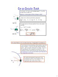
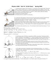
Step 1: Field dB due to current in ds:<br />
r<br />
r<br />
µ 0 Id s × rˆ<br />
d B =<br />
4π<br />
2<br />
r<br />
dθ<br />
θ<br />
r<br />
r<br />
I<br />
X<br />
<strong>The</strong> magnitude of ds is rdθ. <strong>The</strong> direction of<br />
the vector cross product is found from the<br />
RHR.<br />
dB<br />
^<br />
<strong>The</strong> direction is out of page in the +k direction:<br />
)<br />
ds<br />
× rˆ = krdθ ˆ<br />
r Id<br />
d B kˆ µ 0 θ<br />
=<br />
4π<br />
r<br />
2
Y<br />
θ = π/2<br />
ds<br />
Step 2: Integrate to find the total field. <strong>The</strong><br />
integration limits are zero to π/2.<br />
dθ<br />
r<br />
r<br />
I<br />
θ<br />
X<br />
B θ = 0<br />
B is out of the page<br />
r<br />
B<br />
π<br />
r kˆ<br />
2<br />
µ I kˆ<br />
0 µ I<br />
π<br />
0 2<br />
= ∫ dB = dθ<br />
= [ θ ]<br />
0<br />
4πr<br />
∫<br />
4πr<br />
0<br />
I<br />
kˆ<br />
µ 0<br />
=<br />
8r<br />
constants<br />
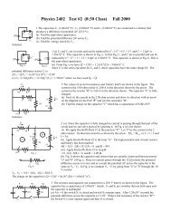
P<br />
wire<br />
r^<br />
ds<br />
I<br />
<strong>The</strong> field at P created by the current in the small length ds of<br />
the current carrying wire is zero since:<br />
ds<br />
r × rˆ = dssin 180 =<br />
( ) 0<br />
<strong>The</strong> total field created by the complete straight line segment is zero.<br />
3
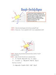
Field of a Straight Wire at an Off-Axis Point<br />
P<br />
Y<br />
a<br />
wire<br />
L 1<br />
I L 2<br />
X<br />
We want to find the magnetic field at the location P (0,a)<br />
created by the current in a straight wire located along the X<br />
axis from L 1 to L 2 .<br />
P<br />
a<br />
Y<br />
r = (x 2 + a 2 ) 1/2<br />
r^<br />
180-θ θ ds X<br />
L<br />
x<br />
1<br />
L 2<br />
Step 1: We find the field caused by the<br />
current in ds. Using the RHR:<br />
r<br />
d s × rˆ<br />
= kˆ<br />
( dssinθ<br />
)<br />
We replace ds by dx and sinθ by:<br />
sin<br />
( θ ) = sin( 180−θ)<br />
=<br />
a<br />
r<br />
r<br />
dB =<br />
µ 0<br />
4π<br />
v<br />
Ids × rˆ<br />
r<br />
2<br />
ˆ µ 0Idx<br />
⎛ a<br />
= k<br />
2<br />
⎜<br />
4πr<br />
⎝ r<br />
⎞<br />
⎟<br />
⎠<br />
ˆ µ 0Iadx<br />
= k<br />
3<br />
4πr<br />
= kˆ<br />
4π<br />
µ<br />
Iadx<br />
0<br />
3<br />
2 2<br />
( x + a )2<br />
4
B<br />
We integrate dB over the limits x = L 1 to x = L 2 :<br />
L<br />
r<br />
2<br />
ˆ µ 0Ia<br />
= ∫ dB = k<br />
4π<br />
∫<br />
L<br />
r ⎡<br />
= ˆ µ 0I<br />
B k ⎢<br />
4πa<br />
⎢<br />
⎣<br />
1<br />
dx<br />
ˆ µ 0Ia<br />
⎡<br />
= k ⎢<br />
( ) 3 4π<br />
2 2<br />
⎢ 2 2 2<br />
x + a 2 ⎣a<br />
( x + a )<br />
L<br />
−<br />
2<br />
( + ) 1<br />
( + ) 1<br />
⎥⎥ 2 2 2 2<br />
L a L1<br />
a ⎦<br />
2<br />
2<br />
2<br />
Usually it is more convenient to obtain the magnitude of this field from the<br />
following equation and obtain the correct direction from a new right hand rule<br />
shown on the next slide.<br />
L<br />
1<br />
⎤<br />
x<br />
1<br />
2<br />
⎤<br />
⎥<br />
⎥<br />
⎦<br />
L<br />
L<br />
2<br />
1<br />
µ 0I<br />
B =<br />
4 π a<br />
L<br />
1<br />
2<br />
( ) 1<br />
2 2 2<br />
L + a ( L + a ) 2<br />
2<br />
2<br />
2<br />
−<br />
1<br />
L<br />
1<br />
B<br />
B<br />
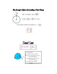
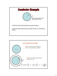
<strong>The</strong>se diagrams shown end views of two straight wires.<br />
<strong>The</strong> top wire has a current directed out of the page while the<br />
bottom wire has a current into the page. <strong>The</strong> magnetic field<br />
is circular about each wire. <strong>The</strong> direction is easily obtained<br />
from a new RHR of convenience.<br />
X<br />
Imagine grasping the wire <strong>with</strong> your right hand<br />
<strong>with</strong> your thumb extended in the current direction.<br />
Your fingers will wrap around the wire in the<br />
direction of the circular magnetic field.<br />
5
L 1<br />
= -L<br />
P<br />
a<br />
L>>a<br />
L 2<br />
= L<br />
µ 0 I<br />
B =<br />
4 π a<br />
1<br />
2 2<br />
( ) 1<br />
2 2 2<br />
L + a ( L + a ) 2<br />
2<br />
L<br />
2<br />
−<br />
1<br />
L<br />
1<br />
µ<br />
0I<br />
B =<br />
4πa<br />
L<br />
−<br />
− L<br />
µ<br />
≈<br />
L<br />
L<br />
− L<br />
−<br />
2 2<br />
( L + a ) 1<br />
2 2 2<br />
( L + a ) 1<br />
2<br />
4πa<br />
L<br />
0<br />
I<br />
µ 0I<br />
B =<br />
2πa<br />
As long as we are not too close to either end.<br />
6