Friction Laws and Work-Energy with Non Conservative Forces

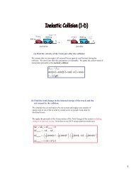
D. ShawVillanova UniversityMay 8, 2008Frictional Forces and Work – EnergyFor a Non Conservative ForceFall 2008ReminderYou must have your own notebook with your ownindividual conclusions. You must also submit your ownindividual formal reports.f k= m g +( m m ) ...( 1)The normal force exerted on the block by the horizontalsurface is:F N= m 2g1−1 2a...( 2)Introduction: The laws of static, kinetic and rolling frictionare investigated. A second very important objective is tostudy the Work – Energy Method when non conservativeresistive forces act.Equipment: Pasco dual range motion sensor, Pasco pulley,Pasco force sensor, Pasco cart, block with rubber surface,wooden plank, small spirit level, mass hanger with mass setand a few scales.Part A: Indirect Measurement of the Kinetic FrictionForceTheory: The hanging mass “m 1 ” in Fig.1 provides the force required toaccelerate the block along the table’ssurface. Our model includes a kineticfrictional force acting on the slidingblock. This frictional force is assumedto be independent of the speed of theblock. In the figure "m b " is the mass ofthe wood block and "m a " is the massincluded on top of the block. The totalmass of the block and included mass ism 2 = m b + m a . The block is connected bya cord passing over the Pasco pulley to amass hanger. The pulley is considered to be ideal with nokinetic energy or frictional force in the axle. The mass of thehanger and any additional mass supported by the hanger is m 1 .If the mass m 1 is sufficiently large it will be observed to movedownwards when released. By applying Newton's Second Lawto the motion of each object and letting “T” be the cordtension, “a” be the acceleration of both objects and “f k ” be thekinetic frictional force we have:m1g −T= m1aT − f = m ak 2By eliminating the tension we have:motionsensoradded masses (m a )m 2 = m b + m ablock (m b )plankdsIndirect MethodFig. 1Experiment and Analysis:• Record the mass of the wooden block “m b ” in kg.• Connect the wires from the motion sensor to the digitalchannels 1 and 2. The wire with the yellow tape (or with theyellow plug) goes to channel 1. Set the switch on the motionsensor to the wide angle position.• Click on the digital input 1 icon. A window showing theavailable sensors will open. Select the motion sensor in thislist. Select both the position and velocity to record andchoose a sample rate of 50 (Hz). You may have to reduce thisdata rate if you have difficulty obtaining good data. Use theSampling Options button to set a data collection time of 2.0seconds. Reminder: The motion sensor does NOT have to becalibrated under normal conditions. Inpulleym 1setting up the software DO NOT click onthe calibrate tab.• Drag and drop the velocity data icon fromthe Data Column on the Plot Icon in theDisplays Column. Also drag the distancedata icon from the Data Column and droponto the graph you just opened.•Place the block m b with the wood sidedown on the horizontal wooden board withno added mass on top of the block(m a = 0). Adjust the height of the pulley sothat the string between the pulley and theblock is as level as possible.• The string must be long enough so that when the block isabout .15 m from the pulley the hanging mass is just touchingthe floor. When the block is moved as far away from thepulley as possible (without the mass hanger touching thepulley) the distance from the block to the motion sensorshould be about 0.15m.• Select a hanging mass m 1 . This mass should be large enoughso that the system will move by itself when released from rest.Move the block as far from the pulley as possible without themass hanger touching the pulley. Click on the Start button andthen release the block when you here clicks from the motionsensor. You should try and move your hand very rapidly fromthe motion sensor's field of view to avoid false reflectionsfrom your hand and catch the block before it strikes the pulley.

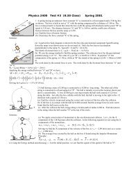
The acceleration of the system should be reasonably large tominimize errors caused by neglecting the inertial and frictionaleffects of the pulley wheel. Ignoring the data obtained beforethe block was released and after it was stopped, obtain the bestlinear fit to the velocity time graph. Record the accelerationwhich is the slope of this graph. The acceleration should be atleast 0.75 m/s 2 . If your acceleration is too small increase thehanging mass m 1 and try again. Record the values of m b andm 1 .• Do five more runs using different masses on top of the cart.Use the following values of m a : .150,.200, .300, .400 and .500 (kg). Ineach case use a value for m 1 that willgive an acceleration of at least 0.75m/s 2 . Be sure to record the values forthe acceleration and the masses m b , m aand m 1 in kilograms.• For many materials, under certainrestrictions, the kinetic frictional force,the normal force and the coefficient ofkinetic friction, μ k , are related by theempirical equation:fk= μ FkN...()3motionsensor• Open an Excel worksheet. Enter your measured values of“m 1 ”, “m a ” and “a” in successive columns. In the next columncalculate “m 2 ” which is m a + m b . In the next column computethe kinetic frictional force “f k ” using Eq. (1). Calculate thenormal force from Eq. (2) in the next column. Finallycompute, in the last column, the coefficient of kinetic friction“μ k ” from Equations (2) and (3).• Determine both the average value and standard deviation foryour measured values of the coefficient of kinetic friction. Theaverage of a range of cells from G2 to G7 is:AVERAGE(G2:G7)and the standard deviation is:STDEV(G2:G7).• Plot f k (Y axis) versus F N (X axis). Does your data appear toconfirm Eq. (3)? Select the Excel fitting option Y= mX (notY=mX+b). Graphically determine the coefficient of kineticfriction. Compare the graphical value with the mean valueobtained directly from Eq. (3) and compute the percentdifference. If you use the option Y=mX+b the slope and meanvalues may be different by an amount larger than you mighthave expected. Why?• After you finish the calculations for parts (i) and (ii), print acopy of your Excel work sheet along with the plot.Part B: Work – Energy Method with a Non ConservativeForceTheory: The sum of the kinetic and potential energies of asystem having only conservative forces doing work mustremain constant. Such a system was studied in the previousd idi m bim 1Work - EnergyFig. 2experiment. However, if a non conservative force such askinetic friction acts on the system, the sum of the kinetic andpotential energies does change. If we let “E” be the sum ofthe kinetic and potential energies, the Work – EnergyPrinciple with non conservative forces states that:ΔK + ΔU= W ⇒ ΔE=fW f...( 4)The data to test the Work – Energy Principle is obtained withthe method used in Part A. The only change is in the way weanalyze the data.Experiment and Analysis:Use the wood block by itself with noadded masses on top. For the hangingmass, try a total mass of .150 (kg).• Fig.2 shows the initial positions ofthe wood block and hanging massbefore they were released. Thedistance “d” is the distance to the blockrecorded by the motion sensor. Sincethe potential energy of the block doesnot change we only need to considerthe potential energy of the hangingmass. We can choose the zero reference position (where Uand y are both zero) for the gravitational potential of thehanging mass to be anywhere. We choose the referenceposition to be a distance “d i ” above the initial position of thehanging mass. Since the positive direction for the “Y” axis is“up”, the position of the hanging mass relative to ourreference position is “-d”. When the block of wood hasmoved a distance "d" from the motion sensor we assume thatits speed is "v". The hanging mass at this instant is a distance"d" below its reference position and from Fig.2 we see that:y = −d...( 5)At the instant the block of wood has moved a distance "d"from the motion sensor and both masses are moving with thespeed "v", the kinetic and potential energies are:1 2= ( ) ...( 6)2m m v 1= m gy = −m...( 7)K b +Uy = 0y = -d1 1gdThe kinetic energy of the system will increase as the hangingmass descends while the potential energy of the hanging masswill decrease. If the resistive forces did negligible work, thetotal energy would remain constant.• Use the same settings for Data Studio that you used in PartA but in addition drag the position data icon and drop it on topof your velocity graph. Check to see that the data collectionrate has not been inadvertently reset to 10 (hz).• Place the block of wood in position so the mass hanger isjust below the pulley and the block is about 0.20 (m) from themotion sensor. Click on Start and after you hear clicks from

the motion sensor release the block and move your hand out ofthe way as fast as possible. Be sure to catch the block before itcollides with the pulley. If the block seems to be moving tooslowly or too quickly you should change the hanging mass.•Examine the velocity versus time graph very carefully. Thevelocity should start at zero and then at some later time beginto increase in a uniform linear fashion (from zero) with time.However, it is possible that the velocity curve may suddenlyjump from zero to some other value before it increaseslinearly. This often happens when you do not move your handrapidly away from the block after the Start button is clicked.Also the data should be as smooth as possible (which mightrequire changing the hanging mass, reducing the datacollection rate, improving the alignment of the motion sensoror changing the wide and narrow angle motion sensor modes.)Since you only need one data set to analyze for this part of theexperiment it is important to have the best possible data set.Check with your instructor if you are not sure your data issatisfactory.• You may find that the velocities measured just after theblock began to move are not very smooth. If this is the case,make a note of the time at which the data begins to increaseuniformly so that earlier data can be removed in Excel.• Construct a data table for the distance by dragging yourdistance data and dropping it on the table icon. In the sameway construct a second table for the velocity measurements.Go to your distance data table and highlight all of the time anddistance values by moving the cursor to the top of the datatable where it should turn into a down arrow. Click and all ofyour distance and time data will be highlighted. Copy this datato the clipboard and transfer it to columns A and B of an Excelworksheet by pasting. Return to Data Studio and using thesame method copy and transfer the velocity and time data tothe same Excel worksheet in columns C and D.• Delete all of your data in columns A , B,C and D that wererecorded for times before the velocity data began to increaselinearly and smoothly. Similarly delete all data that occurredafter you stopped the block. You will notice that the times forthe distances and velocities are not the same since the velocityis computed from the distance measurements and therefore isobtained at a time halfway between two successive distancemeasurements. By cutting and pasting align the velocity andcorresponding time columns as closely as possible with thedistance and its corresponding time columns.• Use columns E, F and G for the calculation of K, U and Erespectively. Compute the kinetic and potential energies usingequations 6 and 7. Examine the energies in your worksheetcarefully. The kinetic energy should increase with time, whilethe potential energy decreases. The total energy will decreasesince the kinetic friction force does significant work. If yourdata is inconsistent with these general observations you needto check your measurements or calculations.• The forces acting on the block and hanging mass areassumed to be constant. The work done by these forces isdetermined by the product of the force, the distance movedand the cosine of the angle between the force and thedisplacement. Therefore the work done depends linearly onthe distance. Since the work done determines the change inthe kinetic energy of the system, the kinetic energy mustdepend linearly on the distance. The potential energy of thehanging mass is “-mgd” and also depends linearly on thedistance. Since the kinetic and potential energies are expectedto be linear with distance, plot on a single graph the kinetic,potential and total energy as functions of the distance, not thetime. Be sure to use the scatter plot option not the line option.To place multiple plots on the same graph use the add optionbelow the series box. Check your X axis scale carefully.Your values should all be less than 1 meter. If your axishas values greater than one meter you have made an error.(Most likely you have used the line option rather than thescatter option.)• Examine the plots carefully. Do your measurements confirmin a qualitative fashion the Work – Energy Method when anon conservative force does work? Explain. Do a linear fit ofthe total energy versus distance plot. The slope should benegative indicating that the kinetic frictional force has causeda decrease in the total mechanical energy “E”. If the force ofkinetic friction f k acts on the block over a distance “ds”, thenthe work done by this force is:dW = f cosθds= − fkdsThe work done by this force causes a change in the totalenergy of the block:dW = dECombining these equations we obtain:f ds = −dEkPrint only your Excel Plots, NOT your data tables.⇒fkk= −dEdsAccording to this result, the negative slope of the total energyversus distance curve at any position must be the force ofkinetic friction. If the plot of total energy versus the distanceis linear then the slope of the tangent at any location isconstant and is the same as the slope of a linear fit which is theconstant kinetic friction force. From the slope of your linearfit, find the kinetic friction force acting on the block.• Using this frictional force and the known normal force onthe block, calculate the coefficient of kinetic friction betweenthe block and the plank. Find the percent difference betweenthis value and the mean value found in Part A.

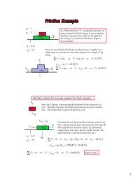
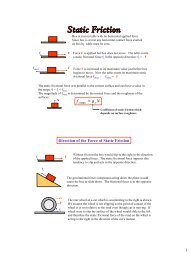
Part C: Direct Measurement of the Kinetic and StaticFrictional ForcesThe kinetic and static frictional forces can be measureddirectly using the force sensor as shown in Fig. 2. Forces to bemeasured are applied to the hook located at one end of theforce sensor. Connect the force sensor to channel A. Click onthe icon for Analog Channel A and select the force sensor (notthe student force sensor) from the list of available analogsensors and set the sample rate to 1000 (hz).• Calibration of the Force Sensor: The force sensor works bymeasuring the bending of a metal strip by the force applied toit. In order to measure forces accurately the sensor must firstbe calibrated.• Click the calibrate sensors tab and select the two pointcalibration. In the Calibration Point 1 area enter the value ofzero in the Standard Value Box. In the Calibration Point 2area enter the value of 10.29 in the Standard Value Box.• In the following steps you must hold the force sensor atrest in a vertical position. With nothing connected to theforce sensor press the TARE button on the sensor and thenclick on the Read from Sensor Button in the CalibrationPoint 1 area.• Press the TARE button againwith nothing connected to theforce sensor. Add an additionalmass of 1.00 (kg) to the masshanger for a total mass of 1.05kg (corresponding to a totalgravitational force of 10.29 N).Holding the force sensorvertically, connect the masshanger to the force sensor’shook and then click on the Readfrom Sensor Button in theForcestaticf s(max)kineticDirect MethodFig. 4timeCalibration Point 2 area. Finally click OK to exit thecalibration procedure.• Click on the Sampling Option tab and select a data collectiontime of 10 seconds and open a plot window to display theforce.• It is important to verify that the force sensor is workingcorrectly. Holding the force sensor vertically with nothingconnected to it, press the TARE button and collect data for afew seconds and then connect the hanger with the 1.00 (kg)added mass to the force sensor. The graph should indicate anet force of zero while nothing was connected and 10.3 (N)with the hanger and added 1.00 kg mass connected. If you donot obtain these values you need to repeat the calibrationprocess. Include a copy of the calibration plot with yourreport.• Attach a short string between the hook on the force sensorand the block which should be placed on the plank with thewood side down. Place masses on top of the block so that thetotal mass of the block plus added masses is about 1.5kilogram.• Press the TARE button on the force sensor with no forceapplied and then pull horizontally on the force sensor to applya force to the block. Begin with a very small force and veryslowly increase it until the block begins to move. Continue topull with the reduced force required to keep the block movingmore or less uniformly without accelerating. The graph of theapplied force versus time may be similar to Fig. 3.• The maximum force applied just before the block moved isthe maximum force of static friction f s(max) while the meanvalue of the force as the block moves with a constant speed isthe force of kinetic friction. Using the Smart Tool find f s(max)and f k . Determine the coefficients of static and kinetic frictionusing Eq. 2 to compute the normal force and Eq. 3 to obtainthe coefficients of friction.• Do a few more trials and obtain mean values and standarddeviations for the coefficients of static and kinetic friction.• Comment on the relative values of μ s and μ k .• Compare your values of μ k obtained using the two differentmethods of Part A and Part C. Assume the error in eachmethod is twice the standard deviation. Taking these errorsinto account are methods "A" and "C" consistent? However,the standard deviation is only a measure of random errors anddoes not include any systematic errors in the experiment.Part D: The Force of Rolling FrictionIntroduction: When the wheel of a car moves along a flatroad it will experience a kinetic frictional force if the wheel isslipping. If the car is speeding up or slowing down withoutslipping (or even moving with a constant velocity against anair resistive force) astatic frictional force actson the wheel. In additionto these frictional forcesthere is a third type offrictional force known asrolling friction. Rollingfriction between asurface and a wheel isθdue to deformation of the surface and the wheel itself andadhesion (stickiness) of the surfaces. As deformation of theflat surface and the wheel occur, a resistive force developssince the wheel has to “plow its way” through the surface.The resistive rolling frictional force follows an empirical lawthat is the same as for kinetic friction:froll= μ FrN...( 8)where μ r is the coefficient of rolling friction. The coefficientof rolling friction is usually much smaller than the coefficientof kinetic friction. For example, the coefficients of kinetic androlling friction for a steel railway car wheel on a steel rail areapproximately 0.2 and .001 respectively.Experimental: In this part of the experiment the coefficientof rolling coefficient of friction is measured for a cart. Thevalue obtained includes the rolling friction at each wheel asf rollF NmgmgcosθRolling FrictionFig. 5mgsinθ

well as any kinetic friction in the wheel bearings. Since therolling frictional force is very small, we should minimize thecontribution of other forces, such as gravity, that would tendto obscure the rolling frictional force. Ideally the plank shouldbe level to eliminate the gravitational force component.However, if the plank is not perfectly level, a smallgravitational force component will act on the cart in adirection parallel to the plank. We remove the possibleinfluence of gravity by measuring the acceleration of the cartfor motion in both directions. The cart is placed on the plankalong with the motion sensor and given a gentle push. Theacceleration is measured a few times. Then the cart is pushedin the opposite direction and its acceleration measured. Fromthese values we can obtain the coefficient of rolling frictionfor the cart.The cart is shown in Fig. 4. We have assumed that the tabletop may be tilted by a very small angle θ from the horizontal.When the cart is given a gentle push to the right we let itsacceleration be “a r ” and we choose the positive direction to betowards the right. The gravitational force component“mgsinθ” is smaller than the frictional force and the cart slowsdown even though it may be going down a slight hill. Weapply Newton’s II Law to the free body diagram shown:() 9FN= mg cosθ...mg sinθ− f = marollr...( 10)When the cart is pushed to the left we take the positivedirection to the left and both the frictional and gravitationalforces slow the cart down:− mg sinθ− f roll= mal...( 11)We solve equations (10) and (11) for the force of rollingfriction:froll− m ar=2( + a )l...( 12)• Place the motion sensor to the left of the cart and give thecart a gentle push to the right. Use the motion sensor to recordits velocity for three seconds. Do a linear fit to find theacceleration of the cart. Obtain at least three measurements ofthe acceleration “a r ” and find the average value. Note that thisvalue should be negative.• Place the motion sensor to the right of the cart and push thecart gently to the left and obtain at least three values of theacceleration “a l ”. Find the average which should also benegative.• Compute the coefficient of rolling friction of the cart usingEq. 13.How does the coefficient of rolling friction of the cartcompare with the coefficient of kinetic friction of the slidingblock?Check List: Minimal Requirements for Lab Notebook ReportThe significance of each graph must be discussed and the fitted values(such as the intercept and slope) must be compared with model valueswhen possible.Part A: Excel Data Table with masses used, calculated normal force,calculated frictional force and the coefficient of kinetic friction. Plot of kinetic frictional force versus the normal force with a linearfit through the origin. The % difference between the coefficient ofkinetic friction from the graph and the mean table value. Copy of one Data Studio plot of speed versus time.Part B: A copy of a few rows of your excel sheet displaying the distance,speed and energies. Plot of the kinetic, potential and total energy versus distance with alinear fit of the total energy curve. The value of the coefficient of kinetic friction obtained from the fit.Part C: Data Studio plot of the force applied by the force sensor versus time. The maximum force of static friction and the mean force of kineticfriction obtained from this plot. The coefficients of static and kinetic friction found from the abovefrictional forces. Compare the mean frictional force found in C with mean value foundin A and the value obtained in B. Discussion of these results.The coefficient of rolling friction is:μrollf=FrollN( a + a ) − ( a + a )−r lr= ≈2gcosθ2gl...( 13)Part D: Excel data table for measured accelerations and the computed valuefor the coefficient of rolling friction. Discussion.ConclusionsSince θ is a very small angle its cosine is very close to one.