Friction Laws and Work-Energy with Non Conservative Forces

More documents

Recommendations

Info

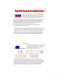
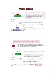
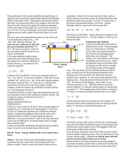
The acceleration of the system should be reasonably large tominimize errors caused by neglecting the inertial and frictionaleffects of the pulley wheel. Ignoring the data obtained beforethe block was released and after it was stopped, obtain the bestlinear fit to the velocity time graph. Record the accelerationwhich is the slope of this graph. The acceleration should be atleast 0.75 m/s 2 . If your acceleration is too small increase thehanging mass m 1 and try again. Record the values of m b andm 1 .• Do five more runs using different masses on top of the cart.Use the following values of m a : .150,.200, .300, .400 and .500 (kg). Ineach case use a value for m 1 that willgive an acceleration of at least 0.75m/s 2 . Be sure to record the values forthe acceleration and the masses m b , m aand m 1 in kilograms.• For many materials, under certainrestrictions, the kinetic frictional force,the normal force and the coefficient ofkinetic friction, μ k , are related by theempirical equation:fk= μ FkN...()3motionsensor• Open an Excel worksheet. Enter your measured values of“m 1 ”, “m a ” and “a” in successive columns. In the next columncalculate “m 2 ” which is m a + m b . In the next column computethe kinetic frictional force “f k ” using Eq. (1). Calculate thenormal force from Eq. (2) in the next column. Finallycompute, in the last column, the coefficient of kinetic friction“μ k ” from Equations (2) and (3).• Determine both the average value and standard deviation foryour measured values of the coefficient of kinetic friction. Theaverage of a range of cells from G2 to G7 is:AVERAGE(G2:G7)and the standard deviation is:STDEV(G2:G7).• Plot f k (Y axis) versus F N (X axis). Does your data appear toconfirm Eq. (3)? Select the Excel fitting option Y= mX (notY=mX+b). Graphically determine the coefficient of kineticfriction. Compare the graphical value with the mean valueobtained directly from Eq. (3) and compute the percentdifference. If you use the option Y=mX+b the slope and meanvalues may be different by an amount larger than you mighthave expected. Why?• After you finish the calculations for parts (i) and (ii), print acopy of your Excel work sheet along with the plot.Part B: Work – Energy Method with a Non ConservativeForceTheory: The sum of the kinetic and potential energies of asystem having only conservative forces doing work mustremain constant. Such a system was studied in the previousd idi m bim 1Work - EnergyFig. 2experiment. However, if a non conservative force such askinetic friction acts on the system, the sum of the kinetic andpotential energies does change. If we let “E” be the sum ofthe kinetic and potential energies, the Work – EnergyPrinciple with non conservative forces states that:ΔK + ΔU= W ⇒ ΔE=fW f...( 4)The data to test the Work – Energy Principle is obtained withthe method used in Part A. The only change is in the way weanalyze the data.Experiment and Analysis:Use the wood block by itself with noadded masses on top. For the hangingmass, try a total mass of .150 (kg).• Fig.2 shows the initial positions ofthe wood block and hanging massbefore they were released. Thedistance “d” is the distance to the blockrecorded by the motion sensor. Sincethe potential energy of the block doesnot change we only need to considerthe potential energy of the hangingmass. We can choose the zero reference position (where Uand y are both zero) for the gravitational potential of thehanging mass to be anywhere. We choose the referenceposition to be a distance “d i ” above the initial position of thehanging mass. Since the positive direction for the “Y” axis is“up”, the position of the hanging mass relative to ourreference position is “-d”. When the block of wood hasmoved a distance "d" from the motion sensor we assume thatits speed is "v". The hanging mass at this instant is a distance"d" below its reference position and from Fig.2 we see that:y = −d...( 5)At the instant the block of wood has moved a distance "d"from the motion sensor and both masses are moving with thespeed "v", the kinetic and potential energies are:1 2= ( ) ...( 6)2m m v 1= m gy = −m...( 7)K b +Uy = 0y = -d1 1gdThe kinetic energy of the system will increase as the hangingmass descends while the potential energy of the hanging masswill decrease. If the resistive forces did negligible work, thetotal energy would remain constant.• Use the same settings for Data Studio that you used in PartA but in addition drag the position data icon and drop it on topof your velocity graph. Check to see that the data collectionrate has not been inadvertently reset to 10 (hz).• Place the block of wood in position so the mass hanger isjust below the pulley and the block is about 0.20 (m) from themotion sensor. Click on Start and after you hear clicks from
the motion sensor release the block and move your hand out ofthe way as fast as possible. Be sure to catch the block before itcollides with the pulley. If the block seems to be moving tooslowly or too quickly you should change the hanging mass.•Examine the velocity versus time graph very carefully. Thevelocity should start at zero and then at some later time beginto increase in a uniform linear fashion (from zero) with time.However, it is possible that the velocity curve may suddenlyjump from zero to some other value before it increaseslinearly. This often happens when you do not move your handrapidly away from the block after the Start button is clicked.Also the data should be as smooth as possible (which mightrequire changing the hanging mass, reducing the datacollection rate, improving the alignment of the motion sensoror changing the wide and narrow angle motion sensor modes.)Since you only need one data set to analyze for this part of theexperiment it is important to have the best possible data set.Check with your instructor if you are not sure your data issatisfactory.• You may find that the velocities measured just after theblock began to move are not very smooth. If this is the case,make a note of the time at which the data begins to increaseuniformly so that earlier data can be removed in Excel.• Construct a data table for the distance by dragging yourdistance data and dropping it on the table icon. In the sameway construct a second table for the velocity measurements.Go to your distance data table and highlight all of the time anddistance values by moving the cursor to the top of the datatable where it should turn into a down arrow. Click and all ofyour distance and time data will be highlighted. Copy this datato the clipboard and transfer it to columns A and B of an Excelworksheet by pasting. Return to Data Studio and using thesame method copy and transfer the velocity and time data tothe same Excel worksheet in columns C and D.• Delete all of your data in columns A , B,C and D that wererecorded for times before the velocity data began to increaselinearly and smoothly. Similarly delete all data that occurredafter you stopped the block. You will notice that the times forthe distances and velocities are not the same since the velocityis computed from the distance measurements and therefore isobtained at a time halfway between two successive distancemeasurements. By cutting and pasting align the velocity andcorresponding time columns as closely as possible with thedistance and its corresponding time columns.• Use columns E, F and G for the calculation of K, U and Erespectively. Compute the kinetic and potential energies usingequations 6 and 7. Examine the energies in your worksheetcarefully. The kinetic energy should increase with time, whilethe potential energy decreases. The total energy will decreasesince the kinetic friction force does significant work. If yourdata is inconsistent with these general observations you needto check your measurements or calculations.• The forces acting on the block and hanging mass areassumed to be constant. The work done by these forces isdetermined by the product of the force, the distance movedand the cosine of the angle between the force and thedisplacement. Therefore the work done depends linearly onthe distance. Since the work done determines the change inthe kinetic energy of the system, the kinetic energy mustdepend linearly on the distance. The potential energy of thehanging mass is “-mgd” and also depends linearly on thedistance. Since the kinetic and potential energies are expectedto be linear with distance, plot on a single graph the kinetic,potential and total energy as functions of the distance, not thetime. Be sure to use the scatter plot option not the line option.To place multiple plots on the same graph use the add optionbelow the series box. Check your X axis scale carefully.Your values should all be less than 1 meter. If your axishas values greater than one meter you have made an error.(Most likely you have used the line option rather than thescatter option.)• Examine the plots carefully. Do your measurements confirmin a qualitative fashion the Work – Energy Method when anon conservative force does work? Explain. Do a linear fit ofthe total energy versus distance plot. The slope should benegative indicating that the kinetic frictional force has causeda decrease in the total mechanical energy “E”. If the force ofkinetic friction f k acts on the block over a distance “ds”, thenthe work done by this force is:dW = f cosθds= − fkdsThe work done by this force causes a change in the totalenergy of the block:dW = dECombining these equations we obtain:f ds = −dEkPrint only your Excel Plots, NOT your data tables.⇒fkk= −dEdsAccording to this result, the negative slope of the total energyversus distance curve at any position must be the force ofkinetic friction. If the plot of total energy versus the distanceis linear then the slope of the tangent at any location isconstant and is the same as the slope of a linear fit which is theconstant kinetic friction force. From the slope of your linearfit, find the kinetic friction force acting on the block.• Using this frictional force and the known normal force onthe block, calculate the coefficient of kinetic friction betweenthe block and the plank. Find the percent difference betweenthis value and the mean value found in Part A.
Page 1: D. ShawVillanova UniversityMay 8, 2
Page 5: well as any kinetic friction in the

Friction Laws and Work-Energy with Non Conservative Forces

You also want an ePaper? Increase the reach of your titles

Delete template?

Save as template?