Modeling and control of a 4-wheel skid-steering ... - University of Haifa

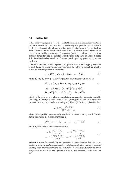
3.4 Control law
In this paper we propose to resolve control at kinematic level using algorithm based
on Dixon’s research. The more details concerning this approach can be found in
[5, 4, 13]. This controller allows to obtain practical stabilization [7], i.e. tracking
error is bounded to the assumed non zero value. The actual desired tunnel of errors
is determined by function δ d (t) = α 0 exp(α 1 t) + ε 1 , where α 0 ,α 1 > 0 are
constant parameters and ε 1 denotes desired steady-state value of vector z norm.
This function describes envelope of an additional signal z d generated by tunable
oscillator.
In order to extend kinematic algorithm at dynamic level a backstepping technique
is used. Based on Lyapunov analysis we propose the following control law which is
robust on dynamic parameter uncertainty
τ ¯B−1 (wJz + ˜z + Y d ϑ 0 + τ a + k 3 ũ) , (30)
where Y d (u d , ˙u d , ˜q,θ,q r ) ∈ R 2×6 represents known regression matrix as
¯M ˙u d + ¯Cud + ¯R = Yd (u d , ˙u d , ˜q,θ,q r ) ϑ, (31)
( )
¯M = T T ¯MT, ¯C = T
T ¯CT + ¯M T˙
,
(
¯R = T T ¯CΠ + ¯M ˙Π + ¯R
)
(32)
, ¯B = T
T ¯B,
with k 3 > 0, while u d is a velocity control signal generated by kinematic controller
(see [13]), ϑ and ϑ 0 are actual and a constant, best-guess estimation of dynamical
parameter vector, respectively. According to [14] and [5] the term τ a is defined as
ρ 2 Yd T
τ a Y ũ
d
∥ Y
T
d ũ ∥ , (33)
ρ + ε2
where ε 2 is a positive constant scalar which can be made arbitrary small. The dynamic
parameters in (31) are determined as
ϑ [ m I µ L µ R µ F µ B
] T
∈ R
6
(34)
with weighted friction coefficients defined as
µ L bµ s1 + aµ s2
, µ R bµ s4 + aµ s3
a + b
a + b
µ F 2a(µ l2 + µ l3 )
, µ B 2b(µ l1 + µ l4 )
a + b
a + b
Remark 4 It can be proved [10] that proposed kinematic control law and its extension
at dynamic level ensures practical stabilization yielding ultimately bounded
tracking error under assumptions that constraint (4) is satisfied, parameters uncertainty
is limited and trajectory signals are bounded that has been pointed in section
3.2.
(35)