Modeling and control of a 4-wheel skid-steering ... - University of Haifa

Modeling and control of a 4-wheel skid-steering
mobile robot: From theory to practice ∗
K. Kozłowski 1 , D. Pazderski 2 I.Rudas 3 , J.Tar 4
Poznań University of Technology
Budapest Polytechnic
ul. Piotrowo 3a Népszínház utca 8.
60-395 Poznań, Poland H-1081 Budapest, Hungary
1 Krzysztof.Kozlowski@put.poznan.pl 3 rudas@bmf.hu
2 Dariusz.Pazderski@put.poznan.pl 4 tar.jozsef@nik.bmf.hu
Abstract:
In this paper problem of modeling and control of 4-wheel skid-steering mobile robot is presented.
To obtain practical stabilization for both admissible and non-admissible trajectories
[13, 7, 8], i.e. trajectories which do not satisfy nonholonomic constraint, control scheme
which is based on kinematic algorithm [4, 5] is proposed. Theoretical considerations are
verified by numerical simulation and experiments. In addition some details concerning implementation
of proposed algorithm is given.
1 Introduction
Skid-steering mobile robots (SSMRs)
are quite different from classical wheeled mobile
robots for which lack of slippage is usually
supposed – see for example [3]. In addition
interaction between ground and wheels
makes their mathematical model to be uncertain
and caused control problem to be difficult
as it generally demands quite detailed
consideration of dynamic properties.
In this paper we propose to use a continuous
and time-differentiable control law which is
based on kinematic oscillator [5] to resolve
both regulation and trajectory tracking problem.
Here we refer to work done by Caracci-
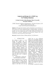
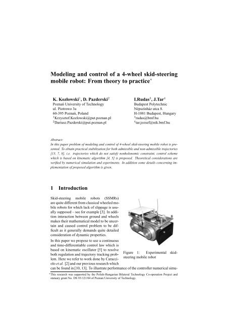
Figure 1: Experimental skidsteering
mobile robot
olo et al. [2] and our previous research which
can be found in [10, 13]. To illustrate performance of the controller numerical simu-
∗ This research was supported by the Polish-Hungarian Bilateral Technology Co-operation Project and
statuary grant No. DS 93/121/04 of Poznan University of Technology.

lations are presented. Next, experimental verification using small four-wheel SSMR
(see Fig. 1) is described and some results of experiments are given.
2 Model of the robot
2.1 Introduction
In this section kinematic and dynamic model of four-wheel skid-steering mobile
robot is presented. We refer to the real experimental construction consists of twowheel
differentially driven mobile robots namely MiniTracker 3 (see Fig.1) [9].
In order to simplify the mathematical model of SSMR we assume that [2]
• plane motion is considered only,
• achievable linear and angular velocities of the robot are relatively small,
• wheel contacts with surface at geometrical point (tire deformation is neglected),
• vertical forces acting on wheels are statically dependent on weight of the vehicle,
• viscous friction phenomenon is assumed to be negligible.
2.2 Kinematics
Firstly, consider a vehicle moving on two dimensional plane with inertial coordinate
frame (X g ,Y g ) as depicted in Fig. 1(a). To describe motion of the robot it is
convenient to define an local frame attached to it with origin in its center of mass
(COM). Assume that q [ X Y θ ] T
∈ R 3 denotes generalized coordinates,
where X, Y determine COM position and θ is an orientation the local frame with
respect to the inertial frame, respectively.
Let v [ ] T
v x v y ∈ R 2 be a velocity vector of COM expressed in the local
frame with v x and v y determining longitudinal and lateral velocity of the vehicle
[4].
From Fig. 1(a) it is easy to derive kinematic equation of motion using rotation matrix
as follows ⎡ ⎤ ⎡
⎤⎡
⎤
Ẋ cos θ −sin θ 0 v x
˙q = ⎣ Ẏ ⎦ = ⎣ sinθ cos θ 0 ⎦⎣
v y
⎦, (1)
˙θ 0 0 1 ω
where ˙q ∈ R 3 is the generalized velocity vector and ω denotes angular velocity of
the vehicle.

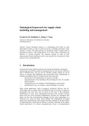
(a) Free-body kinematics
(b) Wheel velocities
relationships
Figure 2: Kinematics of SSMR
To complete kinematic model of SSMR additional velocity constraints should be
considered with respect to the inertial frame. According to geometrical situation
presented in Fig. 1(b) one can prove that coordinates of velocities of points P 1 ,
P 2 ,...,P 4 where the wheels of the robot touch the plane must satisfy [13, 12]
v L v 1x = v 2x , v R v 3x = v 4x ,
v F v 2y = v 3y , v B v 1y = v 4y ,
(2)
where v L , v R denote longitudinal coordinates of left and right wheel velocities, v F
and v B , are lateral coordinates of velocities of front and rear wheels, respectively.
Remark 1 From Fig. 1(b) it is clear [13, 12] that v iy is equal to zero for straight
motion only (i.e. if ω = 0), otherwise v iy ≠ 0 that implies lateral skid that is
necessary to change orientation of such vehicle.
Notice that ω L and ω R which denote angular velocities of left and right wheels,
respectively, can be regarded as control inputs at kinematic level and can be used to
control longitudinal and angular velocity according to the following relationships
v x = r ω L + ω R
2
, ω = r −ω L + ω R
, (3)
2c
while r is so called effective radius of wheels [11] and 2c is a spacing wheel track
depicted in Fig. 1(a).
Remark 2 It is very important to note that equations (3) are valid only if longitudinal
slip does not appear, otherwise they should be treated as just approximations
and to improve accuracy parameters c and r should be identified experimentally.
Next, lateral velocity v y which determines velocity of lateral slip of the vehicle can
be obtained as follows [13]
v y + x ICR ω = 0, (4)

where x ICR is a coordinate of instantaneous center of rotation (ICR) of the robot
expressed along x l axis. It can be proved that this equation in not integrable, hence
it describes nonholonomic constraint and can be written in Pfaffian form as
[
−sin θ cos θ xICR
] [
Ẋ Ẏ ˙θ
] T
= A(q) ˙q = 0, (5)
where equation (1) has been used. Since the generalized velocity ˙q is always in the
null space of A one can write that
˙q = S (q) η, (6)
where η ∈ R 2 is a control input at kinematic level defined as
η [ v x ω ] T
, (7)
S ∈ R 3×2 is the following matrix
⎡
S (q) = ⎣
cos θ x ICR sinθ
sin θ −x ICR cos θ
0 1
⎤
⎦ (8)
which satisfies
S T (q) A T (q) = 0. (9)
Remark 3 Equation (6) describes kinematics of SSMR which will be used to formulate
control law. Since dim(η) < dim(q) SSMR can be regarded as an underactuated
system. Furthermore, because of constraint (5) this system is nonholonomic.
2.3 Dynamics
Because of interaction between wheels and
ground dynamic properties of SSMR play a
very important role. It should be noted that
if the robot is changing its orientation reactive
friction forces are usually much higher
than forces resulting from inertia. As a consequence,
even for relatively low velocities,
dynamic properties of SSMR influence motion
much more than for other vehicles for
which non-slipping and pure rolling assumption
may be satisfied.
However in this section only simplified dynamics
of SSMR [2], which will be useful for
control purpose, are introduced. In order to
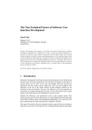
simplify this model we assume that the mass Figure 3: Forces and torques
distribution of the vehicle is almost homogeneous, kinetic energy of the wheels and

drives can be neglected and detailed description of tyre which can be found, for
example, in [11] are omitted.
A dynamic equation of SSMR can be obtained using Euler-Lagrange principle with
Lagrange multipliers to include nonholonomic constraint and it can be written as
M (q) ¨q + R ( ˙q) = B (q) τ + A T (q) λ, (10)
where M ∈ R 3×3 denotes the constant, diagonal, positive definite inertia matrix
⎡
m 0
⎤
0
M = ⎣ 0 m 0 ⎦ , (11)
0 0 I
m, I represent the mass and inertia, respectively, R ( ˙q) ∈ R 3 denotes vector of
resultant reactive forces F l , F s and torque M r
⎡
R ( ˙q) = ⎣ F ⎤
s ( ˙q) cos θ − F l ( ˙q) sinθ
F s ( ˙q) sin θ + F l ( ˙q) cos θ ⎦ , (12)
M r ( ˙q)
B ∈ R 3×2 denotes input matrix and is explicitly defined as follows
⎡ ⎤
B (q) = 1 cos θ cos θ
⎣ sin θ sin θ ⎦ . (13)
r
−c c
The term τ = [ ] T
τ L τ R ∈ R 2 which appears in (10) can be treated as a control
signal at dynamic level and represents torques generated by actuators on the left and
right side of the robot. Notice that these torques produce active forces F i (see Fig. 3)
that are theoretically independent on longitudinal slip.
The reactive forces and torque in (12) are calculated as
and
where
F s ( ˙q) =
4∑
F si ( ˙q) , F l ( ˙q) =
i=1
4∑
F li ( ˙q) (14)
i=1
M r ( ˙q) = b[F l2 ( ˙q) + F l3 ( ˙q)] − a[F l1 ( ˙q) + F l4 ( ˙q)]
+c[−F s1 ( ˙q) − F s2 ( ˙q) + F s3 ( ˙q) + F s4 ( ˙q)] (15)
F si ( ˙q) µ si N i sgn(v ix ) , F li ( ˙q) µ li N i sgn (v iy ) (16)
while µ si and µ li are dry friction coefficients for i th wheel in longitudinal and lateral
direction, respectively, N i is a reactive vertical force which acts on wheel and is
supposed to be statically dependent on weight of the vehicle (see [2]).

For control purpose it would be convenient to express dynamic equation in η and ˙η
terms. According to it one can obtain that
where relationships (6) and (9) have been used,
¯M ˙η + ¯Cη + ¯R = ¯Bτ, (17)
¯M = S T MS, ¯C = S T MṠ, ¯R = S T R, ¯B = S T B. (18)
3 Controller
3.1 Operational constraint
In previous section the constraint (4) was considered. However it is difficult to
measure or estimate x ICR value in practice. Therefore motivated by work done by
Caracciolo et al. [2] we put an artificial constraint based on (4) and assume that
x ICR = x 0 = const. It can be written as
v y + x 0 ω = 0, (19)
where x 0 ∈ (−a,b), while a and b are geometrical parameters depicted in Fig. 1(a).
This assumption is consequently used in control development and can be interpreted
as an outer-loop term in the controller which limits skid of the vehicle in lateral
direction [13].
3.2 Control objective
For control purposes the following tracking error is defined
˜q (t) [ ˜X (t) Ỹ (t) ˜θ (t)
] T
= q (t) − qr (t), (20)
where q r (t) = [ X r (t) Y r (t) θ r (t) ] T
denotes reference position and orientation.
We assume that for all times reference vector and its first and second time
derivative are bounded, i.e. q r (t), ˙q r (t), ¨q r (t) ∈ L ∞ . Here we do not imposed
any additional restriction on reference signal q r (regulation case can be considered,
too). Additionally, in opposite to the previous works [5, 4, 10, 13] we consider the
case for which q r is defined in a such way that velocities associated with it do not
satisfy nonholonomic constraints.
In order to facilitate subsequent control we determine kinematic error assuming that
the constraint (19) is satisfied. Next, taking the time derivative of equation (6) and
using relationship (9) one can conclude that
˙˜q (t) = S (q) η − ˙q r (t) . (21)

3.3 Position and velocity transformations
Kinematic controller based on Dixon’s scheme uses transformation which transforms
original system – in this case described by equation (21) – to an auxiliary
system (22) similar to nonholonomic Brockett’s integrator [1]
ẇ = u T J T z + f, ż = u, (22)
where variables w ∈ R 1 and z ∈ R 2 form three-dimensional state vector, u ∈ R 2 is
a new velocity control vector and f ∈ R 1 is a drift of the system, while J represents
a constant, skew symmetric matrix defined as
J =
[
0 −1
1 0
]
. (23)
It can be proved that following transformation defines global diffeomorphism with
respect to the origin
Z [ w z ] T T
= P
(θ, ˜θ
)
˜q, (24)
where
P
(
θ, ˜θ
)
=
⎡
⎣ −˜θ cos θ + 2sin θ p 12 = −˜θ sin θ − 2cos θ −2x 0
0 0 1
cos θ sin θ 0
⎤
⎦. (25)
Using this transformation and calculating auxiliary errors we can find velocity transformation
which relates velocity vector η with control signal u as follows
η = T (˜q,q) u + Π, (26)
where
T (˜q,q) =
[ L 1
1 0
]
(27)
is an invertible velocity transformation matrix, L = ˜X sinθ − Ỹ cos θ and
[ ]
ωr L +
Π(q,q r ,t) =
Ẋr cos θ + Ẏr sinθ
ω r
(28)
is a time-varying vector associated with reference trajectory. In the similar way we
can calculate drift term f as follows
(
)]
f = 2
[ω r x 0 + z 2 − Ẋr sinθ + Ẏr cos θ . (29)
Summarizing, the obtained velocity transformation allows to use kinematic controller
to resolve practical stabilization for admissible and non-admissible trajectories.

3.4 Control law
In this paper we propose to resolve control at kinematic level using algorithm based
on Dixon’s research. The more details concerning this approach can be found in
[5, 4, 13]. This controller allows to obtain practical stabilization [7], i.e. tracking
error is bounded to the assumed non zero value. The actual desired tunnel of errors
is determined by function δ d (t) = α 0 exp(α 1 t) + ε 1 , where α 0 ,α 1 > 0 are
constant parameters and ε 1 denotes desired steady-state value of vector z norm.
This function describes envelope of an additional signal z d generated by tunable
oscillator.
In order to extend kinematic algorithm at dynamic level a backstepping technique
is used. Based on Lyapunov analysis we propose the following control law which is
robust on dynamic parameter uncertainty
τ ¯B−1 (wJz + ˜z + Y d ϑ 0 + τ a + k 3 ũ) , (30)
where Y d (u d , ˙u d , ˜q,θ,q r ) ∈ R 2×6 represents known regression matrix as
¯M ˙u d + ¯Cud + ¯R = Yd (u d , ˙u d , ˜q,θ,q r ) ϑ, (31)
( )
¯M = T T ¯MT, ¯C = T
T ¯CT + ¯M T˙
,
(
¯R = T T ¯CΠ + ¯M ˙Π + ¯R
)
(32)
, ¯B = T
T ¯B,
with k 3 > 0, while u d is a velocity control signal generated by kinematic controller
(see [13]), ϑ and ϑ 0 are actual and a constant, best-guess estimation of dynamical
parameter vector, respectively. According to [14] and [5] the term τ a is defined as
ρ 2 Yd T
τ a Y ũ
d
∥ Y
T
d ũ ∥ , (33)
ρ + ε2
where ε 2 is a positive constant scalar which can be made arbitrary small. The dynamic
parameters in (31) are determined as
ϑ [ m I µ L µ R µ F µ B
] T
∈ R
6
(34)
with weighted friction coefficients defined as
µ L bµ s1 + aµ s2
, µ R bµ s4 + aµ s3
a + b
a + b
µ F 2a(µ l2 + µ l3 )
, µ B 2b(µ l1 + µ l4 )
a + b
a + b
Remark 4 It can be proved [10] that proposed kinematic control law and its extension
at dynamic level ensures practical stabilization yielding ultimately bounded
tracking error under assumptions that constraint (4) is satisfied, parameters uncertainty
is limited and trajectory signals are bounded that has been pointed in section
3.2.
(35)

4 Simulation results
In this section we present simulation results performed in Matlab/Simulink environment
to verify behavior of the controller. The parameters of the SSMR model
were chosen to correspond as closely as possible to the real experimental robot presented
in section 1 in the following manner: a = b = 0.039[m], c = 0.034[m],
r = 0.0265[m], m = 1[kg], I = 0.0036[kg · m 2 ].
Permissible torque signal and angular velocities of wheels were saturated as:
τ max = 0.25[Nm], ω max = 56[rad/s]. Friction parameters of the surface µ si
and µ li were modeled using scalar functions depending on actual position of center
of i th wheel expressed in the inertial frame and were supposed to be bounded as
follows: 0.02 ≤ µ si ≤ 0.18, 0.2 ≤ µ li ≤ 0.8.
Remark 5 For comparison purpose initial conditions and the parameters assumed
in simulations correspond to those used in experiments which are described in section
5.
Firstly, regulation problem is examined. The initial posture error was selected as
˜q (0) = [ 0 0.5 −π/4 ] T
. The control gains were given as k1 = 0.5, k 2 = 0.5,
k 3 = 10, while coefficients which determine accuracy in steady-state were ε 1 =
0.01 and ε 2 = 0.1. The oscillator signal was initialized as follows
z d (0) = 1.5 [ cos (−π/3)
sin(−π/3) ] T
and the coefficient which determines desired convergence of errors was selected as
α 1 = 0.4.
The best-guess estimates of mass and inertia were 20 and 50 percent higher, respectively,
than parameters assumed for the robot model. Next, estimates of friction
coefficients were selected as µ L0 = µ R0 = 0.1 and µ F0 = µ B0 = 0.5, while
bounding coefficient ρ = 1. Furthermore, the constant x 0 related to ICR position
was assumed to be equal to −0.02[m].
In Fig. 3(a) performed trajectory in Cartesian space is depicted and the position and
orientation is marked at every second of simulation. From Fig. 3(b) it is clear that
initial errors are significant reduced and in steady-state are bounded as follows
∣ ˜X
∣ < 5[mm],
∣
∣Ỹ
∣ < 5[mm],
∣
∣˜θ
∣ < 0.01[rad].
It is worth to note that convergence to the set of permissible errors is exponential.
In the next simulation trajectory tracking were examined. The sinusoidal admissible
reference trajectory were selected as
X r = 0.1t [m],
Y r = 0.3sin (0.6t) [m],
while θ r was numerically calculated to satisfy the constraint (19). The initial oscillator
signal was selected as
z d (0) = 0.4 [ cos (−π/2)
sin(−π/2) ] T

Y [m]
0.6
0.5
0.4
0.3
0.2
0.1
0
q(t)
q r
(t)
q(0)
q r
(0)
−0.1
−0.6 −0.4 −0.2 0 0.2 0.4
X [m]
(a) Performed trajectory
X−X r
[m], Y−Y r
[m], θ−θ r
[rad]
1
0.5
0
−0.5
−1
Figure 4: Regulation case
X−X r
Y−Y r
θ−θ r
−1.5
0 5 10 15 20
time [s]
(b) Regulation errors
and the gain coefficient k 2 was increased to 1 in comparison to the previous simulation.
Other parameters of the controller remained unchanged.
Y [m]
0.6
0.4
0.2
0
−0.2
q(t)
q r
(t)
q(0)
q r
(0)
X−X r
[m], Y−Y r
[m], θ−θ r
[rad]
0.4
0.2
0
−0.2
−0.4
X−X r
Y−Y r
θ−θ r
−0.4
−0.5 0 0.5 1 1.5 2 2.5
X [m]
(a) Performed and reference trajectory
−0.6
0 5 10 15 20
time [s]
(b) Regulation errors
Figure 5: Admissible trajectory case
The reference and performed trajectory are presented in Fig. 4(a) using stroboscopic
view, while position and orientation errors are depicted in Fig. 4(b). These steadystate
errors are bounded as
∣ ˜X
∣ < 10[mm],
∣
∣Ỹ
∣ < 10[mm],
∣
∣˜θ
∣ < 0.01[rad].
It should be noted that further error reduction in steady-state is possible by choosing
smaller value ε 1 . Next, convergence of errors may be improved by increasing value
α 1 . However, tuning of the controller parameters should take into consideration
limitation of torque and velocity signals since forcing too small desired errors or
too fast convergence may result in bad performance of the controller and may cause
chattering phenomenon.

5 Experimental verification
5.1 Experimental setup
The experimental setup depicted in Fig. 6 consists of SSMR mobile robot built on
the redesigned MiniTracker-3 robots and test board on which the robot moves. To
localize the robot we were not able to use classical odometry system because of slip
phenomena. Instead of it we used an external vision system [6] in the form of video
camera SONY DCR-TRV900E and PC Pentium 4 1.6 GHz computer equipped with
frame-grabber card Matrox CORONA which converts analog signal to digital signal.
To inquire information about actual robot posture two-dimensional images were
processed by software algorithm operated by the computer as they came from the
camera. To simplify and improve recognition of the robot an additional color markers
were placed on it.
The software has been written in C++ language
and were performed under MS Windows
2000 system. The system synchronization
was achieved by using frame-grabber
card which allows to obtain 25 measurements
per second. The communication between the
robot and PC was ensured by radio link with
throughput up to 115,2 kbit/s.
The main drawback of used localization system
lies in relatively small frequency of data
acquisition (25 times per second) and small
accuracy of determining orientation of
the robot. As a consequence measurement of
angular velocity were noisy and therefore it
was no possible to implement robust control
law presented in section 3.4.
Instead of it control task was divided between
PC and internal controller of the experimental
robot. Next, we modified the controller Figure 6: Experimental setup
at kinematic level by calculating directly desired
angular velocities ω dL and ω dR of the left and right wheels, respectively, according
to (26) and (3) as follows
[ ]
ωdL
= 1 ω dR r
[ 1 c
1 −c
where parameter c has been identified experimentally.
] [ ] 1 0
0 − 1 (Tu d + Π) , (36)
x 0
These signals determined by PC using actual posture measurement were sent to the
robot using radio-link. The on-board PI controller working with frequency 512Hz
controlled velocity of wheels using current forcing mode [9] that gives short transient
phase during regulation process.

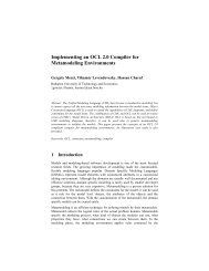
To calculate oscillator signal z d trapezoidal integration routine was used. In addition
to ensure numerical stability of the algorithm scaling operation was performed to
stabilized envelope of ‖z d ‖ determined by function δ d (t).
Figure 7: Controller diagram
Remark 6 It should be noted that implemented control scheme is based on assumption
that longitudinal slip is negligible. In theory this assumption would not be
necessary for overall controller previously verified in simulation section.
5.2 Results
To validate the proposed simplified algorithm results of experiments are presented.
Firstly, we considered the regulation problem, i.e. parking problem. The parameters
of the controller and initial conditions were presented in section 4, however ε 1 was
increased to 0.05 to ensure better robustness and less sensitiveness to measurement
noise.
The results are depicted in Figs. 7(a)–7(b). From Fig. 7(a) one can see that steadystates
position and orientation errors were bounded as follows
∣ ˜X
∣
∣
∣ < 20[mm], ∣Ỹ ∣ < 20[mm], ∣˜θ ∣ < 0.03[rad].
In the next experiment trajectory tracking was verified. The reference trajectory was
the same as it used in simulation and the parameter ε 1 was selected as ε 1 = 0.15
to improve robustness of the controller. From Fig. 8(a) and 8(b) one can see that
accuracy of tracking is significantly less than accuracy obtained for regulation that
results mainly from unmodeled dynamic effects (for example slip phenomenon) and
delays in the control loop. The tracking errors were bounded as
∣ ˜X
∣ < 80[mm],
∣
∣Ỹ
∣ < 180[mm],
∣
∣˜θ ∣ < 0.3[rad].

Y [m]
0.6
0.5
0.4
0.3
0.2
0.1
0
q(t)
q r
(t)
q(0)
q r
(0)
−0.1
−0.4 −0.2 0 0.2 0.4
X [m]
Y [m]
0.6
0.4
0.2
0
−0.2
(a) Performed trajectory
X−X r
, Y−Y r
[m]; θ−θ r
[rad]
1
0.5
0
−0.5
−1
−1.5
−2
X−X r
Y−Y r
θ−θ r
−2.5
0 5 10 15 20 25 30
time [s]
(b) Regulation errors
Figure 8: Experimental results – regulation case
q(t)
q r
(t)
q(0)
q r
(0)
−0.4
0 0.5 1 1.5
X [m]
(a) Performed and reference trajectory
X−X r
, Y−Y r
[m]; θ−θ r
[rad]
0.4
0.2
0
−0.2
X−X r
−0.4
Y−Y r
θ−θ r
−0.6
0 5 10 15
time [s]
(b) Tracking errors
Figure 9: Experimental results – trajectory tracking case
6 Summary
In this paper the control algorithm which resolves both trajectory tracking and regulation
problem for 4-wheel skid-steering mobile robot is presented. In particular
much attention is dedicated to show implementation and experimental results for
the controller. We believe that further improvement of accuracy is possible by using
a new measurement and localization system in form of monolithic optical sensors
and accelerometers. It would allow to implement overall control scheme presented
in theoretical description.
On the other hand it is worthy to note that SSMR is quite difficult to control that
results from unmodeled dynamic effects, hence achieving small tracking errors may
be impossible. Therefore the algorithms which ensure practical stabilization with
good robustness on unmodeled phenomena can be very useful in practice [8].

References
[1] R. W. Brockett, “Asymptotic stability and feedback stabilization”, Differential Geometric
Control Theory edited by R. W. Brockett, R. S. Milman and H. J. Susmann,
Birkhauser, Boston, pp. 181-191, 1983.
[2] L. Caracciolo, A. De Luca, S. Iannitti, “Trajectory tracking control of a four-wheel differentially
driven mobile robot”, IEEE Int. Conf. on Robotics and Automation, Detroit,
MI, pp. 2632-2638, May 1999.
[3] G. Campion, G. Bastin, B. DAndrea-Novel, “Structural Properties and Classification of
Kinematic and Dynamic Models of Wheeled Mobile Robots”, IEEE Transactions on
Robotics and Automation, Vol. 12, No.1, pp. 47-62, February 1996.
[4] W.E.Dixon, A.Behal, D.M.Dawson, S.P.Nagarkatti, Nonlinear Control of Engineering
Systems, A Lyapunov-Based Approach, Birkhauser 2003.
[5] W. E. Dixon, D. M. Dawson, E. Zergeroglu and A. Behal, Nonlinear Control of
Wheeled Mobile Robots, Springer-Verlag, 2001.
[6] P. Dutkiewicz, M. Kiełczewski, “Vision feedback in control of a group of mobile
robots”. Proc. of the Seventh International Conference on Climbing and Walking
Robots and their Supporting Technologies for Mobile Machines CLAWAR 2004, Madrit
2004 (to appear).
[7] P. Morin, C. Samson, “Practical Stabilization of Driftless Systems on Lie Groups: The
Transverse Function Approach”, IEEE Transactions on Automatic Control, Vol. 48,
No.9, pp.1496-1508, September 2003.
[8] P. Morin, C. Samson, “Feedback control of nonholonomic wheeled vehicles, A survey”,
Archives of Control Sciences, Vol. 12, pp.7-36, 2002.
[9] T. Jedwabny, M. Kowalski, M. Kiełczewski, M. Ławniczak, M. Michalski,
M. Michałek, D. Pazderski, K. Kozłowski, Nonholonomic mobile robot MiniTracker 3
for research and educational purposes, 35 th International Symposium on Robotics,
Paris 2004.
[10] K. Kozłowski, D. Pazderski, “Control of a Four-Wheel Vehicle Using Kinematic Oscillator”.
Proc. of the Sixth International Conference on Climbing and Walking Robots
and their Supporting Technologies CLAWAR 2003, pp. 135-146, Catania 2003.
[11] H. B. Pacejka, Tyre and Vehicle Dynamics, Butterworth-Heinemann, 2002.
[12] D. Pazderski, K. Kozłowski, M. Ławniczak, “Practical stabilization of 4WD skidsteering
mobile robot”. Proc. of the Fourth International Workshop on Robot Motion
and Control, Puszczykowo, pp. 175-180, 2004.
[13] D.Pazderski, K.Kozłowski, W.E.Dixon, “Tracking and Regulation Control of a Skid
Steering Vehicle”, American Nuclear Society Tenth International Topical Meeting on
Robotics and Remote Systems, Gainesville, Florida, pp. 369-376, March 28-April 1
2004.
[14] M. W. Spong, “On the Robust Control of Robot Manipulators”, IEEE Transactions on
Automatic Control, Volume 37, No. 11, pp. 1782-1786, November 1992.