Lecture Notes Discrete Optimization - Applied Mathematics

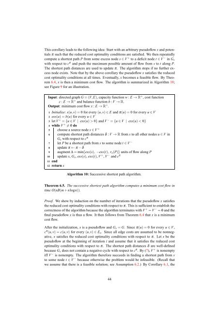
This corollary leads to the following idea: Start with an arbitrary pseudoflow x and potentials
π such that the reduced cost optimality conditions are satisfied. We then repeatedly
compute a shortest path P from some excess node s∈ V + to a deficit node t ∈ V − in G x
with respect to c π and push the maximum possible amount of flow from s to t along P.
The shortest path distances are used to update π. The algorithm stops if no further excess
node exists. Note that by the above corollary the pseudoflow x satisfies the reduced
cost optimality conditions at all times. Eventually, x becomes a feasible flow. By Theorem
6.4, x is then a minimum cost flow. The algorithm is summarized in Algorithm 10;
see Figure 9 for an illustration.
Input: directed graph G=(V,E), capacity function w : E →R + , cost function
c : E →R + and balance function b : V →R.
Output: minimum cost flow x : E →R + .
1 Initialize: x(u,v)=0 for every(u,v)∈E and π(u)= 0 for every u∈ V
2 exs(u)=b(u) for every u∈ V
3 let V + ={u∈ V | exs(u)>0} and V − ={u∈ V | exs(u)