
Create successful ePaper yourself
Turn your PDF publications into a flip-book with our unique Google optimized e-Paper software.
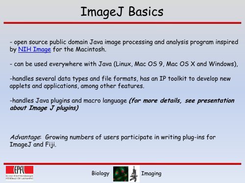
<strong>ImageJ</strong> <strong>Basics</strong><br />
- open source public domain Java image processing and analysis program inspired<br />
by NIH Image for the Macintosh.<br />
- can be used everywhere with Java (Linux, Mac OS 9, Mac OS X and Windows),<br />
-handles several data types and file formats, has an IP toolkit to develop new<br />
applets and applications, among other features.<br />
-handles Java plugins and macro language (for more details, see presentation<br />
about Image J plugins)<br />
Advantage: Growing numbers of users participate in writing plug-ins for<br />
<strong>ImageJ</strong> and Fiji.<br />
Biology<br />
Imaging
Index<br />
-Installing <strong>ImageJ</strong> (windows) and plugins p. 3 - 4<br />
-Memory settings p. 5<br />
-Menu and Tools overview p. 6<br />
-File menu: Opening, importing, saving files p. 7 - 8<br />
-Image menu and Image types p. 9 - 11<br />
-Image visualisation/information p. 12<br />
RGB channel splitting/merging/overlays p. 13<br />
Stacks p. 14 – 15<br />
-Image Adjustments<br />
Brightness/Contrast p. 16<br />
Threshold p. 17<br />
Image Crop/Transform/Rotate/Revert p. 18<br />
-Image quantification<br />
Calibrating image size/ Scale bars p. 19<br />
Histogram and line profile p. 20<br />
<strong>ImageJ</strong> Region measurements p. 21-22<br />
Biology<br />
Imaging
Installation<br />
Different editions of <strong>ImageJ</strong> exist:<br />
32bit and 64bit<br />
1. Image J homepage for software and plugin downloads:<br />
http://rsbweb.nih.gov/ij/<br />
Wiki: http://imagejdocu.tudor.lu/<br />
Must have java.exe installed to run <strong>ImageJ</strong> (available with IJ)<br />
2. For a version with pre-installed plugins:<br />
The MBF <strong>ImageJ</strong> collection of plugins and macros<br />
http://www.macbiophotonics.ca/imagej/installing_imagej.htm<br />
3. Fiji is a similar software based on <strong>ImageJ</strong>:<br />
http://pacific.mpi-cbg.de/wiki/index.php/Main_Page<br />
Obtaining Image J Version information and updating the software:<br />
> Help > About <strong>ImageJ</strong> - version information<br />
> Help > Update <strong>ImageJ</strong><br />
Biology<br />
Imaging
Plugins & Macros<br />
Plugins are additional software modules or code which provide the ability to perform<br />
specific tasks. Writing macros using the <strong>ImageJ</strong> macro language allows you to<br />
string a series of commands together to perform batch operations. These can also be<br />
converted to plugins.<br />
‣Install plugins if required:<br />
Download plugins and Save them in <strong>ImageJ</strong> Plugin folder (program files)<br />
Restart <strong>ImageJ</strong>: Plugins automatically get placed in the Plugins menu<br />
> There is a list of available plugins here:<br />
http://rsb.info.nih.gov/ij/plugins/index.html<br />
> There is a plugins collection preorganised in folders available at:<br />
http://rsb.info.nih.gov/ij/plugins/collection.html<br />
> Many more are available on the website and from other users. Some people have<br />
developed their own collections of plugins and bundled them together. McMaster<br />
Biophotonics Institute has a great collection for microscopy:<br />
http://rsb.info.nih.gov/ij/plugins/mbf-collection.html<br />
Biology<br />
Imaging
<strong>ImageJ</strong> memory<br />
‣Set high memory for optimal use<br />
no more than 70% of max Ram<br />
‣Edit > Options > Memory<br />
Biology<br />
Imaging
<strong>ImageJ</strong> menus and tool bars<br />
Menu bar<br />
(Biophotonics edition)<br />
Tool bar<br />
Status bar<br />
Region/Measurement tools<br />
Image visualisation<br />
and adjustments<br />
Switch to alternative Tool bar themes.<br />
Very useful in original <strong>ImageJ</strong>.<br />
Biophotonics edition (shown here) already<br />
starts up with a useful Tool bar.<br />
Biology<br />
Imaging
File menu: Opening, importing, saving files<br />
‣ Drag and drop file to <strong>ImageJ</strong> menubar to open file<br />
‣ Open<br />
microscope image formats: .lei .lsm<br />
many image and video formats: .avi .tif<br />
‣ Import<br />
-image sequence…<br />
Open and manage stacks/movies<br />
-many file types and text files/results<br />
‣ Save movies as .avi as compressed<br />
jpeg<br />
Drastically reduces file size without<br />
quality loss (for presentations for ex.)<br />
‣ Save images as .tif<br />
A JPEG image degrades each time it<br />
is opened, edited and resaved.<br />
Biology<br />
Imaging
Importing OME BIO LOCI & metadata<br />
http://www.loci.wisc.edu/software/bio- formats<br />
informs you on types of compatible formats<br />
‣ Open Bio-formats Importer Plugin<br />
-to import a wide range of formats<br />
-to select meta data to display<br />
Biology<br />
Imaging
Image Menu<br />
Working with different image types and adjustments can be accessed via the Image Menu<br />
or via image adjustment buttons on the second half of the tool bar<br />
Biology<br />
Imaging
Image type: 8, 16 bit, RGB<br />
Binary image:<br />
For this type of code, each pixel is either black or white because one bit can<br />
code for one pixel (0 = black, 1 = white).<br />
1 pixel = 1 bit of memory<br />
Image in gray levels: 8bit or 16bit<br />
If we code each pixel on 2 bits we would have 2 2 = 4 possibilities (black, dark<br />
gray, light gray, white). But this image would have very limited levels.<br />
So in general we use 8 or 16bits:<br />
2 8 = 256 possibilities (0 - 255 grey levels) 8 bits = 1 octet (1 byte)<br />
2 16 = 4096 possibilities (0 - 4095 grey levels) 16 bits = 2 octets<br />
Multiply number of pixels by number of bits to get memory:<br />
8 bit image: 1000 pixels = 1000 octets = 1 kbyte<br />
Quantification requires 16bit images (bigger window)<br />
Tif images don’t have 12 bit (usually converted to 16)<br />
Acquisition detectors usually only detect in 12 bit!<br />
Biology<br />
Imaging
Image type: greyscale LUTs, RGB<br />
‣Pseudocolour in greyscale:<br />
8bit and 12bit greyscale images can be visualised in colour:<br />
Use LookUp tables (LUTs): Assigns a range of colour to the grey levels<br />
> Either use LUT button on startup tool bar or switch to LUT tool bar by<br />
pressing on<br />
(Biophotonics edition)<br />
The following tool bar appears:<br />
‣Colour image (RGB):<br />
an overlap of 3 pixels 8bit (24 bit total)<br />
It’s an additive principle of colours:<br />
We can obtain a certain colour by adding 3 primary colours in various<br />
proportions: 256x256x256 = more than 16 million colours.<br />
Different type of colour coding: RGB, CYMK.<br />
RGB: each colour is coded on 1 octet (8bits). Each pixel is a combination of 3<br />
octets (3 x 8 = 24 bits total with Red = 0-255, Green = 0-255, Blue = 0-255.<br />
1 pixel = 3 octets = 24 bits<br />
Biology<br />
Imaging
Image information & Visualisation<br />
Status Bar = information for cursor<br />
position (x,y) and intensity value.<br />
Or memory usage<br />
Top of Image = information:<br />
Channels<br />
Image size (um or pixels)<br />
Image type (bits)<br />
Image memory<br />
Depending on image dimensions,<br />
Scroll bars appear at the bottom<br />
to scroll across<br />
c: channels<br />
z: stack slices<br />
t: time frames<br />
Biology<br />
Imaging
RGB channel splitting/merging/overlays<br />
‣Image > Color > Merge (overlay)/Split channels<br />
Press once: Merges channels of an RGB stack to one RGB file<br />
Press twice: Splits into 3 individual channels<br />
Press again: Merges channels back with options as to which channel goes where. Overlay<br />
possible with transmitted light images by using the Gray channel. Do not create<br />
composite.<br />
Biology<br />
Imaging
Stacks…<br />
‣Image > Stacks<br />
You need to have a series (time, z, x-y) of images which can be built into a stack. Opeining<br />
images as a numbered sequence will automatically create a stack.<br />
Compatible with Metamorph stacks.<br />
Measuring and analysis tools can be often used to apply to all images in a stack<br />
Convert Images to Stack: converts a set of 2D images that you have opened into a stack.<br />
Animate: animates the images in a stack at a rate up to 100 frames per second.<br />
Convert Stack to Images: splits the stack into individual images.<br />
Next Slice/Previous Slice: browsing images can be done using the > and < keys. The<br />
number of the current slice and the total number of slices are displayed in the title bar.<br />
You can also use the slider bar in the stack window.<br />
Z Project: simple projection algorithms designed to render 3D images into 2D<br />
projections, allows volume rendering, useful for visualizing the internal structures of 3D<br />
images.<br />
Biology<br />
Imaging
…Stacks<br />
For immediate maximum intensity projection (MIP) use this button on the tool bar:<br />
‣Image > Stack > 3D Project: Allows you to project the stack and then rotate it.<br />
‣Orthogonal view: provides an orthogonal (or section) view.<br />
‣Image > Duplicate allows you to save the slice you are viewing as an individual file<br />
‣Image > Stacks > Movies<br />
Time stamper: allows you to add the time information onto your movie.<br />
Zoomify: allows you to make a movie where you zoom in on a particular region.<br />
Biology<br />
Imaging
Image Adjustments: Brightness/Contrast<br />
‣Image Adjust > Brightness/Contrast<br />
Or B/C Button on tool bar<br />
Contrast and brightness: use to enhance<br />
images by dynamically changing the lookup<br />
table mapping.<br />
Click on the brightness slider and drag from<br />
side to side.<br />
You can also adjust the contrast setting<br />
independently.<br />
Brightness - adds or subtracts a constant to<br />
each pixel – shift in histogram along x axis<br />
but doesn’t change the<br />
distribution.<br />
Contrast – lower level set (e.g. to 0) and<br />
higher level set (e.g. to 255) and rest of pixel<br />
values adjusted<br />
proportionally.<br />
Biology<br />
DO NOT CLICK on APPLY. This stretches<br />
the histogram to fit new min and max values<br />
and is not reversible. This affects future<br />
Measurements!<br />
Imaging
Image Adjustments: Threshold<br />
‣Image > Adjust >Threshold<br />
is the simplest method of image<br />
segmentation. From a grayscale<br />
image, thresholding can be used to<br />
create binary images.<br />
Threshold above/below: Individual<br />
pixels in an image are marked as<br />
“object” pixels if their value is<br />
greater/lower than some threshold<br />
value (assuming an object to be<br />
brighter than the background) and<br />
as “background” pixels otherwise.<br />
Threshold inside/outside, when a<br />
pixel value is between two<br />
thresholds/vice-versa.<br />
Typically, an object pixel is given a value of “1” while a background pixel is given a value of<br />
“0.” Finally, a binary image is created by coloring each pixel white or black, depending on a<br />
pixel's label.<br />
Wikipedia<br />
Biology<br />
Imaging
Image Crop/Transform/Rotate/Revert<br />
‣Image ><br />
Crop - You can make selection areas to determine the area to be cropped<br />
Rotate - You can also Rotate the image into different angles<br />
All this can be applied to a single image or to all slices of a stack<br />
‣File > Revert<br />
And revert to the original file (File > Revert or Control-R)<br />
To be safe, always click on Image > Duplicate and work on the copy of your image<br />
Biology<br />
Imaging
Calibrating image size units<br />
Calibrating image size is important<br />
for further image processing:<br />
-measurements<br />
-scale bar<br />
‣ Image > Properties<br />
Enter unit of length ( m or pixels)<br />
Image now shows image size in m<br />
‣ Press scale bar button in tool menu<br />
to add scale bar to single image or all<br />
slices of a stack.<br />
Biology<br />
Imaging
Image histogram and line profile<br />
Histogram:<br />
Shows the number of pixels of<br />
each value, regardless of location, and the mean<br />
and max values. The log display allows for the<br />
visualization of minor components.<br />
‣ Analyse > Histogram<br />
‣ Generate list of values by<br />
clicking on List.<br />
Line plot: Shows the intensity profile of<br />
pixels along a selection.<br />
Select line tool, draw line for profiling<br />
‣ Analyse > Plot profile<br />
Biology<br />
Imaging
<strong>ImageJ</strong> Region measurements<br />
‣ Area SelectionTools<br />
-Use these tools to create area selections -Location, width and height are displayed in<br />
the status bar. (Change properties of selection regions in Edit > Selection > Properties<br />
-The contents of an region can be copied, cleared (to white), filled with the current<br />
drawing color, outlined (using Edit/Draw), filtered, or measured.<br />
Backspace<br />
- Edit/Clear<br />
> Image > Colors -Set the drawing color<br />
Double click any line tool<br />
- Change the line width used by Edit/Draw<br />
Arrow keys with ALT<br />
- to "nudge" a selection one pixel at a time<br />
Use the small "handles"<br />
- to resize<br />
Holding down Alt<br />
- forces ellipse circles or rectangles squares<br />
-To create the polygonal selection, click repeatedly with the mouse to create line<br />
segments, double click when finish.<br />
-Use the wand tool to reposition selections drawn with the rectangle capture tool, oval<br />
capture tool, etc.<br />
Biology<br />
Imaging
<strong>ImageJ</strong> Region measurements<br />
‣Measurements can be<br />
managed and logged through<br />
the Region of Interest (ROI)<br />
Manager available in the<br />
Biophotonics <strong>ImageJ</strong><br />
Version tool bar, or from<br />
‣Image > Analysis > Tools<br />
Create regions with the selection tools<br />
Click on Add or type t<br />
Select Show All so that the regions appear visible<br />
Go to More > and choose Measure all<br />
‣In Analyse > Set Measurements: you can decide<br />
What type of measurements will appear in the list.<br />
You can save the region measurements (More > Save)<br />
And apply them to all stacks or to new images<br />
You can also save the results as an excel file.<br />
Biology<br />
Imaging