Use of the GFDL Vortex Tracker - DTC

Use
of
the
GFDL
Vortex
Tracker
Tim
Marchok
NOAA
/
Geophysical
Fluid
Dynamics
Laboratory
WRF
Tutorial
for
Hurricanes
February
25,
2010

Outline
• History
&
descripKon
of
the
GFDL
vortex
tracker
• Inputs
&
Outputs
• ATCF‐plot:

GrADS‐based
track
and
intensity
ploRng
script

GFDL
Vortex
Tracker:

History
• Requirements:
A
flexible
tracking
algorithm
to
work
on
a
variety
of
models
and
resoluKons.
Must
run
quickly
Must
produce
output
in
ATCF
format
• Became
operaKonal
at
NCEP
in
1998

Purpose
of
a
vortex
tracker
.
.
11000100100100101010
00010010011110010010
11001110001101010001
00001010010011001011
10101110101100011001
10001110100100010100
.
.
NOW
WHAT
?
• OperaKons:
Quick
reporKng
of
track
and
intensity
forecast
data
to
NHC,
JTWC,
others.
• Research:

Quick
evaluaKon
of
the
track
&
intensity
skill
of
a
forecast

Why
the
need
for
an
external
tracker?
• Valuable
CPU
Kme
is
not
wasted
during
model
execuKon.
• Tracking
analysis
can
be
re‐done
without
rerunning
model.
• Uniform
tracking
criteria
can
be
applied
to
mulKple
models.

Why
the
need
for
an
external
tracker?
• Ike
in
HWRF:
A
well‐defined
storm
with
center
locaKons
collocated.
• So
then…
why
the
need
for
anything
sophisKcated?

Why
the
need
for
an
external
tracker?
• Gustav
in
GFS:
For
an
observed
80‐knot
hurricane,
the
GFS
was
iniKalized
with
a
poorly
organized
vorKcity
center.

Why
the
need
for
an
external
tracker?
• Gustav
in
GFS:
The
SLP
center
was
found
188
km
from
the
vorKcity
center.


What
is
the
storm’s
central
posi1on?

Why
the
need
for
an
external
tracker?
Also
note:

The
center
locaKons
for
the
parameters
were
not
found
exactly
at
a
model
gridpoint
• Gustav
in
GFS:
The
SLP
center
was
found
188
km
from
the
vorKcity
center.

Tracker
Design:


MulKple
Variables
• A
weighted
average
of
the
posiKons
of
several
low‐level
variables
is
used.
• 6
Primary
parameters:
850
mb
vorKcity
700
mb
vorKcity
Surface
(10
m)
vorKcity
850
mb
gp
height
700
mb
gp
height
Mean
Sea‐Level
Pressure
• 3
Secondary
parameters:
850
mb
minimum
in
wind
speed
700
mb
minimum
in
wind
speed
Surface
(10
m)
minimum
in
wind
speed

Tracker
Design:


Center‐fixing
algorithm
• Instead
of
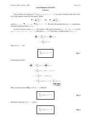
interpolaKon,
a
Barnes
Analysis
is
performed
on
an
array
of
points
surrounding
a
guess
storm
locaKon:
The
Barnes
funcKon,
B,
provides
a
Gaussian‐weighted
average
value
for
a
variable,
F(n),
at
a
given
gridpoint,
g.
The
weighKng
funcKon,
w,
is
dependent
on
the
distance,
d n ,
of
a
point
from
the
origin
gridpoint,
g,
and
the
choice
of
the
e‐folding
radius,
r e .
The
center
is
found
at
the
point
where
this
Barnes
funcKon
is
maximized
(e.g.,
NH
vorKcity)
or
minimized
(e.g.,
MSLP).

Barnes
analysis
weighKng
Linear
Response
SpaKal
Response
Grid spacing = 0.1 o
Latitude
Longitude
• Choosing

r e :

A
balance
between
including
enough
points
to
get
a
representaKve
sample
vs.
too
much
smoothing.
• For
most
models,
we
use
r e 
=
75
km.

For
dx

Barnes
analysis:
mulKple
search
iteraKons
NHC
observaKons
indicate
a
storm
iniKally
located
here
Model
data
grid
Latitude
Longitude

Barnes
analysis:
mulKple
search
iteraKons
Model
data
grid
+
Barnes
analysis
grid
A
grid
of
analysis
points
is
set
up,
relaKve
to
the
NHC
observed
posiKon.
Latitude
A
Barnes
analysis
is
performed
for
all
points
within
a
specified
distance
from
the
NHC
posiKon.
Longitude Latitude

Barnes
analysis:
mulKple
search
iteraKons
Aker
the
first
iteraKon
through
all
the
points,
suppose
the
Barnes
analysis
idenKfies
the
center
as
being
here.
Model
data
grid
+
Barnes
analysis
grid
Latitude
Longitude Latitude

Barnes
analysis:
mulKple
search
iteraKons
Model
data
grid
+
Barnes
analysis
grid
A
second
iteraKon
through
the
Barnes
analysis
is
performed
aker
further
limiKng
the
domain
and
halving
the
grid
spacing.
Latitude
Longitude

Barnes
analysis:
mulKple
search
iteraKons
This
process
is
repeated
mulKple
Kmes
(up
to
5),
halving
the
grid
spacing
for
the
Barnes
analysis
each
Kme,
unKl
a
center
posiKon
is
fixed
using
a
Barnes
analysis
grid
spacing

CompuKng
the
center
posiKon,
Part
I
The
Barnes
analysis
is
repeated
for
all
6
primary
parameters
to
produce
fix
posiKons
for
each.
Model
data
grid
2
5
3
 4
 1
 6
Parameters
fixes
that
are
within
a
specified
error
distance
threshold
of
the
current
guess
posiKon
are
used
to
create
a
preliminary
mean
fix.
Latitude
Longitude

CompuKng
the
center
posiKon,
Part
II
The
Barnes
analysis
is
repeated
for
the
3
secondary,
windbased
parameters.
Model
data
grid
This
analysis
is
performed
over
a
small
domain,
centered
on
a
posiKon
that
is
a
mean
of
the
6
primary
fixes
and
the
guess
posiKon.
Latitude
Longitude

CompuKng
the
center
posiKon,
Part
III
Parameters
fixes
that
are
beyond
a
specified
error
distance
threshold
of
the
current
guess
posiKon
are
discarded.
• Error
distance
thresholds:
IniKally
275
km
At
later
Kmes,
can
be
a
funcKon
of
spread
in
previous
posiKon
fixes
Latitude
Model
data
grid
2
5
 7
3
 4
 9
1
 8
 6
Longitude

CompuKng
the
center
posiKon,
Part
III
The
remaining
Model
data
grid
parameter
fixes
are
averaged
to
produce
the
mean
posiKon
fix
+
for
each
forecast
hour.
• These
addiKonal
parameters
are
computed
once
the
center
fix
is
made:
Max
surface
wind
Latitude
R max
Minimum
MSLP
34‐,
50‐
and
64‐kt
wind
radii
Longitude

Tracking
from
one
lead
Kme
to
the
next
Linear
extrapolaKon
Barnes
analysis
&
advecKon
+
t‐1
+
t
t+1
Latitude
Longitude
The
guess
posiKons
from
these
2
methods
are
averaged
to
compute
a
final
guess
posiKon
for
the
search
at
the
next
lead
Kme.
A
Barnes
analysis
with
a
large
r e
at
850,
700
&
500
mb
is
used
to
compute
mean
steering
winds.
A
parcel
is
advected
to
a
guess
posiKon
at
the
next
lead
Kme.

“Quality
Control”
A
series
of
checks
is
applied
to
ensure
that
the
tracker
is
following
a
storm
that
is
the
system
of
interest
MSLP
Gradient:

Gross
check
to
ensure
minimum
gradient
(~0.5
mb
/
300
km)
exists
within
300
km
of
center.

Set
in
script:
“mslpthresh”
variable
DIST (MSLP‐Zeta850) :

This
distance
between
the
MSLP
and
Zeta 850
parameter
fixes
must
not
exceed
a
distance
defined
in
source
by
“max_mslp_850”
(usually
set
to
323
km).
V T 
(850
mb):

Mean
V T 
within
225
km
must
be
cyclonic
and
exceed
threshold.

Default
(1.5
ms ‐1 )
is
set
in
script:
“v850thresh”
variable
Transla?onal
speed:

Speed
of
storm
movement
must
not
exceed
threshold,
set
by
“maxspeed_tc”
variable
(usually
set
to
60
knots).

Outline
• History
&
descripKon
of
the
GFDL
vortex
tracker
• Inputs
&
Outputs
• ATCF‐plot:

GrADS‐based
track
and
intensity
ploRng
script

Tracker
inputs:

SynopKc
data
• Data
must
be
in
Gridded
Binary
(GRIB)
Version
1
format.
• Data
points
must
increment
from
northwest
(1,1)
to
southeast
(imax,
jmax).
• Data
must
be
on
a
lat/lon
grid.
• dx
does
not
need
to
equal
dy,
but
both
must
remain
uniform
over
the
domain.
(1,1)
(imax,jmax)
• Data
lead
Kme
intervals
do
not
need
to
be
evenly
spaced

Tracker
inputs:

Observed
TC
data
• Tracker
searches
for
a
vortex
iniKally
at
a
locaKon
specified
by
NHC
or
JTWC
on
a
“TC
Vitals
record”:
NHC

12L
KATRINA


20050829
0000
272N
0891W
335
046
0904
1006
0649
72
037
0371
0334
0278
0334
D
0204
0185
0139
0185
72
410N

815W
0167
0167
0093
ATCF

ID
(12L
=
12 th
storm
in
the
AtlanKc).
E
=
Eastern
Pacific
C
=
Central
Pacific
W
=
Western
Pacific
Report
date
and
Kme
Observed
storm
laKtude
&
longitude
Observed
direcKon
of
storm
moKon
in
degrees
from
north
(335
=
~NNW),
and
storm
translaKon
speed
(046
=
4.6
ms ‐1 )

Tracker
inputs:

Namelist
opKons
Starting date & time
ID number for model in the executable. Leave as ‘17’
Indicator for GRIB data lead time units
Obsolete, leave as ‘83’
ATCF model name: “HWRF”, “HAHW”, “TEST”, etc
Starting yyyymmddhh for output ATCF record
For genesis tracking use. Fill with any values, as shown.
‘tracker’, ‘midlat’, ‘tcgen’. Only use ‘tracker’ here
Thresholds for mslp gradient and V 850
Model grid type: ‘regional’ or ‘global’
Not yet supported. Leave values as they are….

Tracker
inputs:

List
of
forecast
hours
• The
tracker
can
handle
lead
Kmes
that
are
stored
in
the
GRIB
file
header
either
in
units
of
minutes
or
hours.
• Explicitly
detailing
the
forecast
hours
allows
for
irregularly
spaced
intervals.
• Regardless
of
whether
your
GRIB
data
lead
Kme
units
are
in
minutes
or
hours,
you
must
supply
a
text
file
as
input
that
has
the
lead
Kmes
listed
in
minutes
(code
will
convert
to
hours).

Tracker
output:

Standard
ATCF
file
• Text
format.

Minimum
of
1
record
per
lead
Kme
(

),
maximum
of
3.
1 st 
record
contains
track
&
intensity
info,
plus
radii
for
34‐
knots
winds
2 nd 
record:

Same
track
&
intensity
info,
plus
radii
for
50‐
knot
winds,
if
present.
3rd
record:

Same
track
&
intensity
info,
plus
radii
for
64‐
knot
winds,
if
present.

Tracker
output:

Standard
ATCF
file

Tracker
output:

Modified
ATCF
file
• Nearly
same
format
as
standard
ATCF
file,
except
the
lead
Kme
(

)
has
2
extra
places
for
fracKon
of
an
hour,
allowing
for
ATCF‐style
output
at
non‐hourly
Kmes.
Example:

“04825”
would
be
48.25
hours,
or
48
hours,
15
minutes.

Tracker
output:

Standard
out
• A
table
is
printed
out
that
lists
the
tracker‐derived
fixes
for
each
parameter
and
distance
from
the
guess.
Maximum allowable distance that a parameter fix can be
from the guess location in order to be included
Storm & lead time info
Guess
location for
this lead
time
Max or min
barnes-averaged
value found by
tracker
Distance of
parameter fix
from guess
location
Flag to indicate if parameter fix is within errmax distance and
will be included in fix average for this lead time

Outline
• History
&
descripKon
of
the
GFDL
vortex
tracker
• Inputs
&
Outputs
• ATCF‐plot:

GrADS‐based
track
and
intensity
ploRng
script

ATCF_plot:

GrADS‐based
ploRng
tool
• InteracKve
GrADS
tool
for
ploRng
both
track
and
intensity.

ATCF_plot:

How
it
works
atcfplot.gs
User‐input
selecKons
for
models,
storm,
date,
etc,
are
passed
to
unix
scripts.
Unix
scripts
The
unix
scripts
pull
only
the
requested
ATCF
records
from
the
ATCF

file
for
the
user‐selected
storm…
.
.
aal072008.dat
aal082008.dat
aal092008.dat
aal102008.dat
.
.
aal172008.dat
The
ATCF
records
from
those
flist
and
vlist
text
files
are
read
by
atcfplot.gs,
and
the
track
and
intensity
plots
are
created.
flist
vlist
…and
dumps
those
ATCF
records

into
text
files.

ATCF_plot:

Script
setup
• Edit
path
names
to
replace
$USER
with
your
username
in
your
version
of
atcfplot.gs:
_rundir="/wrfclass/users/$USER/HWRF/src/gfdl‐vortextracker/trk_plot/plovrak/"
_netdir="/wrfclass/users/$USER/HWRF/src/gfdl‐vortextracker/trk_plot/plovrak/tracks/“
• For
all
atcfplot
unix
scripts
here
at
the
tutorial,
all
paths
are
defined
using
environmental
variables
$HOME
and
$USER.

Back
at
home,
be
sure
to
change
the
path
names
accordingly.

ATCF_plot:

Input
data
• atcf_plot
reads
in
standard
ATCF
format
records,
but
it
needs
the
opera1onal
ATCF
files,
since
it
keys
off
of
the
observaKonal
“CARQ”
records
and
uses
that
data
to
plot
the
observed
track
and
intensity
(note:
Real‐Kme
data
used,
not
Best
Track).
• Be
sure
to
insert
your
ATCF
records
in
the
ATCF
file
specifically
named
a${basin}${storm_ID}${YYYY}.dat
aker
the
CARQ
records
for
the
correct
DTG:

ATCF_plot:

Input
data
• atcf_plot
opens
up
a
GrADS
ctl
file
(plovrak.ctl)
that
points
to
a
meaningless
data
set
with
a
global
domain.

By
opening
this
ctl
file
and
ploRng
a
variable,
GrADS
now
has
global
dimensions
over
which
we
can
plot
tracks
for
TCs
anywhere
on
the
globe.
• Be
sure
to
also
have
the
plovrak.grib
file,
then
from
your
unix
prompt
run
the
command
“gribmap
–v
–i
plovrak.ctl”.

In
the
output,
you
should
see
one
line
that
says
“MATCH”.
• To
run,
enter
this
command
from
your
unix
prompt:
atcfplot.sh

YYYY

basin
where
basin
=
al,
ep,
wp,
etc….

ATCF_plot:

Some
features
• Plot
tracks
alone,
intensity
alone,
or
tracks
with
an
intensity
inset
window.
• Plot
tracks
that
span
from
the
current
DTG
through
the
end
of
the
storm’s
lifecycle
• The
ability
to
click
&
drag
to
zoom
in
on
a
parKcular
track
segment.

QuesKons?
Delaware River flooding River Road in
Washington Crossing, Pennsylvania,
after Hurricane Ivan. September, 2004.