Simulations of Biomolecules Using Molecular Dynamics
Simulations of Biomolecules Using Molecular Dynamics
Simulations of Biomolecules Using Molecular Dynamics

You also want an ePaper? Increase the reach of your titles
YUMPU automatically turns print PDFs into web optimized ePapers that Google loves.
Chemistry 380.37<br />
Fall 2011<br />
Dr. Jean M. Standard<br />
November 30, 2011<br />
<strong>Simulations</strong> <strong>of</strong> <strong>Biomolecules</strong> <strong>Using</strong> <strong>Molecular</strong> <strong>Dynamics</strong><br />
Introduction<br />
The first molecular dynamics simulation <strong>of</strong> a biomolecule was a simulation <strong>of</strong> bovine pancreatic trypsin inhibitor<br />
(BPTI) in 1977 [J. A. McCammon, B. R. Gelin, and M. Karplus, Nature 267, 585 (1977)]. BPTI was chosen for<br />
simulation because it is relatively small (58 residues) and a high-resolution x-ray crystal structure was available at<br />
the time (Figure 1). The simulation was carried out in vacuum and was 9.2 ps in length.<br />
Figure 1. Atomic model and ribbon diagram <strong>of</strong> BPTI.<br />
Eleven years later, a molecular dynamics simulation <strong>of</strong> BPTI was carried out in solution [M. Levitt and R. Sharon,<br />
Proc. Nat. Acad. Sci. 85, 7557 (1988)]. This simulation, including water molecules, consisted <strong>of</strong> approximately<br />
8700 atoms (892 protein atoms and 7821 solvent atoms) and was 210 ps in length with a step size <strong>of</strong> 2 fs. The<br />
force fields employed in these early gas and solution phase simulations were quite crude compared to those employed<br />
in similar simulations today.<br />
Thanks to the enormous increase in computing power over the last 10 years, biomolecular simulations today can be<br />
performed on systems <strong>of</strong> hundreds <strong>of</strong> thousands <strong>of</strong> atoms and for times on the order <strong>of</strong> nanoseconds (some<br />
approaching microseconds). <strong>Molecular</strong> dynamics simulations may be employed to study a wide variety <strong>of</strong><br />
behaviors <strong>of</strong> biomolecules, from the dynamics <strong>of</strong> binding <strong>of</strong> carbon monoxide to hemoglobin to the mechanism <strong>of</strong><br />
the passage <strong>of</strong> ions through the gramicidin A ion channel. An excellent review article on molecular dynamics<br />
simulations is M. Karplus and J. A. McCammon, Nature Structure Biology 9, 646 (2002). Another excellent<br />
resource, with more in depth articles is a special issue <strong>of</strong> the journal Accounts <strong>of</strong> Chemical Research dedicated to<br />
biomolecular simulations (Acc. Chem. Res. 35, 2002). One important example <strong>of</strong> a current type <strong>of</strong> biomolecular<br />
simulation, free energy simulation, is discussed below.
2<br />
Free Energy <strong>Simulations</strong><br />
Free energy perturbation simulations involve a kind <strong>of</strong> "computer alchemy". These simulations model processes<br />
that cannot be carried out experimentally. In these simulations, the focus is on the determination <strong>of</strong> relative free<br />
energy differences <strong>of</strong> two processes, illustrated in Figure 2 for the binding <strong>of</strong> two ligands to the same molecular<br />
compound.<br />
ΔG 1<br />
M + L 1 M -L 1<br />
ΔG 2<br />
M + L 2<br />
M -L 2<br />
Figure 2. Free energies for binding <strong>of</strong> two ligands, L 1 and L 2 , to molecule M.<br />
For the processes shown in Figure 2, the free energies denoted by ΔG 1 and ΔG 2 correspond to the binding <strong>of</strong> two<br />
different ligands (L 1 and L 2 ) to the same molecule (M) to form complexes (M-L 1 and M-L 2 , respectively). The<br />
relative free energy <strong>of</strong> binding, Δ(ΔG), is given by the relation<br />
Δ(ΔG) = ΔG 2 – ΔG 1 . (1)<br />
Processes 1 and 2 generally are difficult to simulate using molecular dynamics, so to determine Δ(ΔG)<br />
computationally, an alternative route is used, as illustrated in Figure 3.<br />
ΔG 1<br />
M + L 1 M -L 1<br />
M + L 2<br />
M -L 2<br />
ΔG 2<br />
Figure 3. Free energy cycle for binding <strong>of</strong> two ligands, L 1 and L 2 , to molecule M.<br />
Processes 3 and 4 mutate ligand 1 into ligand 2 in the unbound and bound states. Since the Gibbs free energy is a<br />
thermodynamic state function, we have the equivalence<br />
Δ(ΔG) = ΔG 2 – ΔG 1 = ΔG 4 – ΔG 3 . (2)<br />
Obviously, processes 3 and 4 cannot be performed experimentally since they generally involve mutation <strong>of</strong> one atom<br />
into another or one functional group into another. However, computationally, all that the mutations require are<br />
modifications <strong>of</strong> the force field used to represent the system.<br />
To carry out the simulations, known as free energy perturbation simulations, a perturbation parameter λ is defined<br />
such that λ=0 corresponds to the processes involving ligand 1 and λ=1 corresponds to the processes involving ligand<br />
2. The force field V can then be defined as<br />
V = λ V 2 + (1 – λ) V 1 , (3)
where V 1 corresponds to a force field that includes parameters for ligand 1 and V 2 corresponds to a force field that<br />
includes parameters for ligand 2. <strong>Simulations</strong> begin with the system in a state corresponding to ligand 1 (λ=0) and a<br />
molecular dynamics run is performed in which the parameter λ is slowly changed from 0 to 1. At the end <strong>of</strong> the<br />
simulation, the system has mutated into a state corresponding to ligand 2. A simulation <strong>of</strong> this type is performed<br />
for processes 3 and 4 to yield the free energy differences ΔG 3 and ΔG 4 . The relative free energy difference, Δ(ΔG), is<br />
then calculated using Eq. (2).<br />
3<br />
Examples <strong>of</strong> Free Energy <strong>Simulations</strong><br />
Many <strong>of</strong> the first examples <strong>of</strong> free energy simulations were performed in order to study the binding <strong>of</strong> ions to small<br />
organic macrocyclic systems. In 1986, a free energy simulation was carried out to determine the relative free<br />
energies for binding <strong>of</strong> chloride and bromide to the macrocycle SC24 (Figure 4) in water [T. P. Lybrand, J. A.<br />
McCammon, and G. Wipff, Proc. Nat. Acad. Sci. 83, 833 (1986)].<br />
Figure 4A. The anion binding macrocycle SC24.<br />
Figure 4B. Stylized form <strong>of</strong> the proposed anion binding structure <strong>of</strong> SC24.<br />
In the simulations, a periodic box containing between 191 and 214 water molecules was used to represent the<br />
solvent. The simulations were carried out at 300 K using the SHAKE algorithm to constrain C-H bonds and a large<br />
time step <strong>of</strong> 4 fs was employed. After equilibration, the simulations were run for 30 ps. The calculated relative free<br />
energy <strong>of</strong> binding <strong>of</strong> Br – relative to Cl – was Δ(ΔG) = 4.2 ± 0.4 kcal/mol. This result indicates that Br – binds less<br />
favorably in the center <strong>of</strong> SC24 because <strong>of</strong> its larger size. The calculated result is in excellent agreement with the<br />
experimental value <strong>of</strong> 4.3 kcal/mol.<br />
Another hallmark free energy simulation <strong>of</strong> macrocycle ion binding involved the study <strong>of</strong> Na + and K + interacting<br />
with 18-crown-6 in solution (Figure 5) [L. X. Dang and P. A. Kollman, J. Am. Chem. Soc. 112, 5716 (1990)].<br />
O<br />
O<br />
O<br />
K +<br />
O<br />
O<br />
O<br />
Figure 5. 18-crown-6 binding K + .
4<br />
In the simulation <strong>of</strong> 18-crown-6 cation binding, the Amber force field was employed along with the SHAKE<br />
algorithm. A 1.5 fs time step was employed and the simulations were carried out for 50 ps at 300 K. The solvent<br />
consisted <strong>of</strong> a periodic box <strong>of</strong> 343 methanol molecules. The simulations produce the result Δ(ΔG) = –3.5 ± 1.3<br />
kcal/mol for the free energy difference <strong>of</strong> binding K + relative to Na + . That the free energy <strong>of</strong> binding K + is lower than<br />
the free energy <strong>of</strong> binding Na + indicates that it is more favorable to bind K + due to the better fit <strong>of</strong> K + in the 18-<br />
crown-6 cavity. The simulations agree favorably with the experimental result <strong>of</strong> –2.5 kcal/mol.<br />
The first application <strong>of</strong> free energy simulations to biomolecules was by Wong and McCammon in 1986 [C. F.<br />
Wong and J. A. McCammon, J. Am. Chem. Soc. 108, 3830 (1986)]. In this study, the relative binding affinity <strong>of</strong><br />
two inhibitors (benzamidine and p-fluorobenzamidine) to trypsin was determined. The simulations were performed<br />
at 300 K using a primitive force field and the SHAKE algorithm. Simulation length ranged from 22-64 ps with a<br />
step size <strong>of</strong> 2 fs in a periodic box <strong>of</strong> water molecules. The results for free energy simulations <strong>of</strong> the two inhibitors<br />
was Δ(ΔG) = 3.8 ± 2.2 kJ/mol compared to an experimental result <strong>of</strong> 2.1 kJ/mol.<br />
Reviews <strong>of</strong> free energy simulations can be found in Volume 35 <strong>of</strong> Accounts <strong>of</strong> Chemical Research (2002).