ENVI Classic Hyperspectral Signatures and Spectral ... - Exelis VIS

ENVI Classic Tutorial:
Hyperspectral Signatures
and Spectral Resolution
Hyperspectral Signatures and Spectral Resolution 2
Files Used in this Tutorial 2
Spectral Resolution 5
Spectral Modeling and Resolution 5
Case History: Cuprite, Nevada, USA 7
Open and View USGS Library Spectra 8
View Landsat TM Image and Spectra 9
View GEOSCAN Image and Spectra 12
View GER63 Image and Spectra 15
View HyMap Image and Spectra 17
View AVIRIS Image and Spectra 20
Draw Conclusions 23
Page 1 of 24
© 2013 Exelis Visual Information Solutions, Inc. All Rights Reserved. This information is not subject to the controls
of the International Traffic in Arms Regulations (ITAR) or the Export Administration Regulations (EAR). However,
this information may be restricted from transfer to various embargoed countries under U.S. laws and regulations.

Hyperspectral Signatures and Spectral Resolution
This tutorial compares the spectral resolution of several different sensors and the effect of resolution on
the ability to discriminate and identify materials with distinct spectral signatures. The tutorial uses
Landsat Thematic Mapper (TM) data, GEOSCAN data, Geophysical and Environmental Resarch 63-
band (GER63) data, Airborne Visible/Infrared Imaging Spectrometer (AVIRIS) data, and HyMap data
from Cuprite, Nevada, USA, for intercomparison and comparison to materials from the USGS spectral
library.
Files Used in this Tutorial
Download data files from the Exelis website.
File
cup95eff.int (.hdr)
cup95eff.txt
cup99hy.eff (.hdr)
cup99hy_em.txt
cupgerem.txt
cupgersb.img (.hdr)
cupgs_em.txt
cupgs_sb.img (.hdr)
cuptm_em.txt
cuptm_rf.img (.hdr)
usgs_em.sli (.hdr)
usgs_min.sli (.hdr)
References
Description
AVIRIS EFFORT-polished, atmospherically corrected apparent
reflectance data, converted to integer format by multiplying the
reflectance values by 1000 to conserve disk space. Values of 1000
represent reflectance values of 1.0.
Kaolinite and alunite average spectra from cup95eff.int
HyMap reflectance data
Kaolinite and alunite average spectra from cup99hy.eff
Kaolinite and alunite average spectra from cupgersb.img
GER63 reflectance image subset
Kaolinite and alunite average spectra from cupgs_sb.img
GEOSCAN reflectance image subset
Kaolinite and alunite average spectra from cuptm_rf.img
TM reflectance subset
Subset of USGS spectral library
Full USGS spectral library. Use if you want a more detailed comparison.
Abrams, M. J., R. P. Ashley, L. C. Rowan, A. F. H. Goetz, and A. B. Kahle, 1978, Mapping of
hydrothermal alteration in the Cuprite Mining District, Nevada using aircraft scanner images for the
spectral region 0.46 - 2.36 µm: Geology, v. 5., p. 173 - 718.
Abrams, M., and S. J. Hook, 1995, Simulated ASTER data for Geologic Studies: IEEE Transactions on
Geoscience and Remote Sensing, v. 33, no. 3, p. 692 - 699.
Chrien, T. G., R. O. Green, and M. L. Eastwood, 1990, Accuracy of the spectral and radiometric
laboratory calibration of the Airborne Visible/Infrared Imaging Spectrometer: in Proceedings The
International Society for Optical Engineering (SPIE), v. 1298, p. 37-49.
Clark, R. N., T. V. V. King, M. Klejwa, and G. A. Swayze, 1990, High spectral resolution spectroscopy
of minerals: Journal of Geophysical Research, v. 95, no., B8, p. 12653 - 12680.
Page 2 of 24
© 2013 Exelis Visual Information Solutions, Inc. All Rights Reserved. This information is not subject to the controls
of the International Traffic in Arms Regulations (ITAR) or the Export Administration Regulations (EAR). However,
this information may be restricted from transfer to various embargoed countries under U.S. laws and regulations.

Clark, R. N., G. A. Swayze, A. Gallagher, T. V. V. King, and W. M. Calvin, 1993, The U. S.
Geological Survey Digital Spectral Library: Version 1: 0.2 to 3.0 µm: U. S. Geological Survey, Open
File Report 93-592, 1340 p.
Cocks T., R. Jenssen, A. Stewart, I. Wilson, and T. Shields, 1998, The HyMap Airborne Hyperspectral
Sensor: The System, Calibration and Performance. Proc. 1st EARSeL Workshop on Imaging
Spectroscopy (M. Schaepman, D. Schlopfer, and K.I. Itten, Eds.), 6-8 October 1998, Zurich, EARSeL,
Paris, p. 37-43.
Goetz, A. F. H., and B. Kindel, 1996, Understanding unmixed AVIRIS images in Cuprite, NV using
coincident HYDICE data: in Summaries of the Sixth Annual JPL Airborne Earth Science Workshop,
March 4-8, 1996, v. 1 (Preliminary).
Goetz, A. F. H., and L. C. Rowan, 1981, Geologic Remote Sensing: Science, v. 211, p. 781 - 791.
Goetz, A. F. H., B. N. Rock, and L. C. Rowan, 1983, Remote Sensing for Exploration: An Overview:
Economic Geology, v. 78, no. 4, p. 573 - 590.
Goetz, A. F. H., G. Vane, J. E. Solomon, and B. N. Rock, 1985, Imaging spectrometry for earth remote
sensing: Science, v. 228, p. 1147 - 1153.
Green, R. O., J. E. Conel, J. Margolis, C. Chovit, and J. Faust, 1996, In-flight calibration and validation
of the Airborne Visible/Infrared Imaging Spectrometer (AVIRIS): in Summaries of the Sixth Annual JPL
Airborne Geoscience Workshop, 4-8 March 1996, Jet Propulsion Laboratory, Pasadena, CA, v. 1,
(Preliminary).
Hook, S. J., C. D. Elvidge, M. Rast, and H. Watanabe, 1991, An evaluation of short-waveinfrared
(SWIR) data from the AVIRIS and GEOSCAN instruments for mineralogic mapping at Cuprite,
Nevada: Geophysics, v. 56, no. 9, p. 1432 - 1440.
Kruse, F. A., 1988, Use of Airborne Imaging Spectrometer data to map minerals associated with
hydrothermally altered rocks in the northern Grapevine Mountains, Nevada and California: Remote
Sensing of Environment, V. 24, No. 1, p. 31-51.
Kruse, F. A., and J. H. Huntington, 1996, The 1995 Geology AVIRIS Group Shoot: in Summaries of the
Sixth Annual JPL Airborne Earth Science Workshop, March 4 - 8, 1996 Volume 1, AVIRIS Workshop,
(Preliminary).
Kruse, F. A., K. S. Kierein-Young, and J. W. Boardman, 1990, Mineral mapping at Cuprite, Nevada
with a 63 channel imaging spectrometer: Photogrammetric Engineering and Remote Sensing, v. 56, no. 1,
p. 83-92.
Kruse, F. A., J. W. Boardman, A. B. Lefkoff, J. M. Young, K. S. Kierein-Young, T. D. Cocks, R.
Jenssen, and P. A. Cocks, 2000, HyMap: An Australian Hyperspectral Sensor Solving Global Problems -
Results from USA HyMap Data Acquisitions: in Proceedings of the 10th Australasian Remote Sensing
and Photogrammetry Conference, Adelaide, Australia, 21-25 August 2000 (In Press).
Lyon, R. J. P., and F. R. Honey, 1989, spectral signature extraction from airborne imagery using the
Geoscan MkII advanced airborne scanner in the Leonora, Western Australia Gold District: in IGARSS-
89/12th Canadian Symposium on Remote Sensing, v. 5, p. 2925 - 2930.
Page 3 of 24
© 2013 Exelis Visual Information Solutions, Inc. All Rights Reserved. This information is not subject to the controls
of the International Traffic in Arms Regulations (ITAR) or the Export Administration Regulations (EAR). However,
this information may be restricted from transfer to various embargoed countries under U.S. laws and regulations.

Lyon, R.J. P., and F. R. Honey, 1990, Thermal Infrared imagery from the Geoscan Mark II scanner of
the Ludwig Skarn, Yerington, NV: in Proceedings of the Second Thermal Infrared Multispectral Scanner
(TIMS) Workshop.
Paylor, E. D., M. J. Abrams, J. E. Conel, A. B. Kahle, and H. R. Lang, 1985, Performance evaluation
and geologic utility of Landsat-4 Thematic Mapper Data: JPL Publication 85-66, Jet Propulsion
Laboratory, Pasadena, CA, 68 p.
Pease, C. B., 1990, Satellite imaging instruments: Principles, Technologies, and Operational Systems:
Ellis Horwid, N.Y., 336 p.
Porter, W. M., and H. E. Enmark, 1987, System overview of the Airborne Visible/Infrared Imaging
Spectrometer (AVIRIS), in Proceedings, Society of Photo-Optical Instrumentation Engineers (SPIE), v.
834, p. 22-31.
Swayze, Gregg, 1997, The hydrothermal and structural history of the Cuprite Mining District,
Southwestern Nevada: an integrated geological and geophysical approach: Unpublished Ph.D.
Dissertation, University of Colorado, Boulder.
Page 4 of 24
© 2013 Exelis Visual Information Solutions, Inc. All Rights Reserved. This information is not subject to the controls
of the International Traffic in Arms Regulations (ITAR) or the Export Administration Regulations (EAR). However,
this information may be restricted from transfer to various embargoed countries under U.S. laws and regulations.

Spectral Resolution
Spectral resolution determines the way we see individual spectral features in materials measured from
imaging spectrometry. Many people confuse the terms spectral resolution and spectral sampling. These
are very different.
Spectral resolution refers to the width of an instrument response (band-pass) at half of the band depth, or
the full width half maximum (FWHM). Spectral sampling usually refers to the band spacing - the
quantization of the spectrum at discrete steps - and may be very different from the spectral resolution.
Quality spectrometers are usually designed so that the band spacing is about equal to the band FWHM,
which explains why band spacing is often used interchangeably with spectral resolution.
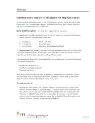
The exercises that follow compare the effect of the spectral resolution of different sensors on the
spectral signatures of minerals. The graph below shows the modeled effect of spectral resolution on the
appearance of spectral features for Kaolinite.
Spectral Modeling and Resolution
Spectral modeling shows that spectral resolution requirements for imaging spectrometers depend upon
the character of the material being measured. Kaolinite, for example (see the plot below), exhibits a
characteristic doublet near 2.2 µm at 20 nm resolution. Even at 40 nm resolution, the asymmetrical shape
of the band may be enough to identify the mineral, even though the spectral features have not been fully
resolved.
Page 5 of 24
© 2013 Exelis Visual Information Solutions, Inc. All Rights Reserved. This information is not subject to the controls
of the International Traffic in Arms Regulations (ITAR) or the Export Administration Regulations (EAR). However,
this information may be restricted from transfer to various embargoed countries under U.S. laws and regulations.

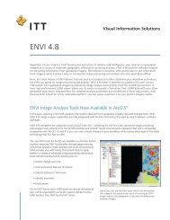
The spectral resolution required for a specific sensor is a direct function of the material you are trying to
identify, and the contrast between that material and the background materials. The following figure from
Swayze (1997) shows modeled spectra for kaolinite from several different sensors.
Page 6 of 24
© 2013 Exelis Visual Information Solutions, Inc. All Rights Reserved. This information is not subject to the controls
of the International Traffic in Arms Regulations (ITAR) or the Export Administration Regulations (EAR). However,
this information may be restricted from transfer to various embargoed countries under U.S. laws and regulations.

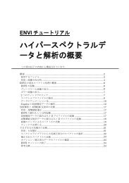
Case History: Cuprite, Nevada, USA
Cuprite has been used extensively as a test site for remote sensing instrument validation (Abrams et al.,
1978; Kahle and Goetz, 1983; Kruse et al., 1990; Hook et al., 1991). Refer to the following alteration
map of the region.
This tutorial illustrates the effects of spatial and spectral resolution on information extraction from
multispectral and hyperspectral data. You will use Landsat TM, GEOSCAN MkII, GER63, HyMap and
AVIRIS images of Cuprite, Nevada, USA, and you will see the effect of different spatial and spectral
resolutions on mineralogic mapping through remote sensing.
All of these datasets have been calibrated to reflectance. Only three of the numerous materials present
at the Cuprite site are used for comparison. Average kaolinite, alunite, and buddingtonite image spectra
were selected from known occurrences at Cuprite. Laboratory spectra from the USGS spectral library
(Clark et al., 1990) of the three selected minerals are provided for comparison to the image spectra.
Page 7 of 24
© 2013 Exelis Visual Information Solutions, Inc. All Rights Reserved. This information is not subject to the controls
of the International Traffic in Arms Regulations (ITAR) or the Export Administration Regulations (EAR). However,
this information may be restricted from transfer to various embargoed countries under U.S. laws and regulations.

Open and View USGS Library Spectra
1. From the ENVI® Classic main menu bar, select Spectral > Spectral Libraries > Spectral
Library Viewer. A Spectral Library Input File dialog appears.
2. Click Open and select Spectral Library. A file selection dialog appears.
3. Select usgs_em.sli. These spectra represent USGS laboratory measurements for kaolinite,
alunite, buddingtonite, and opal, in Cuprite, measured with a Beckman spectrometer. Click Open.
4. Select usgs_em.sli in the Spectral Library Input File dialog, and click OK. The Spectral
Library Viewer dialog appears.
5. In the Spectral Library Viewer dialog, select each mineral. The spectra appear in a Spectral
Library Plots window.
6. Examine the detail in the spectral plots, particularly the absorption feature positions, depths, and
shapes near 2.2 - 2.4 µm. For better comparison, use the middle mouse button to draw a box in the
plot window from 2.0 to 2.5 µm. Following is an annotated plot of laboratory spectra for kaolinite,
Page 8 of 24
© 2013 Exelis Visual Information Solutions, Inc. All Rights Reserved. This information is not subject to the controls
of the International Traffic in Arms Regulations (ITAR) or the Export Administration Regulations (EAR). However,
this information may be restricted from transfer to various embargoed countries under U.S. laws and regulations.

alunite, and buddingtonite, showing the absorption features of interest:
View Landsat TM Image and Spectra
The following plot shows region of interest (ROI) mean spectra for kaolinite, alunite, and buddingtonite.
The small squares indicate the TM band 7 (2.21 µm) center point. The lines indicate the slope from TM
band 5 (1.65 µm). The spectra appear very similar, and you cannot effectively discriminate between the
three endmembers.
Page 9 of 24
© 2013 Exelis Visual Information Solutions, Inc. All Rights Reserved. This information is not subject to the controls
of the International Traffic in Arms Regulations (ITAR) or the Export Administration Regulations (EAR). However,
this information may be restricted from transfer to various embargoed countries under U.S. laws and regulations.

View TM Mean Kaolinite and Alunite Image Spectra
1. From the ENVI Classic main menu bar, select Window > Start New Plot Window. A blank
ENVI Classic Plot Window appears.
2. From the ENVI Classic Plot Window menu bar, select File > Input Data > ASCII. A file
selection dialog appears.
3. Select cuptm_em.txt and click Open. An Input ASCII File dialog appears. Click OK to plot
the mean kaolinite and alunite spectra.
Compare Mean Spectra and Library Spectra
Refer to these steps throughout the rest of the tutorial whenever you compare library spectra and ROI
mean spectra from different sensors.
1. Right-click in the Spectral Library Plots window and select Plot Key.
2. Click and drag the Kaolinite and Alunite spectrum names from the Spectral Library Plots window
to the ENVI Classic Plot Window.
3. Right-click in the ENVI Classic Plot Window and select Plot Key.
Page 10 of 24
© 2013 Exelis Visual Information Solutions, Inc. All Rights Reserved. This information is not subject to the controls
of the International Traffic in Arms Regulations (ITAR) or the Export Administration Regulations (EAR). However,
this information may be restricted from transfer to various embargoed countries under U.S. laws and regulations.

4. For easier comparison, select Edit > Data Parameters from the ENVI Classic Plot Window
menu bar, and change the Mean:Kaolinite and Mean:Alunite colors to match the colors of the
corresponding library spectra.
Open Landsat TM Image
1. From the ENVI Classic main menu bar, select File > Open Image File. A file selection dialog
appears.
2. Select cuptm_rf.img. Click Open. This file contains Landsat TM data for Cuprite with a
spatial resolution of 30 m and a spectral resolution of up to 100 nm. These public-domain data
were acquired on 4 October 1984.
3. In the Available Bands List, select the Gray Scale radio button, select Band 6, and click Load
Band.
4. From the Display group menu bar, select Tools > Profiles > Z Profile (Spectrum). A Spectral
Profile plot window appears.
5. From the Display group menu bar, select Tools > Pixel Locator. A Pixel Locator dialog appears.
6. Enter the pixel location (248, 351), a kaolinite feature, and click Apply.
7. Right-click in the Spectral Profile plot window and select Collect Spectra.
8. Enter the following pixel locations and click Apply each time.
• Alunite (260, 330)
• Buddingtonite (202, 295)
• Silica or Opal (251, 297)
9. From the Spectral Profile menu bar, select Edit > Plot Parameters. A Plot Parameters dialog
appears.
10. The X-Axis radio button is selected by default. Enter Range values from 2.0 to 2.5. Click Apply,
then Cancel.
11. Right-click in the Spectral Profile window and select Stack Plots.
Page 11 of 24
© 2013 Exelis Visual Information Solutions, Inc. All Rights Reserved. This information is not subject to the controls
of the International Traffic in Arms Regulations (ITAR) or the Export Administration Regulations (EAR). However,
this information may be restricted from transfer to various embargoed countries under U.S. laws and regulations.

12. Compare the apparent reflectance spectra to the library spectra, by dragging and dropping spectra
from the ENVI Classic Plot Window into the Spectral Profile.
13. See "Draw Conclusions" on page 23, and answer some of the questions pertaining to Landsat TM
data.
14. When you are finished, close the display group, ENVI Classic Plot Window, and Spectral Profile.
Keep the Spectral Library Plots window open for the remaining exercises.
View GEOSCAN Image and Spectra
The GEOSCAN MkII sensor, flown on a light aircraft during the late 1980s, was a commercial aircraft
system that acquired up to 24 spectral channels selected from 46 available bands. GEOSCAN covered a
spectral range from 0.45 to 12.0 µm using grating dispersive optics and three sets of linear array
detectors (Lyon and Honey, 1989).
GEOSCAN's high spatial resolution makes it suitable for detailed geologic mapping (Hook et al., 1991).
A typical data acquisition for geology resulted in 10 bands in the visible/near infrared (VNIR, 0.52 - 0.96
µm), 8 bands in the shortwave infrared (SWIR, 2.04 - 2.35 µm), and thermal infrared (TIR, 8.64 - 11.28
µm) regions (Lyon and Honey, 1990). The relatively low number of spectral bands and low spectral
resolution limit mineralogic mapping to a few groups of minerals in the absence of ground information.
However, the strategic placement of the SWIR bands provides more mineralogic information than
expected under such limited spectral resolution.
The following plot shows ROI mean spectra for kaolinite, alunite, and buddingtonite. The spectra for
these minerals appear quite different in the GEOSCAN data, even with the relatively widely spaced
spectral bands.
Page 12 of 24
© 2013 Exelis Visual Information Solutions, Inc. All Rights Reserved. This information is not subject to the controls
of the International Traffic in Arms Regulations (ITAR) or the Export Administration Regulations (EAR). However,
this information may be restricted from transfer to various embargoed countries under U.S. laws and regulations.

View GEOSCAN Mean Kaolinite and Alunite Image Spectra
1. From the ENVI Classic main menu bar, select Window > Start New Plot Window. A blank
ENVI Classic Plot Window appears.
2. From the ENVI Classic Plot Window menu bar, select File > Input Data > ASCII. A file
selection dialog appears.
3. Select cupgs_em.txt and click Open. An Input ASCII File dialog appears. Click OK to plot
the kaolinite and alunite spectra in the ENVI Classic Plot Window.
4. Compare these spectra to the USGS library spectra (in the Spectral Library Plots window) and to
the spectra from the other sensors.
Open GEOSCAN Image
1. From the ENVI Classic main menu bar, select File > Open Image File. A file selection dialog
appears.
2. Select cupgs_sb.img. Click Open. This file contains GEOSCAN imagery of Cuprite
(collected in 1989), at approximately 60 nm spectral resolution with 44 nm sampling, converted to
apparent reflectance using a Flat Field correction in ENVI Classic.
3. To optionally view a color composite that enhances mineralogical differences, select the RGB
Color radio button, select Band 13, Band 15, and Band 18, and click Load RGB.
4. In the Available Bands List, select the Gray Scale radio button, select Band 15, and click Load
Band.
Page 13 of 24
© 2013 Exelis Visual Information Solutions, Inc. All Rights Reserved. This information is not subject to the controls
of the International Traffic in Arms Regulations (ITAR) or the Export Administration Regulations (EAR). However,
this information may be restricted from transfer to various embargoed countries under U.S. laws and regulations.

5. From the Display group menu bar, select Tools > Profiles > Z Profile (Spectrum). A Spectral
Profile plot window appears.
6. From the Display group menu bar, select Tools > Pixel Locator. A Pixel Locator dialog appears.
7. Enter the pixel location (275, 761), a kaolinite feature, and click Apply.
8. Right-click in the Spectral Profile plot window and select Collect Spectra.
9. Enter the following pixel locations and click Apply each time.
Alunite (435, 551)
Buddingtonite (168, 475)
Silica or Opal (371, 592)
10. From the Spectral Profile menu bar, select Edit > Plot Parameters. A Plot Parameters dialog
appears.
11. The X-Axis radio button is selected by default. Enter Range values from 2.0 to 2.5. Click Apply,
then Cancel.
12. Right-click in the Spectral Profile window and select Stack Plots.
13. Compare the GEOSCAN image spectra to the library spectra (in the Spectral Library Plots
window) and to the Landsat TM spectra.
14. See "Draw Conclusions" on page 23, and answer some of the questions pertaining to GEOSCAN
data.
15. When you are finished, close the display group, ENVI Classic Plot Window, and Spectral Profile.
Keep the Spectral Library Plots window open for the remaining exercises.
Page 14 of 24
© 2013 Exelis Visual Information Solutions, Inc. All Rights Reserved. This information is not subject to the controls
of the International Traffic in Arms Regulations (ITAR) or the Export Administration Regulations (EAR). However,
this information may be restricted from transfer to various embargoed countries under U.S. laws and regulations.

View GER63 Image and Spectra
The Geophysical and Environmental Research 63-band scanner (GER63) has an advertised spectral
resolution of 17.5 nm, but comparison with other sensors and laboratory spectra suggests that 35 nm
resolution with 17.5 nm sampling is more likely. Four bad bands were dropped so that only 59 spectral
bands are available. The GER63 data used in this exercise were acquired during August 1987. Selected
analysis results were previously published in Kruse et al. (1990).
The plot below shows the ROI mean spectra for kaolinite, alunite, and buddingtonite. The GER63 data
adequately discriminate alunite and buddingtonite, but they do not fully resolve the kaolinite “doublet”
near 2.2 µm shown in the laboratory spectra.
View GER63 Mean Kaolinite and Alunite Image Spectra
1. From the ENVI Classic main menu bar, select Window > Start New Plot Window. A blank
ENVI Classic Plot Window appears.
2. From the ENVI Classic Plot Window menu bar, select File > Input Data > ASCII. A file
selection dialog appears.
Page 15 of 24
© 2013 Exelis Visual Information Solutions, Inc. All Rights Reserved. This information is not subject to the controls
of the International Traffic in Arms Regulations (ITAR) or the Export Administration Regulations (EAR). However,
this information may be restricted from transfer to various embargoed countries under U.S. laws and regulations.

3. Select cupgerem.txt and click Open. An Input ASCII File dialog appears. Click OK to plot
the kaolinite and alunite spectra in the ENVI Classic Plot Window.
4. Compare these spectra to the USGS library spectra (in the Spectral Library Plots window) and to
the spectra from the other sensors.
Open GER63 Image
1. From the ENVI Classic main menu bar, select File > Open Image File. A file selection dialog
appears.
2. Select cupgersb.img. Click Open.
3. To optionally view a color composite that enhances mineralogical differences, select the RGB
Color radio button, select Band 36, Band 42, and Band 50, and click Load RGB.
4. In the Available Bands List, select the Gray Scale radio button, select Band 42, and click Load
Band.
5. From the Display group menu bar, select Tools > Profiles > Z Profile (Spectrum). A Spectral
Profile plot window appears.
6. From the Display group menu bar, select Tools > Pixel Locator. A Pixel Locator dialog appears.
7. Enter the pixel location (235, 322), a kaolinite feature, and click Apply.
8. Right-click in the Spectral Profile plot window and select Collect Spectra.
9. Enter the following pixel locations and click Apply each time.
• Alunite (303, 240)
• Buddingtonite (185, 233)
• Silica or Opal (289, 253)
10. From the Spectral Profile menu bar, select Edit > Plot Parameters. A Plot Parameters dialog
appears.
11. The X-Axis radio button is selected by default. Enter Range values from 2.0 to 2.5. Click Apply,
then Cancel.
12. Right-click in the Spectral Profile window and select Stack Plots.
Page 16 of 24
© 2013 Exelis Visual Information Solutions, Inc. All Rights Reserved. This information is not subject to the controls
of the International Traffic in Arms Regulations (ITAR) or the Export Administration Regulations (EAR). However,
this information may be restricted from transfer to various embargoed countries under U.S. laws and regulations.

13. Compare the GER63 image spectra to the library spectra (in the Spectral Library Plots window)
and to spectra from the other sensors.
14. See"Draw Conclusions" on page 23, and answer some of the questions pertaining to GER63 data.
15. When you are finished, close the display group, ENVI Classic Plot Window, and Spectral Profile.
Keep the Spectral Library Plots window open for the remaining exercises.
View HyMap Image and Spectra
HyMap is a state-of-the-art, aircraft-mounted, hyperspectral sensor developed by Integrated Spectronics,
Sydney, Australia, and operated by HyVista Corporation. HyMap provides unprecedented spatial,
spectral and radiometric resolution (Cocks et al., 1998). The system has a whiskbroom scanner utilizing
diffraction gratings and four 32-element detector arrays to provide 126 spectral channels covering the
0.44 - 2.5 µm range over a 512-pixel swath. Spectral resolution varies from 10 - 20 nm with 3 – 10 m
spatial resolution and a signal-to-noise ratio over 1000:1. The HyMap data described here were acquired
on September 11, 1999. Selected analysis results were published in Kruse et al. (1999). The plot below
shows ROI mean spectra for kaolinite, alunite, and buddingtonite.
Page 17 of 24
© 2013 Exelis Visual Information Solutions, Inc. All Rights Reserved. This information is not subject to the controls
of the International Traffic in Arms Regulations (ITAR) or the Export Administration Regulations (EAR). However,
this information may be restricted from transfer to various embargoed countries under U.S. laws and regulations.

View HyMap Mean Kaolinite and Alunite Image Spectra
1. From the ENVI Classic main menu bar, select Window > Start New Plot Window. A blank
ENVI Classic Plot Window appears.
2. From the ENVI Classic Plot Window menu bar, select File > Input Data > ASCII. A file
selection dialog appears.
3. Select cup99hy_em.txt. Click Open. An Input ASCII File dialog appears. Click OK to plot
the kaolinite and alunite spectra in the ENVI Classic Plot Window.
4. Compare these spectra to the USGS library spectra (in the Spectral Library Plots window) and to
the spectra from the other sensors.
Open HyMap Image
1. From the ENVI Classic main menu bar, select File > Open Image File. A file selection dialog
appears.
Page 18 of 24
© 2013 Exelis Visual Information Solutions, Inc. All Rights Reserved. This information is not subject to the controls
of the International Traffic in Arms Regulations (ITAR) or the Export Administration Regulations (EAR). However,
this information may be restricted from transfer to various embargoed countries under U.S. laws and regulations.

2. Select cup99hy.eff. Click Open. This file contains HyMap EFFORT-polished,
atmospherically corrected apparent reflectance data. The data are rotated 180 degrees from north,
so north is at the bottom of the image.
3. To optionally view a color composite that enhances mineralogical differences, select the RGB
Color radio button, select Band 104, Band 109, and Band 117, and click Load RGB.
4. In the Available Bands List, select the Gray Scale radio button, select Band 109, and click Load
Band.
5. From the Display group menu bar, select Tools > Profiles > Z Profile (Spectrum). A Spectral
Profile plot window appears.
6. From the Display group menu bar, select Tools > Pixel Locator. A Pixel Locator dialog appears.
7. Enter the pixel location (248, 401), a kaolinite feature, and click Apply.
8. Right-click in the Spectral Profile plot window and select Collect Spectra.
9. Enter the following pixel locations and click Apply each time.
• Alunite: (184, 568)
• Buddingtonite: (370, 594)
• Silica or Opal: (172, 629)
10. From the Spectral Profile menu bar, select Edit > Plot Parameters. A Plot Parameters dialog
appears.
11. The X-Axis radio button is selected by default. Enter Range values from 2.0 to 2.5. Click Apply,
then Cancel.
12. Right-click in the Spectral Profile window and select Stack Plots.
13. Compare the HyMap image spectra to the library spectra (in the Spectral Library Plots window)
and to spectra from the other sensors.
14. See "Draw Conclusions" on page 23, and answer some of the questions pertaining to HyMap data.
15. When you are finished, close the display group, ENVI Classic Plot Window, and Spectral Profile.
Keep the Spectral Library Plots window open for the remaining exercise.
Page 19 of 24
© 2013 Exelis Visual Information Solutions, Inc. All Rights Reserved. This information is not subject to the controls
of the International Traffic in Arms Regulations (ITAR) or the Export Administration Regulations (EAR). However,
this information may be restricted from transfer to various embargoed countries under U.S. laws and regulations.

View AVIRIS Image and Spectra
AVIRIS data have approximately 10 nm spectral resolution and 20 m spatial resolution. The AVIRIS
data used in this exercise were acquired during July 1995 as part of an AVIRIS Group Shoot (Kruse and
Huntington, 1996). The following plot shows the ROI mean spectra for kaolinite, alunite, and
buddingtonite. Compare these to the library spectra and note the high quality and nearly identical
signatures.
Page 20 of 24
© 2013 Exelis Visual Information Solutions, Inc. All Rights Reserved. This information is not subject to the controls
of the International Traffic in Arms Regulations (ITAR) or the Export Administration Regulations (EAR). However,
this information may be restricted from transfer to various embargoed countries under U.S. laws and regulations.

View AVIRIS Mean Kaolinite and Alunite Image Spectra
1. From the ENVI Classic main menu bar, select Window > Start New Plot Window. A blank
ENVI Classic Plot Window appears.
2. From the ENVI Classic Plot Window menu bar, select File > Input Data > ASCII. A file
selection dialog appears.
3. Select cup95eff.txt. Click Open. An Input ASCII File dialog appears. Click OK to plot the
kaolinite and alunite spectra in the ENVI Classic Plot Window.
4. Compare these spectra to the USGS library spectra (in the Spectral Library Plots window) and to
the spectra from the other sensors.
Open AVIRIS Image
1. From the ENVI Classic main menu bar, select File > Open Image File. A file selection dialog
appears.
2. Select cup95eff.int. Click Open. A color composite of bands 183, 193, and 207
automatically loads in a new display group.
3. In the Available Bands List, select the Gray Scale radio button, select Band 193, and click Load
Band.
4. From the Display group menu bar, select Tools > Profiles > Z Profile (Spectrum). A Spectral
Profile plot window appears.
Page 21 of 24
© 2013 Exelis Visual Information Solutions, Inc. All Rights Reserved. This information is not subject to the controls
of the International Traffic in Arms Regulations (ITAR) or the Export Administration Regulations (EAR). However,
this information may be restricted from transfer to various embargoed countries under U.S. laws and regulations.

5. From the Display group menu bar, select Tools > Pixel Locator. A Pixel Locator dialog appears.
6. Enter the pixel location (500, 581), which is a Kaolinite feature, and click Apply.
7. Right-click in the Spectral Profile plot window and select Collect Spectra.
8. Enter the following pixel locations and click Apply each time.
• Alunite (538, 536)
• Buddingtonite (447, 484)
• Silica or Opal (525, 505)
9. From the Spectral Profile menu bar, select Edit > Plot Parameters. A Plot Parameters dialog
appears.
10. The X-Axis radio button is selected by default. Enter Range values from 2.0 to 2.5. Click Apply,
then Cancel.
11. Right-click in the Spectral Profile window and select Stack Plots.
12. Compare the AVIRIS image spectra to the library spectra (in the Spectral Library Plots window)
and to spectra from the other sensors.
13. See"Draw Conclusions" on page 23, and answer some of the questions pertaining to AVIRIS
data.
Page 22 of 24
© 2013 Exelis Visual Information Solutions, Inc. All Rights Reserved. This information is not subject to the controls
of the International Traffic in Arms Regulations (ITAR) or the Export Administration Regulations (EAR). However,
this information may be restricted from transfer to various embargoed countries under U.S. laws and regulations.

Draw Conclusions
The four sensors and the library spectra that you have evaluated represent a broad range of spectral
resolutions. Using the USGS library spectra as ground truth, evaluate how well each of the sensors
represents the ground truth information. Consider what it means to discriminate between materials
versus identification of materials.
Consider the following questions:
1. From the library spectra, what is the minimum spacing of absorption features in the 2.0 - 2.5 µm
range
2. The TM data dramatically undersample the 2.0 - 2.5 µm range, as only TM band 7 is available.
What evidence do you see for absorption features in this range What differences are apparent in
the TM spectra of minerals with absorption features in this range
3. The GEOSCAN data also undersample the 2.0 - 2.5 µm range, however, the bands are
strategically placed. What differences do you see between the GEOSCAN spectra for the
different minerals Could some of the bands have been placed differently to provide better
mapping of specific minerals
4. The GER63 data provide improved spectral resolution over the GEOSCAN data, and you can
observe individual features. The advertised spectral resolution of the GER63 between 2.0 - 2.5
µm is 17.5 nm. Examine the GER63 kaolinite spectrum and defend or refute this specification. Do
the more closely spaced spectral bands of the GER63 sensor provide a significant advantage over
the GEOSCAN data in mapping and identifying these reference minerals
5. What are the main differences between mineral spectra at Cuprite caused by the change from 10
nm spectral resolution (AVIRIS) to 17 nm spectral resolution (HyMap)
6. The AVIRIS data provide the best spectral resolution of the sensors examined here. How do the
AVIRIS and laboratory spectra compare What are the major similarities and differences What
factors affect the comparison of the two data types
7. Examine all of the images and spectra. What role does spatial resolution play in the comparison
8. Based on the library spectra, provide sensor spectral and spatial resolution design specifications
as well as recommendations on placement of spectral bands for mineral mapping. Examine the
trade-offs between continuous high-spectral resolution bands and strategically placed, lowerresolution
bands.
Copyright Notice:
ENVI Classic is a registered trademark of Exelis Inc.
QUAC and FLAASH are registered trademarks of Spectral Sciences, Inc.
Page 23 of 24
© 2013 Exelis Visual Information Solutions, Inc. All Rights Reserved. This information is not subject to the controls
of the International Traffic in Arms Regulations (ITAR) or the Export Administration Regulations (EAR). However,
this information may be restricted from transfer to various embargoed countries under U.S. laws and regulations.