Homework Problem Set 5 Solutions ( )2

Chemistry 380.37
Dr. Jean M. Standard
Homework Problem Set 5 Solutions
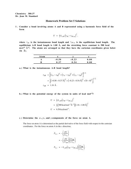
1. Consider a bond involving atoms A and B represented using a harmonic force field of the
form
U = 1 2 k s,AB
( r AB − r AB,eq ) 2 ,
where r AB is the instantaneous bond length and r AB,eq is the equilibrium bond length. The
equilibrium A-B bond length € is 1.00 Å, and the stretching force constant is 500 kcal
mol –1 Å –2 . The atoms are arranged so that they have the cartesian coordinates given below
€ (in Å).
€
Atom x y z
A –0.50 –0.23 0.00
B 0.37 0.54 0.00
a.) What is the instantaneous A-B bond length
[( ) 2 + ( y A − y ) 2 B + ( z A − z ) 2
] 1/ 2
B
r AB = x A − x B
( ) 2 + ( −0.23 − 0.54 Å) 2 + 0 − 0
= ⎡⎡ −0.50 − 0.37 Å
⎣⎣ ⎢⎢
r AB = 1.16 Å .
( ) 2
1/ 2
⎤⎤
⎦⎦ ⎥⎥
b.) What is the € potential energy of the system in units of kcal mol –1
U = 1 2 k s,AB ( r AB − r AB,eq ) 2
= 1 2 ( 500 kcalmol−1 Å −2
)( 1.16−1.00 Å) 2
U = 6.56 kcalmol −1 .
c.) Determine the x-, € y-, and z-components of the force on atom A.
The force on atom A is determined as the partial derivative of the force field with respect to the cartesian
coordinates. For the force on atom A in the x direction,
⎛⎛
F A,x = −
∂U ⎞⎞
⎜⎜ ⎟⎟
⎝⎝ ∂ x A ⎠⎠
⎛⎛
= − ∂U ⎞⎞ ⎛⎛
⎜⎜ ⎟⎟ ∂ r ⎞⎞
AB
⎜⎜ ⎟⎟
⎝⎝ ∂ r AB ⎠⎠ ⎝⎝ ∂ x A ⎠⎠
⎛⎛
F A,x = − k s,AB ( r AB − r AB,eq ) ∂ r ⎞⎞
AB
⎜⎜ ⎟⎟ .
⎝⎝ ∂ x A ⎠⎠
€

1 c.) continued
2
To complete the derivation of the force, the derivative of the bond length
coordinate x A must be determined.
r AB with respect to the cartesian
⎛⎛ ∂ r AB ⎞⎞
⎜⎜ ⎟⎟ = 1 x
⎝⎝ ∂ x A ⎠⎠ 2 [ ( A − x ) 2 B + ( y A − y ) 2 B + ( z A − z ) 2
] −1/ 2 B 2
⎛⎛ ∂ r AB ⎞⎞
⎜⎜ ⎟⎟ = x A − x B
.
⎝⎝ ∂ x A ⎠⎠ r AB
( )
( ) x A − x B
Substituting,
€
⎛⎛
F A,x = − k s,AB ( r AB − r AB,eq ) x A − x ⎞⎞
B
⎜⎜ ⎟⎟
⎝⎝ ⎠⎠
r AB
= − ( 500 kcalmol −1 Å −2
)( 1.16−1.00 Å) F A,x = 60.6 kcalmol −1 Å −1 .
⎛⎛
⎜⎜
⎝⎝
−0.50− 0.37 Å
1.16 Å
⎞⎞
⎟⎟
⎠⎠
€
Similarly, the y-component of the force can be calculated,
€
⎛⎛
F A,y = − k s,AB ( r AB − r AB,eq ) y A − y ⎞⎞
B
⎜⎜ ⎟⎟
⎝⎝ ⎠⎠
r AB
= − ( 500 kcalmol −1 Å −2
)( 1.16−1.00 Å) F A,y = 53.6 kcalmol −1 Å −1 .
⎛⎛
⎜⎜
⎝⎝
−0.23− 0.54 Å
1.16 Å
⎞⎞
⎟⎟
⎠⎠
Finally, the z-component is calculated,
€
⎛⎛
F A,z = − k s,AB ( r AB − r AB,eq ) z A − z ⎞⎞
B
⎜⎜ ⎟⎟
⎝⎝ ⎠⎠
r AB
= − ( 500 kcalmol −1 Å −2
)( 1.16−1.00 Å) F A,z = 0.
⎛⎛
⎜⎜
⎝⎝
0.0− 0.0 Å
1.16 Å
⎞⎞
⎟⎟
⎠⎠
d.) Determine the € x-, y-, and z-components of the force on atom B.
The force on atom B is determined as the partial derivative of the force field with respect to the cartesian
coordinates. As in part (c) above, the x component of the force on atom B is
⎛⎛
F B,x = −
∂U ⎞⎞
⎜⎜ ⎟⎟
⎝⎝ ∂ x B ⎠⎠
⎛⎛
= − ∂U ⎞⎞ ⎛⎛
⎜⎜ ⎟⎟ ∂ r ⎞⎞
AB
⎜⎜ ⎟⎟
⎝⎝ ∂ r AB ⎠⎠ ⎝⎝ ∂ x B ⎠⎠
⎛⎛
F B,x = − k s,AB ( r AB − r AB,eq ) ∂ r ⎞⎞
AB
⎜⎜ ⎟⎟ .
⎝⎝ ∂ x B ⎠⎠
€

1 d.) continued
3
To complete the derivation of the force, the derivative of the bond length
coordinate x B must be determined.
r AB with respect to the cartesian
⎛⎛ ∂ r AB ⎞⎞
⎜⎜ ⎟⎟ = 1 x
⎝⎝ ∂ x B ⎠⎠ 2 [ ( A − x ) 2 B + ( y A − y ) 2 B + ( z A − z ) 2
] −1/ 2 B −2
⎛⎛ ∂ r AB ⎞⎞
⎜⎜ ⎟⎟ = − x A − x B
.
⎝⎝ ∂ x B ⎠⎠ r AB
( )
( ) x A − x B
Substituting,
€
⎛⎛
F B,x = k s,AB ( r AB − r AB,eq ) x A − x ⎞⎞
B
⎜⎜ ⎟⎟
⎝⎝ ⎠⎠
r AB
= ( 500 kcalmol −1 Å −2
)( 1.16−1.00 Å) F B,x = − 60.6 kcalmol −1 Å −1 .
⎛⎛
⎜⎜
⎝⎝
−0.50− 0.37 Å
1.16 Å
⎞⎞
⎟⎟
⎠⎠
€
Similarly, the y-component of the force can be calculated,
€
⎛⎛
F B,y = k s,AB ( r AB − r AB,eq ) y A − y ⎞⎞
B
⎜⎜ ⎟⎟
⎝⎝ ⎠⎠
r AB
= ( 500 kcalmol −1 Å −2
)( 1.16−1.00 Å) F B,y = − 53.6 kcalmol −1 Å −1 .
⎛⎛
⎜⎜
⎝⎝
−0.23− 0.54 Å
1.16 Å
⎞⎞
⎟⎟
⎠⎠
Finally, the z-component is calculated,
€
⎛⎛
F B,z = k s,AB ( r AB − r AB,eq ) z A − z ⎞⎞
B
⎜⎜ ⎟⎟
⎝⎝ ⎠⎠
r AB
= ( 500 kcalmol −1 Å −2
)( 1.16−1.00 Å) F B,z = 0.
⎛⎛
⎜⎜
⎝⎝
0.0− 0.0 Å
1.16 Å
⎞⎞
⎟⎟
⎠⎠
€

4
1. continued
e.) Are the atoms moving closer together or farther apart
The positions of the two atoms are shown in the figure below (note that the force vectors are not drawn to
scale). The force on atom A is in the positive x and positive y direction (along the bond). The force on
atom B is in the negative x and negative y direction (also along the bond). Thus, the atoms are moving
closer together.
1.0
0.5
B
y (Å)
0.0
-0.5
A
-1.0
-1.0 -0.5 0.0 0.5 1.0
x (Å)
2. Consider the simple one-dimensional harmonic potential as a representation of the motion
of a bond in a molecular system,
U( x) = 1 2 k x 2 .
The coordinate x represents the bond displacement, x = r − r eq. Assume that the force
constant k for the bond is 720 € kcal mol –1 Å –2 . The reduced mass is 12.0 g/mol. The
bond displacement coordinate has an initial value of 0 Å. The initial velocity is 8400
m/s.
€
a.) What is the potential energy
U = 1 2 kx 2
= 1 2 720 kcalmol−1 Å −2
U = 0.
( ) 0
( ) 2
€

2. continued
5
b.) What is the kinetic energy of the system
T = 1 2 mv 2
= 1 2
( 0.012 kg mol−1) 8400 ms −1
( ) 2
= 4.23×10 5 J/mol
T = 1.01×10 5 cal/mol (or 101 kcal/mol).
c.) What is the total € energy of the system
E = T + U
= 101 + 0 kcal/mol
E = 101 kcal/mol.
€

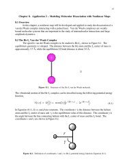
3. Consider the potential energy function studied in problem 2 with the same parameters.
Since the potential energy function described in problem 2 is harmonic, the bond
undergoes simple harmonic motion as a function of time. The exact analytical solutions
of Newton's equations for a harmonic oscillator with an initial position of zero and an
initial velocity v(0) are
6
€
x(t) = v(0)
ω
sin( ω t)
v(t) = v(0) cos( ω t) .
The parameter ω is the angular velocity and is defined by the relation
ω =
where m is the mass. The angular velocity ω is related to the harmonic frequency of
oscillation ν o ,
€
k
m ,
€
ν o =
ω
2π .
a.) Using the same parameters as € given in problem 2, determine the harmonic frequency of
vibration for this system.
For simple harmonic motion, the harmonic frequency of vibration ν o is
ν o =
=
ω
2π = 1
2π
1
2π
ν o = 2.52 ×10 13 s −1 .
k
m
€
⎛⎛ 720 kcalmol −1 Å −2 ⎞⎞ ⎛⎛ 4.184 kJ
⎜⎜
⎝⎝ 0.012 kg mol −1 ⎟⎟ ⎜⎜
⎠⎠ ⎝⎝ 1kcal
⎞⎞ ⎛⎛
⎟⎟ 1000 J ⎞⎞ ⎛⎛ 1Å ⎞⎞
⎜⎜ ⎟⎟ ⎜⎜
⎠⎠ ⎝⎝ 1kJ ⎠⎠ ⎝⎝ 10 −10 ⎟⎟
m⎠⎠
2
€

3. continued
7
b.) Using the analytic solution to Newton's equations for the harmonic oscillator, plot the
bond displacement coordinate x as a function of time.
For simple harmonic motion and the provided initial conditions, the analytic expression for the position is
x(t) = v(0)
ω
sin( ω t)
.
Using the harmonic vibrational frequency ν o calculated in part (a), the angular frequency ω can be
determined,
€
€
ω = 2π ν o
( )
= 2π 2.52 ×10 13 s −1
ω = 1.58 ×10 14 s −1 .
The initial velocity is
€
v( 0) = 8400 m/s . Thus, the position as a function of time is given by the equation
€
( ) = v(0)
x t
sin( ω t)
ω
⎛⎛ 8400 m/s ⎞⎞
= ⎜⎜
⎝⎝ 1.58 ×10 14 s −1 ⎟⎟ sin 1.58 ×10 14 s −1 t
⎠⎠
= 5.31×10 −11 m
( )
( ) sin( 1.58 ×10 14 s −1 t)
( ) sin( 1.58 ×10 14 s −1 t) .
x( t) = 0.531Å
A plot of this function versus time is shown in the figure below.
0.6
€
0.4
0.2
x(t) (Å)
0.0
0.0 0.1 0.2 0.3 0.4 0.5
-0.2
-0.4
-0.6
time (ps)

3. continued
8
c.) Using the analytic solution to Newton's equations for the harmonic oscillator, plot the
velocity as a function of time.
The velocity is the time derivative of the position,
€
( ) = x ˙ ( t) = d dt x( t)
v t
= d dt
⎡⎡ v(0)
⎣⎣
⎢⎢
ω
sin( ω t)
⎤⎤
⎦⎦
⎥⎥
v( t) = v( 0) cos( ω t ) .
Substituting the specific parameters for this problem, the expression for the velocity becomes
v( t) = ( 8400 m/s) cos( 1.58 ×10 14 s −1 t),
with the velocity in m/s and the frequency in s –1 . A plot of the velocity as a function of time is shown in
the figure below. €
10000
8000
6000
4000
v(t) (m/s)
2000
0
0.0 0.1 0.2 0.3 0.4 0.5
-2000
-4000
-6000
-8000
-10000
time (ps)

4. Again consider the simple one-dimensional potential used in problems 2 and 3. Assume
that the force constant k is 720 kcal mol –1 Å –2 . The reduced mass is 12.0 g/mol. The
initial position is 0 Å and the initial velocity is 8400 m/s.
9
a.) Using the Verlet leapfrog algorithm, carry out two time steps to determine the
position and velocity of the particle at times t 1 and t 2 . Use a step size of 1
femtosecond.
The Verlet leapfrog algorithm for one particle in one dimension is given by
x( t n+1 ) = x( t n ) + hv x ( t n+1/ 2 )
v x ( t n+1/ 2 ) = v x ( t n−1/ 2 ) + h m F x( t n) .
The force F x is obtained from the force field,
€
F x = − dU
dx
F x = − kx .
Subsituting, the velocity equation becomes
€
( ) = v x ( t n−1/ 2 ) − hk m x t n
v x t n+1/ 2
( ).
For n = 0, the Verlet leapfrog equations are given by
v x ( t 1/ 2 ) = v x ( t −1/ 2 ) − hk
m x t 0
x( t 1 ) = x( t 0 ) + h v x ( t 1/ 2 ) .
The time step is h = 10 −15 s . Using the initial conditions x t 0
v x ( t −1/2 ) = v x ( 0) = 8400 € m/s, the velocity equations is
The position equation then becomes
€
( )
v x ( t 1/ 2 ) = v x ( t −1/ 2 ) − hk
m x ( t 0)
= 8400 m/s − hk
m ( 0)
v x ( t 1/ 2 ) = 8400 m/s.
x( t 1 ) = x( t 0 ) + h v x ( t 1/ 2 )
= 0 + ( 10 −15 s) ( 8400 m/s)
x( t 1 ) = 8.40 × 10 −12 m.
( ) = x( 0) = 0 and
€

4 a.) continued
10
For the next time step, with n = 1, the velocity equation becomes
v x ( t 3/ 2 ) = v x ( t 1/2 ) − hk
m x ( t 1).
In order to evaluate this equation, it is helpful to convert the force constant into SI units,
€
v x t 3/ 2
k = ( 760 kcalmol −1 Å −2 ⎛⎛ 4.184 kJ ⎞⎞
) ⎜⎜ ⎟⎟ 1000 J
2
⎛⎛ ⎞⎞ ⎛⎛
1Å
⎞⎞
⎜⎜ ⎟⎟ ⎜⎜
⎝⎝ 1kcal ⎠⎠ ⎝⎝ 1kJ ⎜⎜
⎠⎠ ⎝⎝ 10 −10 ⎟⎟
⎟⎟
m⎠⎠
k = 3.01×10 26 J mol −1 m −2 .
Substituting the force constant into the velocity equation yields
€
( ) = v x ( t 1/ 2 ) − hk
( )
m x t 1
= 8400 m/s − 10−15 s
v x ( t 3/ 2 ) = 8189 m/s.
For the time step with n = 1 the position equation becomes
( )( 3.01× 10 26 J mol −1 m −2 )( 8.40 × 10 −12 m)
( 0.012 kg mol −1 )
x( t 2 ) = x( t 1 ) + h v x ( t 3/ 2 ) .
Substituting,
€
x t 2
( )
( ) = 8.40 ×10 −12 m + 10 −15 s ( 8189 m/s )
x( t 2 ) = 1.66 ×10 −11 m.
Finally, for the final time step, with n = 2, the velocity equation becomes
€
€
v x ( t 5/ 2 ) = v x ( t 3/ 2 ) − hk
m x ( t 2).
Using the force constant in the velocity equation yields
€
v x ( t 5/ 2 ) = 8189 m/s −
v x ( t 5/ 2 ) = 7773 m/s.
Averaging the first pair of velocities, the equations are
v x t 0
( 10 −15 s) 3.01×1026 J mol −1 m −2
( )( 1.66 ×10−11 m)
( 0.012 kg mol −1
)
( ) = 1 2
[ v x( t 1/ 2) + v x ( t −1/ 2 )]
= 1 [ 8400 m/s + 8400 m/s ]
2
v x ( t 0 ) = 8400 m/s.
€

4 a.) continued
11
Averaging the second pair of velocities yields
€
( ) = 1 2 [ v x( t 3/ 2) + v x ( t 1/ 2 )]
= 1 [ 8189 m/s + 8400 m/s ]
2
( ) = 8295m/s.
v x t 1
v x t 1
Averaging the final pair of velocities yields
€
( ) = 1 2 [ v x( t 5/ 2) + v x ( t 3/ 2 )]
= 1 [ 7773m/s + 8189 m/s ]
2
( ) = 7981m/s.
v x t 2
v x t 2
These results are summarized in the table below.
n
t n
(s)
x( t n )
(m)
v x ( t n )
(m/s)
0 0 0 8400
1 1×10 −15 8.40× 10 −12 8295
2 2× 10 −15 1.66 ×10 −11 7981
b.) Compare your results from part (a) to the exact solution obtained in problem 3.
The equations for the exact analytic solutions for the position and velocity are given in problem 3. The
position is
€
x( t) = ( 0.531 Å)sin( 1.58 ×10 14 s −1 t) ,
with time in seconds and position in angstroms. The velocity is
v( t) = ( 8400 m/s) cos( 1.58 ×10 14 s −1 t) ,
€
€
with the velocity in m/s and time in seconds. The results for the analytic solution, using the same time
points as in part (b), yields € the results presented in the table below.
n
t n
(s)
x( t n )
(m)
v x ( t n )
(m/s)
0 0 0 8400
1 1×10 −15 8.363×10 −12 8295
2 2× 10 −15 1.652 ×10 −11 7982
We can see from these results that the leapfrog algorithm predicts the velocities with little error compared to
the analytic solution. The percent errors for the n = 0, 1, and 2 time steps are 0%, 0%, and 0.01%,
respectively. The leapfrog algorithm also does a reasonable job in predicting the position of the particle
compared to the analytic solution. The errors are somewhat larger than those for the velocity, with errors of
0%, 0.4%, and 0.6%, respectively.

5. The Maxwell-Boltzmann distribution for speeds is
12
F(v) = 4π v 2
3/ 2
⎛⎛ m ⎞⎞
⎜⎜ ⎟⎟
⎝⎝ 2π k B T ⎠⎠
⎛⎛
exp − mv2 ⎞⎞
⎜⎜
⎝⎝ 2k B T
⎟⎟ .
⎠⎠
In this equation, m is the mass of a particle, k B is the Boltzmann constant, T is
temperature, and v € is the speed.
velocity vector,
where
v x ,
v y, and
The most probable speed
€ by € the equation €
The speed v is defined to be the magnitude of the
2
v = v x +
2 vy +
2
[ vz ] 1/ 2 ,
v z are the components of the velocity vector.
€
v mp corresponding to the maximum in the distribution is given
€
v mp =
⎛⎛
⎜⎜
⎝⎝
2k B T
m
1/ 2
⎞⎞
⎟⎟ .
⎠⎠
a.) Plot the Maxwell-Boltzmann distribution function F(v) (y-axis) versus v (x-axis) for a
collection of atoms at 300 € K. Assume that one mole of atoms weighs 12.0 g.
b.)
Using the same mass as in part (a), plot € the Maxwell-Boltzmann distribution function
F(v) versus v for a collection of atoms at 1000 K. Discuss the effect of temperature
on the distribution of atomic speeds.
€
Both questions (a) and (b) are answered below.
The Maxwell-Boltzmann distribution function for the atoms at 300 K is given by
⎢⎢ 0.012 kg/mol
( ) = 4π v 2 ⎢⎢
F v
3/ 2
⎡⎡
⎛⎛ 1mol ⎞⎞ ⎤⎤
( ) ⎜⎜
⎝⎝ 6.02217 × 10 23 ⎟⎟
⎠⎠
⎥⎥
⎥⎥
⎢⎢ 2π( 1.38062 × 10 -23 JK −1 )( 300 K)
⎥⎥
⎢⎢
⎥⎥
⎣⎣
⎦⎦
⎧⎧
⎛⎛ 1mol ⎞⎞
( 0.012 kg/mol)
⎜⎜
⎝⎝ 6.02217 × 10
× exp −
23 ⎟⎟ v 2 ⎫⎫
⎪⎪
⎠⎠
⎪⎪
⎪⎪
⎪⎪
⎨⎨
2( 1.38062 × 10 -23 JK −1 ⎬⎬
⎪⎪
)( 300 K)
⎪⎪
⎩⎩ ⎪⎪
⎭⎭ ⎪⎪
€
F( v) = ( 8.41956 × 10 −9 v 2 ) exp{ −2.40549 × 10 −6 v 2 }.
€

5a, b.) continued
13
The velocity distribution function for the atoms at 1000 K is given by
€
⎢⎢ 0.012 kg/mol
( ) = 4π v 2 ⎢⎢
F v
3/ 2
⎡⎡
⎛⎛ 1mol ⎞⎞ ⎤⎤
( ) ⎜⎜
⎝⎝ 6.02217 × 10 23 ⎟⎟
⎠⎠
⎥⎥
⎥⎥
⎢⎢ 2π( 1.38062 × 10 -23 JK −1 )( 1000 K)
⎥⎥
⎢⎢
⎥⎥
⎣⎣
⎦⎦
⎧⎧
⎛⎛ 1mol ⎞⎞
( 0.012 kg/mol)
⎜⎜
⎝⎝ 6.02217 × 10
× exp −
23 ⎟⎟ v 2 ⎫⎫
⎪⎪
⎠⎠
⎪⎪
⎪⎪
⎪⎪
⎨⎨
2( 1.38062 × 10 -23 JK −1 ⎬⎬
⎪⎪
)( 1000 K)
⎪⎪
⎩⎩ ⎪⎪
⎭⎭ ⎪⎪
F( v) = ( 1.38347 × 10 −9 v 2 ) exp{ −7.21646 × 10 −7 v 2 }.
Note that the units of the exponent cancel out so that it is unitless, while the units of the terms in front of
the exponent are € sm –1 .
Plots of the Maxwell-Boltzmann distribution of speeds at 300 and 1000 K are shown on a single graph
below.
0.0014
0.0012
T = 300 K
0.0010
F(v)
0.0008
0.0006
T = 1000 K
0.0004
0.0002
0.0000
0 500 1000 1500 2000 2500 3000
v (m/s)
As can be seen from the graph, the maximum (or most probable) speed increases as the temperature
increases. In addition, the entire distribution shifts to larger speeds as the temperature increases.

5. continued
14
c.) Calculate the most probable speed for atoms weighing 12.0 g/mol at 300 K and 1000
K. Express your answers in m/s.
The most probable speed
v mp is
€
v mp =
⎛⎛
⎜⎜
⎝⎝
2k B T
m
1/ 2
⎞⎞
⎟⎟ .
⎠⎠
At 300 K, the most probable speed is therefore
€
2 1.38062 × 10 −23 JK −1
1/ 2
⎡⎡
( )( 300 K)
⎤⎤
v mp = ⎢⎢
⎥⎥
⎢⎢ ( 0.012 kg/mol) ( 1mol/6.02217 × 10
⎣⎣
23 ) ⎥⎥
⎦⎦
v mp = 645 m/s.
At 1000 K, the most probable speed is
€
2 1.38062 × 10 −23 JK −1
1/ 2
⎡⎡
( )( 1000 K)
⎤⎤
v mp = ⎢⎢
⎥⎥
⎢⎢ ( 0.012 kg/mol) ( 1mol/6.02217 × 10
⎣⎣
23 ) ⎥⎥
⎦⎦
v mp = 1180 m/s.
d.) From the most € probable speeds calculated in part (c), determine the most probable
kinetic energy of one mole of atoms at 300 K and 1000 K. Express your answers in
J/mol.
The most probable kinetic energy KE mp is given by
KE mp = 1 2 m v 2
mp .
At 300 K, the most probable kinetic energy is
€
KE mp = 1 ( 0.012 kg/mol )( 2 645m/s)2
KE mp = 2490 J/mol.
At 1000 K, the most probable kinetic energy is
€
KE mp = 1 0.012 kg/mol
2
( ) ( 1180 m/s )2
KE mp = 8310 J/mol.
€

15
6. The equipartition theorem states that each degree of freedom contributes 1
2 k BT to the
internal energy of a particle (or 1
2 RT to the internal energy of one mole of particles).
a.) Use the equipartition theorem to calculate the internal energy of a mole of atoms at
300 K. Express your answer in J/mol.
Since an atom has only three translational degrees of freedom (and no vibrational or rotational degrees of
freedom), the internal energy U for one mole of atoms at 300 K is
U = 3 2 RT
( )( 300 K)
= 3 8.314 J/molK
2
U = 3740 J/mol.
b.) Repeat the calculation € of the internal energy for a mole of atoms at 1000 K.
your answer in J/mol.
Express
The internal energy U for one mole of atoms at 1000 K is
€
U = 3 2 RT
( )( 1000 K)
= 3 8.314 J/molK
2
U = 12500 J/mol.
c.) Compare your results from € parts (a) and (b) to the kinetic energy determined in part
5(d). Are the values similar
The internal energy values are similar in magnitude to the most probably kinetic energy values, 3740 vs.
2490 J/mol at 300 K, and 12500 vs. 8310 J/mol at 1000 K. The internal energy values are a little lower
than the most probable kinetic energy. This is because the distribution of speeds is skewed to higher
speeds; therefore, the average speed is greater than the most probable speed. The equipartition theorem
provides a measure of the average kinetic energy of the system rather than the most probable kinetic energy;
thus, the internal energy computed from the equipartition theorem is larger than the most probable kinetic
energy.

7. Given a collection of five atoms with speeds of 640, 552, 695, 533, and 697 m/s,
determine the temperature of the system. The mass of the atoms is 12.0 g/mol.
16
From the equipartition theorem for atoms,
U = 3 2 Nk B T ,
where N is the number of atoms and 3N is the number of degrees of freedom. Relating the internal energy to
the average kinetic energy, €
where the brackets indicate an average.
Solving for the temperature,
€
U = 3 2 Nk B T = 1
2 m v2 ,
T =
2
3Nk B
1
2 m v2 ,
or factoring out the 1 2 and m, €
€
T =
m
3Nk B
v 2 .
Determining
v 2 ,
€
v 2 = 1 ( 640 m/s ) 2 5 [ + ( 552 m/s)
2 + ( 695m/s)
2 + ( 533m/s)
2 + ( 697 m/s ) 2
]
v 2 = 3.934 × 10 5 m 2 s −2 .
€
The mass of one carbon atom is determined by dividing the molecular weight of one mole in kg by Avogadro’s
number,
€
m =
MW
Avogadro's Number
m = 1.9226 ×10 −26 kg.
=
0.01200 kg/mol
6.02214 ×10 23 /mol
Calculating the temperature,
€
T =
T = 189 K .
( 1.9926 ×10 −26 kg)
(
( ) 3.934 ×105 m 2 s −2
)
3 1.38065×10 −23 J K
€