Modélisation du système vestibulaire et modèles non ... - ISAE
Modélisation du système vestibulaire et modèles non ... - ISAE
Modélisation du système vestibulaire et modèles non ... - ISAE

Create successful ePaper yourself
Turn your PDF publications into a flip-book with our unique Google optimized e-Paper software.
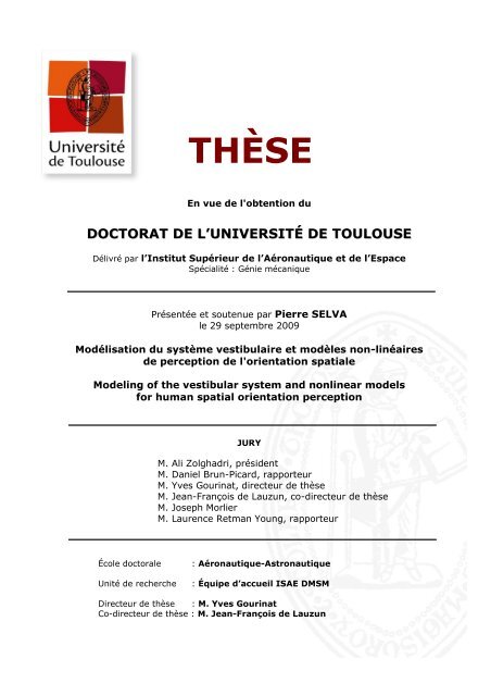
THÈSE<br />
En vue de l'obtention <strong>du</strong><br />
DOCTORAT DE L’UNIVERSITÉ DE TOULOUSE<br />
Délivré par l’Institut Supérieur de l’Aéronautique <strong>et</strong> de l’Espace<br />
Spécialité : Génie mécanique<br />
Présentée <strong>et</strong> soutenue par Pierre SELVA<br />
le 29 septembre 2009<br />
<strong>Modélisation</strong> <strong>du</strong> <strong>système</strong> <strong>vestibulaire</strong> <strong>et</strong> <strong>modèles</strong> <strong>non</strong>-linéaires<br />
de perception de l'orientation spatiale<br />
Modeling of the vestibular system and <strong>non</strong>linear models<br />
for human spatial orientation perception<br />
JURY<br />
M. Ali Zolghadri, président<br />
M. Daniel Brun-Picard, rapporteur<br />
M. Yves Gourinat, directeur de thèse<br />
M. Jean-François de Lauzun, co-directeur de thèse<br />
M. Joseph Morlier<br />
M. Laurence R<strong>et</strong>man Young, rapporteur<br />
École doctorale<br />
Unité de recherche<br />
: Aéronautique-Astronautique<br />
: Équipe d’accueil <strong>ISAE</strong> DMSM<br />
Directeur de thèse : M. Yves Gourinat<br />
Co-directeur de thèse : M. Jean-François de Lauzun
[This page intentionally left blank]<br />
2
ACKNOWLEDGMENTS<br />
I am deeply indebted to my thesis advisors Prof. Yves Gourinat and ENT specialist Jean-François<br />
Delauzun as they always believed in my abilities and provided whatever advice and resources<br />
necessary to accomplish my goals. I learned a lot from our discussions, and your advices were always<br />
wise and most useful.<br />
I am most grateful to Dr. Charles Oman for giving the opportunity to work at the Man Vehicle Lab at<br />
MIT and who made significant contributions to the success of this investigation. Thank you for<br />
providing many invaluable hours me<strong>et</strong>ing to discuss aspects of my research and working revisions of<br />
my various publications.<br />
Tremendous thanks to Associate Prof. Joseph Morlier for guidance and support throughout the last<br />
three years. The willingness to answer questions and help with challenges of all sorts was greatly<br />
appreciated.<br />
My thesis committee, Professor Laurence R. Young and Professor Daniel Brun Picard, deserve special<br />
thanks.<br />
For funding my stay in the US I am grateful to François Prieur. I would not have lived this great<br />
experience without your support. I also thank <strong>ISAE</strong> and MIT for giving me the chance to study in the<br />
US.<br />
To my roommates Annie Park, Jennifer Burger, Kimberley Clark and Yui Kumnerdpun: thank you<br />
guys for all the fun and the time we spent tog<strong>et</strong>her. Thank you Annie for your generosity and<br />
friendship and for always caring for me, MAMA!! Thank you Jen for being an awesome roommate,<br />
for your support, and for improving my English! Kim, you are an amazing person, thank you for the<br />
energy and craziness you brought to the house. Thank you Yui for all the chicken salads and Ronny<br />
burgers we split tog<strong>et</strong>her, and, above all, thank you for all the fun and laugh shared. My thoughts as<br />
well to Christopher O’Keeffe and Christine Newsham, thank you for your generosity and for all the<br />
fun and the time we spent tog<strong>et</strong>her, you guys are awesome. Many thanks to all the other people I m<strong>et</strong><br />
in Cambridge. I really had a great time with all of you guys, you all participated in making my stay in<br />
the US an unforg<strong>et</strong>table story.<br />
Thank you to Liz Zotos for always being so pleasant and helpful with administrative issues.<br />
A lot of people have contributed their time, ideas, feedback and support over the last three years.<br />
Thank you, Michael Newman, Dr. Howard Stone, Dr. Grégoire Casalis, Dr. Dan Merfeld, Faisal<br />
Kamali, Guilhem Michon, Mathieu Bizeul, Amir Shahdin, Damien Guillon, Boris Chermain, Issam<br />
Tawk, Javier Toral Vazquez, Elias Abi Adallah, and all the other labmates and friends who have given<br />
me wonderful advice, inspiration and friendship over the years.<br />
I would like to acknowledge everyone who provided technical support, especially for the zero G flight.<br />
Big thanks to Guy Mirabel, Xavier Foulquier, Marc Chartrou, Joel Xuereb, Thierry Duigou, Marc<br />
Chevalier, and Philippe Fargeout.<br />
To all my friends from Bagnères de Bigorre and Toulouse who have supported and helped me along<br />
the way, and who have given me inspiration and friendship over the years. There are far too many<br />
people to list, but I think you all know who you are.<br />
To my family, your love and support made this possible. You always believed in me and it gave me<br />
the strength to succeed. Mom, Dad, Françoise, Jos<strong>et</strong>te, and Michel, thank you so much.<br />
Last but not least, thank you to “mon coeur”, Mélanie: you have always been with me from the start<br />
and I could never have gone so far without you. When you hold my hands, nothing is out of reach, not<br />
even my dreams.<br />
3
Table of contents<br />
ACKNOWLEDGMENTS .................................................................................. 3<br />
List of figures ....................................................................................................... 7<br />
List of tables......................................................................................................... 9<br />
General intro<strong>du</strong>ction.........................................................................................10<br />
Contributions of this work.................................................................................................... 11<br />
Objectives of the thesis ........................................................................................................ 13<br />
Thesis organization .............................................................................................................. 15<br />
Chapter I: Background.....................................................................................16<br />
1.1. Vestibular physiology ................................................................................................... 16<br />
1.1.1. The semicircular canals.......................................................................................... 17<br />
1.1.2. Otolith organs......................................................................................................... 20<br />
1.2. Mathematical modeling................................................................................................. 21<br />
1.2.1. Semicircular canals ................................................................................................ 21<br />
1.2.2. Otolith organs......................................................................................................... 25<br />
1.3. History of spatial orientation......................................................................................... 28<br />
1.4. State estimation of dynamic state-space models ........................................................... 32<br />
1.4.1. Intro<strong>du</strong>ction ............................................................................................................ 32<br />
1.4.1.1. Probalistic inference........................................................................................ 33<br />
1.4.1.2. Gaussian approximate m<strong>et</strong>hods....................................................................... 33<br />
1.4.2. Linear state space estimation.............................................................................. 34<br />
1.4.2.1. Kalman filtering .............................................................................................. 35<br />
1.4.3. Nonlinear state-space estimation............................................................................ 37<br />
1.4.3.1. Nonlinear transformation of random variables ............................................... 38<br />
1.4.3.2. The extended Kalman filter............................................................................. 42<br />
1.4.3.3. The unscented Kalman filter ........................................................................... 44<br />
Chapter II: Finite element modeling...............................................................50<br />
2.1. Modeling of the cupula ................................................................................................. 50<br />
2.1.1. Background ............................................................................................................ 50<br />
2.1.3. Analytical model using thin and thick bending membrane theory......................... 54<br />
2.1.4. Finite-element models ............................................................................................ 55<br />
2.1.4.1. Computation of the Young’s mo<strong>du</strong>lus ............................................................ 55<br />
2.1.4.2. Comparison with other estimates .................................................................... 57<br />
2.1.4.3. Analysis of different cupula shapes ................................................................ 58<br />
2.1.4.5. Mechanical influence of cupula channels ....................................................... 61<br />
2.1.5. Biologically similar material.................................................................................. 62<br />
2.2. Fluid structural interaction model ............................................................................ 64<br />
2.2.1. Intro<strong>du</strong>ction ............................................................................................................ 64<br />
2.2.2. Fluid-structure interaction ...................................................................................... 64<br />
2.2.3. Arbitrary Lagrangian Eulerian m<strong>et</strong>hodology ......................................................... 65<br />
2.2.4. 2D model ................................................................................................................ 67<br />
2.2.4.1. Geom<strong>et</strong>ry of the 2D model.............................................................................. 67<br />
2.2.4.2. Governing equations ....................................................................................... 68<br />
4
2.2.4.3. Boundary conditions ....................................................................................... 70<br />
2.2.4.4. Moving mesh................................................................................................... 72<br />
2.2.4.5. Simulations...................................................................................................... 73<br />
2.2.5. Three-dimensional model of a single canal............................................................ 79<br />
2.2.6. 3D model of the entire s<strong>et</strong> of canals....................................................................... 81<br />
Chapter III: Virtual reality model...................................................................84<br />
3.1. Virtual reality model ..................................................................................................... 84<br />
3.1.1. Intro<strong>du</strong>ction ............................................................................................................ 84<br />
3.1.2. Formulation of the kinematic problem................................................................... 85<br />
3.1.2.1. Rotation of reference frames ........................................................................... 87<br />
3.1.2.2. Orientation of the SCC coordinate system...................................................... 87<br />
3.1.2.3. Expression of the angular velocity vectors ..................................................... 88<br />
3.1.2.4. Expression of the angular acceleration vector................................................. 89<br />
3.1.2.5. Expression of the linear acceleration vectors.................................................. 90<br />
3.1.3. Programming and implementation ......................................................................... 94<br />
3.1.3.1. Graphical user interface .................................................................................. 94<br />
3.1.3.2. Simulink model ............................................................................................... 95<br />
3.1.3.4. Virtual reality model ....................................................................................... 98<br />
3.1.3.5. Simulation and visualization ........................................................................... 99<br />
3.1.3.6. Conclusion..................................................................................................... 101<br />
Chapter IV: Models for human spatial orientation.....................................102<br />
4.1. Intro<strong>du</strong>ction ................................................................................................................. 102<br />
4.1. Relationships b<strong>et</strong>ween Observer and Kalman filter models for human dynamics spatial<br />
orientation........................................................................................................................... 104<br />
4.1.2. Observer and KF model comparison: yaw rotation in darkness .......................... 104<br />
4.1.2.1. Merfeld 1-D Observer model ........................................................................ 104<br />
4.1.2.2. Borah 1-D Kalman filter model .................................................................... 105<br />
4.1.2.3. Ecologic basis for 1-D Kalman filter model param<strong>et</strong>ers............................... 107<br />
4.1.3. Observer and KF 3-D model for somatogravic illusion in darkness.................... 109<br />
4.1.3.1. Three-dimensional Merfeld Observer model for large tilts .......................... 110<br />
4.1.3.2. Three-dimensional Borah steady state Kalman filter for small tilts.............. 111<br />
4.2. Nonlinear models for human spatial orientation based on the hybrid extended and<br />
unscented Kalman filter ..................................................................................................... 117<br />
4.2.1. Coordinate system ................................................................................................ 117<br />
4.2.2. Modeling of the sensors ....................................................................................... 118<br />
4.2.3. Description of the model ...................................................................................... 119<br />
4.2.3.1. Real world model .......................................................................................... 120<br />
4.2.3.2. Internal model of the CNS ............................................................................ 121<br />
4.2.4. Estimation process................................................................................................ 122<br />
4.2.4.1 State vector update ......................................................................................... 122<br />
4.2.4.2. Measurement equations: outputs of the real world model ............................ 127<br />
4.2.5. Implementation consideration .............................................................................. 128<br />
4.2.6. Simulation results................................................................................................. 129<br />
4.2.6.1. Param<strong>et</strong>ers ..................................................................................................... 129<br />
4.2.6.2. Constant velocity rotation about an earth vertical axis ................................. 130<br />
4.2.6.3. Forward linear acceleration in darkness........................................................ 133<br />
4.2.6.4. Vestibular “Coriolis” Cross-coupling ........................................................... 134<br />
4.2.6.5. Pseudo-Coriolis illusion ................................................................................ 136<br />
5
4.2.7 Sensitivity study .................................................................................................... 138<br />
4.2.7.1. Yaw angular velocity in darkness ................................................................. 138<br />
4.2.7.2. Forward linear acceleration in darkness........................................................ 139<br />
4.2.7.3. Vestibular Coriolis illusion ........................................................................... 142<br />
Chapter 5. Scale model of the semicircular canals ......................................143<br />
5.1. Similitude study........................................................................................................... 143<br />
5.2. Choice of materials...................................................................................................... 147<br />
5.3. Results ......................................................................................................................... 148<br />
Chapter 6. Conclusion and future works......................................................150<br />
6.1. Overall conclusion....................................................................................................... 150<br />
6.2. Perspectives................................................................................................................. 154<br />
References ........................................................................................................156<br />
Appendix 1:......................................................................................................163<br />
Numerical model for the resolution of the fluid flow within a single canal<br />
...........................................................................................................................163<br />
Appendix 2: Quaternions and spatial rotation.............................................171<br />
Appendix 3: Example of Simulink model used to generate sensors output<br />
for motion paradigms in darkness.................................................................172<br />
Appendix 4: EKF and UKF models: Matlab code.......................................173<br />
6
List of figures<br />
Figure 1.1. Visualization of the inner ear.<br />
Figure 1.2. Orientation of the semicircular canals.<br />
Figure 1.3. Cross-section of the ampulla and functioning of the hair cells.<br />
Figure 1.4. D<strong>et</strong>ection of an angular acceleration of the SCC through inertia of the endolymph fluid<br />
relative to the canal motion.<br />
Figure 1.5. Physiology of the utricular macula.<br />
Figure 1.6. Mechanism of the otolith organs, showing their sensitivity to linear acceleration and head<br />
tilt.<br />
Figure 1.7. Mechanical model of a semicircular canal.<br />
Figure 1.8. Curve of typical cupula displacement and Bode diagram of the transfer function b<strong>et</strong>ween<br />
head angular velocity and cupula displacement.<br />
Figure 1.9. Schematic diagram of the functioning of the Otolith organs.<br />
Figure 1.10. Borah <strong>et</strong> al. multisensory model using steady state Kalman filter to represent neural<br />
central processing.<br />
Figure 1.11. Outline of the three-dimensional model of Merfeld.<br />
Figure 1.12. Principle of human spatial orientation estimation model.<br />
Figure 1.13. Demonstration of the accuracy of the unscented transformation for mean and covariance<br />
propagation.<br />
Figure 2.1. Three-dimensional model of the cupula.<br />
Figure 2.2. Transversal displacement w( r)<br />
provided by the thin and thick analytical membrane<br />
models, and the finite element circular plate model.<br />
Figure 2.3. Top view of the skate cupula which is thicker on the sides and thin in the center.<br />
Figure 2.4. CAD models of the cupula considering different shapes.<br />
Figure 2.5. Transversal displacement of the human cupula provided by a finite element simulation in<br />
response to a static pressure of 0.05 Pa.<br />
Figure 2.6. Analysis of the shear strain above the crista.<br />
Figure 2.7. Modeling of a section of cupula material having vertical empty tubes<br />
Figure 2.8. Results provided by the finite-element model of a section of cupula material having<br />
vertical empty tubes.<br />
Figure 2.9. Representative frequency sweeps of G’ and G’’ for collagen hydrogels at each<br />
polymerization temperature.<br />
Figure 2.10. Comparison Lagrangian and Eulerian descriptions. 2D example of a beam that undergoes<br />
a pressure P .<br />
Figure 2.11. Comparison Lagrangian, Eulerian, and ALE descriptions<br />
Figure 2.12. Dimensions of the human lateral semicircular canal and reconstruction of a 2D model<br />
under Comsol Multiphysics.<br />
Figure 2.13. Concept of fluid-structure interaction (FSI).<br />
Figure 2.14. Smoothed Heaviside function flc2 hs( t −t0, ∆t)<br />
with a continuous second derivative<br />
Figure 2.15. Visualization of the subdomains that have different conditions for mesh displacement.<br />
Figure 2.16. Rotational motion applied to the semicircular canal.<br />
Figure 2.17. Evolution of the displacement of the cupula at the very beginning of the imposed<br />
rotational motion.<br />
Figure 2.18. Evolution of the velocity of the fluid in the slender part of the <strong>du</strong>ct at the beginning of the<br />
rotational motion.<br />
Figure 2.19. Fluid velocity and cupula displacement at the beginning of the rotation. Visualization in<br />
the ALE reference frame.<br />
Figure 2.20. Fluid velocity and cupula displacement at the end of the rotation. Visualization in the<br />
ALE reference frame.<br />
Figure 2.21. Displacement of the center of the cupula <strong>du</strong>ring a constant angular rotation which ends at<br />
time t=15 s.<br />
7
Figure 2.22. Rotation of the canal located 30 mm away from the axis of rotation. The arrows are<br />
oriented along the fluid flow.<br />
Figure 2.23. Visualization of a three-dimensional single canal.<br />
Figure 2.24. Fluid velocity in m/s and cupula displacement in m at time instant t=0.03 s and t=1 s.<br />
Figure 2.25. Three-dimensional CAD model of the three SCCs + utricle +cupulae.<br />
Figure 2.26. Mesh of the final three-dimensional model which consists of 111 quadratics elements<br />
that represents 111 degrees of freedom.<br />
Figure 2.27. Results provided by the simulation of the final 3D model of the semicircular canals.<br />
Figure 3.1. Schematic block diagram of the virtual reality simulink model<br />
Figure 3.2. Visualization of the diagnosis proce<strong>du</strong>re and definition of the different coordinate systems<br />
Figure 3.3. Definition of head movements: pitch, roll, and yaw.<br />
Figure 3.4. Orientation of the coordinate systems for a yaw head movement while the subject is<br />
rotated around an Earth vertical axis.<br />
Figure 3.5. Orientation of the coordinate systems for a pitch head movement while the subject is<br />
rotated around an Earth vertical axis.<br />
Figure 3.6. Orientation of the coordinate systems for a roll head movement while the subject is rotated<br />
around an Earth vertical axis.<br />
Figure 3.7. Graphical user interface of the virtual reality model<br />
Figure 3.8. First layer of the simulink model.<br />
Figure 3.9. D<strong>et</strong>ailed view of the block of the first layer titled “SCC”.<br />
Figure 3.10. D<strong>et</strong>ailed view of the block of the first layer titled “utricle-saccule”.<br />
Figure 3.11. Schematic block diagram of how the virtual reality world is created and controlled..<br />
Figure 3.12. Displacement of the cupula of each canal <strong>du</strong>e to rotation movement of the chair, and<br />
rotation movement of the chair and of the head<br />
Figure 3.13. Visualization of a virtual scene: The state of each sensor can be visualized on real time<br />
<strong>du</strong>ring the test.<br />
Figure 4.1. Principle outline of the internal model concept applied for the estimation of external<br />
physical variables like acceleration, velocity, and position.<br />
Figure 4.2. Merfeld Observer model for a yaw rotation.<br />
Figure 4.3. Merfeld Observer model showing pole/zero cancellation.<br />
Figure 4.4. One-dimensional Borah’s Kalman filter model.<br />
Figure 4.5. Kalman filter model for yaw rotation (left)<br />
Figure 4.6. Observer and KF estimated angular velocity responses to a 100 deg/s angular velocity<br />
step.<br />
Figure 4.7. Kalman gain K 21 with respect to Q / V ratio and shaping filter bandwidth.<br />
Figure 4.8. Somatogravic illusion.<br />
Figure 4.9. 3D Observer model.<br />
Figure 4.10. 3D internal model used in the present Kalman filter model.<br />
Figure 4.11. Block diagram of the steady state Kalman filter for the somatogravic illusion.<br />
Figure 4.12. Perception of linear acceleration and pitch angle in response to a forward linear acceleration of<br />
0.2g provided by Merfeld Observer and Kalman filter model.<br />
Figure 4.13. Perception of linear acceleration and pitch angle in response to a forward linear acceleration of<br />
0.2g provided by the Kalman filter model for two different otolith dynamics.<br />
Figure 4.14. Response of the Kalman filter model with Borah’s otolith transfer function for different bandwiths<br />
of linear acceleration<br />
Figure 4.15. Head and world coordinate frame.<br />
Figure 4.16. Coordinate system attached to the sensors<br />
Figure 4.17. Sensors transfer functions used in the EKF and UKF models.<br />
Figure 4.18. Philosophy of the <strong>non</strong>linear model of human spatial orientation perception.<br />
Figure 4.19. D<strong>et</strong>ailed view of the model of the real world<br />
Figure 4.20. D<strong>et</strong>ailed view of the model of the internal model of the CNS<br />
Figure 4.21. Equivalent model of the low pass filter<br />
Figure 4.22. Equivalent representation of the transfer functions of the semicircular canal dynamics.<br />
Figure 4.23. Equivalent representation of the transfer functions of the otolith dynamics.<br />
Figure 4.24. Graphical user interface of the EKF/UKF models.<br />
Figure 4.25. Scheme of the yaw rotation experiment in darkness.<br />
8
Figure 4.26. Model response to a step in yaw angular velocity.<br />
Figure 4.27. Model response to a step in yaw angular velocity of the surrounding environment.<br />
Figure 4.28. Model response to a step in forward linear acceleration of 2 m/s<br />
Figure 4.29. Description of the Coriolis illusion.<br />
Figure 4.30. Simulation of vestibular Coriolis effect I<br />
Figure 4.31. Simulation of vestibular Coriolis effect II<br />
Figure 4.32. Description of the pseudo-Coriolis illusion.<br />
Figure 4.33. Simulation of the pseudo-Coriolis illusion.<br />
Figure 4.34. Influence of the bandwidth in angular velocity on the estimated yaw angular velocity in darkness.<br />
Figure 4.35. Influence of the bandwidth in linear acceleration on the estimated linear acceleration (a) and<br />
perceived pitch angle (b) in darkness.<br />
Figure 4.36. Influence of the linear acceleration process noise on the estimated linear acceleration (a) and<br />
perceived pitch angle (b)in response to a forward acceleration in darkness.<br />
Figure 4.37. Influence of bandwidth in head angular velocity on the estimated yaw angular velocity (a) and<br />
perceived pitch angle (b) in response to a Coriolis stimulation in darkness.<br />
List of tables<br />
Table 1.1. Validation cases for Observer and KF / EKF models<br />
Table 2.1. Summary of the values of the pressure-volume coefficient along with its relation to the long<br />
time constant of the cupula. See nomenclature for definition of param<strong>et</strong>ers.<br />
Table 2.2. Relationship b<strong>et</strong>ween the Young’s mo<strong>du</strong>lus of the cupula and the pressure-volume<br />
coefficient K.<br />
Table 2.3. Expression of the prescribed displacements for a head rotation.<br />
Table 2.4. Boundary conditions of the two-dimensional finite-element model of the horizontal<br />
semicircular canal.<br />
Table 5.1. Dimension of the physical param<strong>et</strong>ers that influences fluid flow within a semicircular canal<br />
in terms of fundamental units.<br />
Table 5.2. Matrix form of the Buckingham Pi theorem.<br />
Table 5.3. Matrix form of the Buckingham Pi theorem applied to our similitude problem.<br />
Table 5.4. Required experimental values for cupula material Young’s mo<strong>du</strong>lus and maximum<br />
simulated head angular velocity<br />
Table 5.5. Quantitative estimation of possible configurations that keep constant all the dimensionless<br />
param<strong>et</strong>ers.<br />
Table 6.1. Summary of the sensitivity study of some of the param<strong>et</strong>ers of the UKF model.<br />
9
General intro<strong>du</strong>ction<br />
Daily human activity includes complex orientation, postural control, and movement<br />
coordination. All these tasks depend upon his perception of motion. The <strong>non</strong>-auditory section<br />
of the human inner ear, the vestibular system, is recognized as the prime motion sensing<br />
center. It represents an inertial measuring device which allows us to sense, in the absence of<br />
external sensory cues (vision, <strong>et</strong>c) self-motion with respect to the six degrees of freedom in<br />
space (three rotational and three translational).<br />
The information from the vestibular apparatus is used in three ways:<br />
• To provide a subjective sensation of movement in three-dimensional space<br />
• To maintain upright body posture (balance)<br />
• To control the muscles that move the eyes, so that in spite of the changes in head<br />
position which occur <strong>du</strong>ring normal activities such as walking or running, the eyes<br />
remain stabilized on a point in space.<br />
Several scenarios illustrate these points. For instance, if a cat is dropped upside down, it will<br />
land right side up on all four paws. If a newborn infant is tilted backward, its eyes will roll<br />
downward so that its gaze remains fixed on the same point. If, as you read this report, you<br />
shake your head rapidly from side to side, the print <strong>non</strong><strong>et</strong>heless will stand still. Each of these<br />
scenarios is an example of how a healthy balance (vestibular) system compensates for daily<br />
changes in our spatial orientation.<br />
The vestibular system is comprised of two primary sense organs:<br />
• The semicircular canals (SCCs), which d<strong>et</strong>ect angular accelerations of the head<br />
• The otolith organs, which respond to linear accelerations of the head and to gravity.<br />
Thus, vestibular sensors provide information to the brain regarding our body’s position and<br />
acceleration in space with sensing capabilities that are compatible with everyday movements<br />
of man relative to his surroundings, and hence play central role in spatial orientation.<br />
Spatial orientation can be defined as one’s perception of body position in relation to a<br />
reference frame. This process involves two main sensory modalities, the vestibular system<br />
and vision, but proprioceptive and auditory inputs also come into play. The control of spatial<br />
orientation <strong>du</strong>ring navigational tasks and locomotion requires a dynamic updating of the<br />
representation of the relations b<strong>et</strong>ween the body and the environment, i.e. spatial orientation<br />
normally entails both the subconscious integration of multisensory cues and the conscious<br />
interpr<strong>et</strong>ation of external information. Therefore, the Central Nervous System (CNS) uses<br />
information coming from multiple sensors to come up with a representation of how the body<br />
is moving and is oriented in space.<br />
The results of this “spatial orientation” process are usually satisfactory in most everyday life<br />
situations. However, when technology achievements began to expose humans to new and<br />
artificial situations such as sustained accelerations in fighter airplanes or micro-gravity<br />
environment in spacecrafts, our ability to correctly estimate our position and motion became<br />
10
limited. As a matter of fact, as the number of fighter airplane accidents <strong>du</strong>e to technical failure<br />
keeps decreasing, human errors have been proven to be a saf<strong>et</strong>y limiting factor. That is, the<br />
advent of aeronautics flight has not only involved a new demand on human organism but also<br />
the ability for pilots to deal with a high workload environment and a complex instrument<br />
panel. Furthermore, in some circumstances, for instance when flying in clouds or at night,<br />
pilots may not have the possibility of seeing external references. As a result, pilots are<br />
constantly liable to intro<strong>du</strong>ce conflict b<strong>et</strong>ween their internal feeling of orientation and the true<br />
orientation, and hence to experience a case of spatial disorientation which is a phenome<strong>non</strong><br />
attributed to 15 to 30% of all aircraft fatalities in flight (Braithwaite <strong>et</strong> al. 1998, Knapp <strong>et</strong> al.<br />
1996). Thus, all these considerations have lead number of researchers to model human spatial<br />
orientation.<br />
Mathematical models for three-dimensional human spatial orientation have continued to<br />
evolve over the past four decades. Several models exist and have been developed using<br />
multiple computational approaches such as linear systems analysis, the concept of internal<br />
models, observer theory, Bayesian theory, Kalman filtering and particle filtering. A review of<br />
these approaches has recently been written by MacNeilage (2008). Different features can be<br />
distinguished among these models: some of them are restricted to one-dimensional space,<br />
whereas others take into account motions in three-dimensional space; some incorporate visual<br />
cues, whereas others only model vestibular response in the dark; and some work for large<br />
head tilts whereas others do not.<br />
Contributions of this work<br />
The scope of the work presented in this thesis concerns on one hand the modeling of the<br />
vestibular sensors, and more particularly the semicircular canals, and on the other hand<br />
<strong>non</strong>linear models for human spatial orientation perception.<br />
Since the 30’s, numerous models of the semicircular canal macromechanics have been<br />
suggested using different approaches. W. Steinhausen (1933) formulated a classical torsion<br />
pen<strong>du</strong>lum model for the dynamic behavior of a single SCC. This model, which has been the<br />
benchmark for subsequent works, consists of a single-degree of freedom overdamped springmass-damper<br />
system subject to mass-proportional inertia forcing. Several notable extensions<br />
have then been made to enhance this original model by relating the geom<strong>et</strong>ry and structure of<br />
the SCC to mass, stiffness, and damping param<strong>et</strong>ers appearing in the model (e.g. Van<br />
Egmond <strong>et</strong> al. 1949, Groen <strong>et</strong> al. 1952, Van Buskirk 1976, Oman <strong>et</strong> al. 1987, Rabbitt <strong>et</strong> al<br />
2004). Other models were based on the resolution of the fluid flow equation within the canal<br />
(Van Buskirk 1977, Van Buskirk 1988, Steer 1967, Oman <strong>et</strong> al. 1987, Damiano <strong>et</strong> al. 1996,<br />
Rabbitt <strong>et</strong> al. 1999). The three-dimensional model of Oman <strong>et</strong> al. (1987), in which the <strong>non</strong>uniform<br />
geom<strong>et</strong>ry of the canal was considered, probably constitutes the most compatible<br />
biophysical single-degree of freedom model of the SCC. Some of these models are formulated<br />
in one dimension, while few of them consider a three-dimensional geom<strong>et</strong>ry. Moreover, all of<br />
these models consider a single canal and most of them do not take into account the fluidstructure<br />
interaction but rather consider the influence of the cupula by a punctual elasticity.<br />
Therefore, the first goal of the present thesis is to provide a three-dimensional model of<br />
the entire s<strong>et</strong> of canals using fluid-structural finite-elements simulations. To achieve this goal,<br />
we first develop a two dimensional finite-elements model of a single canal. Second, this<br />
11
model is extended to a three-dimensional case. Finally, the 3D model is extended to the case<br />
where the three semicircular canals are considered.<br />
In order to build these numerical models, one needs to know the physical properties of the<br />
fluid that fills the canals and the elastic properties of the cupula - a membrane located within<br />
the <strong>du</strong>ct that acts as a coupling b<strong>et</strong>ween the fluid flow and sensory hair cells. The properties<br />
of the fluid, i.e. its density and viscosity, are well known (Steer, 1967). However, it is hard to<br />
find in the literature values for the elastic properties of the human semicircular canal cupula,<br />
and more especially its Young’s mo<strong>du</strong>lus, as most model represent the cupula as a linear<br />
spring-like element of stiffness K = ∆P / ∆ V ,where ∆ V is the volume displaced upon<br />
application of a pressure difference ∆ P .<br />
Thus, the second goal of this doctoral work is to estimate the Young’s mo<strong>du</strong>lus of the<br />
human semicircular canal cupula using thick plate theory and also finite-elements (FE)<br />
models. In addition, cupula FE models are also used to study the influence of different cupula<br />
shapes on its motion and to analyse both the shear strain distribution and evolution near the<br />
sensory epithelium.<br />
As we move in our surrounding in space, our vestibular sensors provide information to the<br />
brain regarding our body’s position and acceleration in space. However, the way each sensor<br />
behaves for any angular or linear acceleration is not obvious, especially for complex head<br />
motion. In particular, in order to find out what are the semicircular canals sensing when a<br />
subject is doing head movements on a centrifuge Adenot (2002) developed a model that was<br />
able to compute the state of each cupula <strong>du</strong>ring the imposed motion. However, this model was<br />
limited to SCC sensors, considered a head centered s<strong>et</strong> of sensors, and the implementation of<br />
successive head movements was not possible.<br />
Consequently, the third goal of this thesis is to extend this model: 1) by considering not<br />
only the angular but also the linear sensors, 2) by taking into account the position of the inner<br />
ear away from head vertical axis, 3) by implementing a three-dimensional animation of the<br />
sensors, and 4) by developing a virtual reality model of the experiment. As an application, we<br />
have chosen to model a medical proce<strong>du</strong>re called the rotary chair testing that is commonly<br />
used <strong>du</strong>ring a vestibular diagnosis rather than a centrifuge experiment. However, the<br />
developed model can be easily extended to the case of a centrifuge paradigm as the distance<br />
b<strong>et</strong>ween the position of the inner ear and the axis of rotation is a param<strong>et</strong>er of the model.<br />
In addition to this virtual model, we propose a similitude study, a choice of adequate<br />
materials, and a s<strong>et</strong> of param<strong>et</strong>ers so as to build a large scale model of the system SCC /<br />
cupula that has a similar dynamic behavior of the biological system for a specific imposed<br />
angular velocity.. Both models (virtual and scale model) can be used as a demonstrating and<br />
learning tool, for instance for the training of medical students, as the theor<strong>et</strong>ical state of each<br />
sensor can be observed in real time for any kind of head rotation.<br />
Regarding to the models of human spatial orientation, two principle model families can be<br />
distinguished: Observer class models and Kalman filter class models. Although both<br />
approaches are apparently based on different assumptions, they pro<strong>du</strong>ce similar responses, at<br />
least for the s<strong>et</strong> of empirical param<strong>et</strong>ers derived in the literature.<br />
12
The fourth goal of this thesis is to demonstrate why the Observer and Kalman filter<br />
model families are dynamically equivalent from an input-ouput perspective. Furthermore, we<br />
investigate the physical meaning of the KF model param<strong>et</strong>ers that were previously chosen as<br />
free param<strong>et</strong>er of the model and were derived empirically.<br />
The first Observer model developed by Merfeld <strong>et</strong> al. (1993) has then been extended by<br />
several authors till the last contributions of Newman (2009). Despite this model is able to<br />
simulate different kinds of sensory illusions, it is limited to d<strong>et</strong>erministic signals as it does not<br />
consider process noise and sensor noise. Furthermore, the gains used in the model that drive<br />
the responses in term of position, velocity, and acceleration perception are empirical. In order<br />
to derive a s<strong>et</strong> of optimal gains and to take into consideration stochastic signals, Pommell<strong>et</strong><br />
(1990) applied the extended Kalman filter (EKF) to this problem. However, his filter<br />
exhibited important numerical oscillations.<br />
Therefore, the fifth goal of this thesis is first to modify Pommell<strong>et</strong>’s model so as to<br />
improve numerical stability and second to develop another <strong>non</strong>linear model based on a novel<br />
estimation technique called the unscented Kalman filter (UKF). It has been shown that in<br />
many applications this technique outperforms the EKF in terms of stability, accuracy, and<br />
computation time.<br />
Objectives of the thesis<br />
The main objectives of the presented thesis are summarized as follows:<br />
• Estimation of the elastic properties of the human semicircular canal cupula – a<br />
membrane located in each canal that functions as a coupling b<strong>et</strong>ween the fluid flow<br />
within the <strong>du</strong>cts and the sensory hair cells –using thin and thick bending membrane<br />
theory and also finite-element simulations based on more realistic morphology<br />
• Develop of a three-dimensional model of the s<strong>et</strong> of semicircular canals based on fluidstructural<br />
finite-elements simulations<br />
• Develop of a three-dimensional dynamic virtual reality model of the vestibular sensors<br />
in order to propose both a demonstrating and a learning tool of this system<br />
• Propose a similitude study so as to build a large scale model of the semicircular canals<br />
• Demonstrate why the widely known “Observer” and “Kalman filter” model families<br />
for human spatial orientation perception – despite apparently different assumptions –<br />
are dynamically equivalent from an input-output (“black box”) perspective<br />
• Develop two <strong>non</strong>linear models for human spatial orientation estimation with the help<br />
of the extended Kalman filter and the unscented Kalman filter, respectively. Both<br />
models are formulated in three-dimensional space and take into account vestibular and<br />
visual cues.<br />
13
Based on the work of this thesis, the author has so far succeeded in publishing the following<br />
works:<br />
• International peer-reviewed journals:<br />
Development of a dynamic virtual reality model of the inner ear sensory<br />
system as a learning and demonstrating tool. Modelling and Simulation in<br />
Engineering, volume 2009.<br />
• International conference with proceedings:<br />
A Matlab/simulink model of the inner ear angular accelerom<strong>et</strong>ers sensors.<br />
ASME, International Design Engineering Technical Conferences & Computers<br />
and Information in Engineering Conference, August 30 – September 2 nd , San<br />
Diego, California, USA.<br />
• Manuscripts under progress:<br />
Mechanical properties and motion of the cupula of the human semicircular<br />
canal. Journal of Vestibular Research.<br />
Relationship b<strong>et</strong>ween Observer and Kalman filter models for human dynamic<br />
spatial orientation. Journal of Neurophysiology.<br />
Nonlinear models for human spatial orientation. Journal of Biology<br />
Cybern<strong>et</strong>ics.<br />
A three-dimensional finite-element model of the human semicircular canals.<br />
Computer Modeling in Engineering & Sciences.<br />
14
Thesis organization<br />
The presented thesis is organized in six chapters.<br />
• Chapter 1. – Background: Provides a background on the anatomy and physiology of<br />
the vestibular system, on the history of spatial orientation modeling, and on state<br />
estimation techniques of dynamic state-space models.<br />
• Chapter 2. – Finite element modeling: Presents finite-element models for the cupula<br />
and finite-element fluid-structural interaction model of the semicircular canals.<br />
Intro<strong>du</strong>ces the history on cupula attachment, bending mode, stiffness, and modeling.<br />
Estimates the Young’s mo<strong>du</strong>lus of the cupula using thin and thick bending membrane<br />
theory, finite-element simulations, and estimates of a pressure-volume coefficient<br />
taken from the literature. Presents a three-dimensional finite-element model of the<br />
semicircular canals.<br />
• Chapter 3. – Virtual reality model: Presents the development of a virtual reality model<br />
of the vestibular sensors. The kinematics problem is first formulated. The resolution of<br />
the equation of motions and the computation of the state of each sensor are achieved<br />
using a Simulink model. Finally, a virtual world is linked to the Simulink file so as to<br />
visualize in real time the behavior of the sensory system. Note that a graphic user<br />
interface is specifically developed to simplify the use of the model.<br />
• Chapter 4. – Models for human spatial orientation perception: Demonstrates why the<br />
“Observer” and “Kalman filter” model families are equivalent from an input-output<br />
perspective. Intro<strong>du</strong>ces the idea that the motion disturbance and sensor noise spectra<br />
employed in the Kalman Filter formulation may reflect human perceptual thresholds<br />
and prior motion exposure history. Describes the structure of the EKF and UKF<br />
models through the modeling of the sensors and the definition of the central process in<br />
terms of suboptimal estimation. Discusses implementation in Matlab. Presents<br />
predictions of the model for usual experimental cases. Performs a sensitivity analysis<br />
on the param<strong>et</strong>ers of the model.<br />
• Chapter 5. – Scale model of the semicircular canals: a similitude study for the<br />
semicircular canal is presented, and potential materials for the manufacturing of the<br />
large scale model are proposed.<br />
• Chapter 6. – Conclusion: Summarizes the key findings of this study and makes<br />
recommendations for future work.<br />
The work related to the development of models for human spatial orientation estimation and<br />
to finite-elements modeling of the cupula has been carried out while the author was a visiting<br />
student at Massachus<strong>et</strong>ts Institute of Technology.<br />
15
Chapter I: Background<br />
1.1. Vestibular physiology<br />
The inner ear is divided into two parts: the cochlea serving auditory function, and the<br />
vestibular system - which is phylogen<strong>et</strong>ically the oldest part of the inner ear - that contains the<br />
sensors providing information of body orientation and balance in three-dimensional space.<br />
Any motion of the body are thus d<strong>et</strong>ected by the vestibular system, encoded as an electrical<br />
signal, and transmitted to the brain through the vestibular nerve. The brain then integrates<br />
vestibular, visual, and somatosensory inputs to estimate the orientation and motion of the<br />
body, and consequently elicit eye, head, or body movements that will stabilize gaze and<br />
maintain balance.<br />
There is one vestibular system on each side of the head, in close approximation to the cochlea.<br />
Due to its specific structure, this system is also called the labyrinth (Fig. 1.1). One<br />
distinguishes b<strong>et</strong>ween the bony labyrinth and the membranous labyrinth. The bony labyrinth<br />
is a complex cavity tunneled in the temporal bone of the skull. Its structure forms three <strong>du</strong>cts -<br />
the semicircular canals - that converge toward a larger central part called “the vestibule”. The<br />
membranous labyrinth is enclosed in this osseous labyrinth, and is suspended in a fluid called<br />
“the perilymph” (Sauvage, 1999). In birds and mammals, fine connective tissue filaments<br />
suspend the membranous <strong>du</strong>ct within the osseous canal. The filaments serve to anchor the<br />
membranous labyrinth to the temporal bone such that the gravitoinertial acceleration<br />
experienced by the sensory organs could be expected to be nearly identical to that experienced<br />
by the temporal bone. To date, there are no experimental data to suggest significant relative<br />
motion b<strong>et</strong>ween the temporal bone and the membranous labyrinth (Rabbitt, 2004). The<br />
membranous labyrinth is also filled with fluid known as “the endolymph”, physically a waterlike<br />
liquid. Each side of this bilateral system consists of two types of sensors: a s<strong>et</strong> of three<br />
semicircular canals sensing rotation movement, and two otolith organs (the saccule and<br />
utricle) which sense linear movement and head tilt.<br />
Inner ear<br />
Vestibular<br />
system<br />
cochlea<br />
Vestibular nerve<br />
2<br />
1<br />
4<br />
7<br />
8<br />
3 5 6<br />
ear canal<br />
stapes<br />
malleus<br />
ear drum<br />
Middle<br />
ear<br />
4<br />
Outer ear<br />
Figure 1.1. Visualization of the inner ear. 1) Anterior canal, 2) posterior canal, 3) lateral canal, 4) ampulla of<br />
each canal, 5) common crux, 6) utricle, 7) saccule, 8) cochlea.<br />
16
1.1.1. The semicircular canals<br />
The semicircular canals are commonly referred to as the lateral canal, also called horizontal<br />
canal, and the posterior and anterior canals, which constitutes the vertical canals. These latter<br />
have a common <strong>du</strong>ct called the common crux for about 15% of their length. The canals are<br />
oriented in almost mutually orthogonal planes. The lateral canal lies in a plane elevated about<br />
30 degrees from the horizontal plane, while the two others are arranged in diagonal planes<br />
which subtend roughly 45 degrees relative to the frontal and saggital planes of the skull (Fig.<br />
1.2a). Thus, the anterior canal on one side of the head is parallel to the posterior canal on the<br />
other and vice versa, whereas the horizontal canals of both inner ears lie in the same plane.<br />
Because most head movements are not in a single SCC plane, and also because of the<br />
imperfect orthogonality of the three canals, the labyrinth usually resolves a given head<br />
rotation into three components. That is, endolymph motion in each canal measures<br />
component of the head’s rotational velocity in the plane of that canal (Fig. 1.2b). It has also<br />
been shown that each canal admits a specific direction of stimulation, which maximizes the<br />
excitation: the lateral, anterior and posterior canals primarily sense yaw, roll and pitch<br />
respectively (Rabbitt, 1999).<br />
The s<strong>et</strong> of canals constitute a very small fluid-filled system the size of a pea. They<br />
approximately form a circular path of 3.2 mm radius and have a cross section radius along<br />
their slender part of about 0.16mm (Curthoys <strong>et</strong> al., 1987). The study of Curthoys and Oman<br />
probably constitutes the most thorough investigation concerning the dimensions of the human<br />
semicircular canals. From microdissected specimens, they were able to provide measurements<br />
of the sizes, cross-sectional shapes and areas all around the path of fluid flow through the<br />
horizontal semicircular <strong>du</strong>ct, ampulla, and utricle. The results of this study are presented in<br />
more d<strong>et</strong>ail in Chapter II.<br />
At one location in each canal, and more precisely in the vicinity of the utricle, the canal cavity<br />
swells to form a bulbous expansion known as the ampulla that contains a transverse ridge of<br />
sensory epithelium, the crista. The epithelial surface of the crista contains thousands of<br />
sensory hair cells and surrounding supporting cells (Fig. 1.3). Hair cells and supporting cells<br />
are found not only atop the ridge (crest) of the crista, but also down its sloping flanks. Hair<br />
cell sensory cilia project a short distance into tiny channels in the cupula, a gelatinous<br />
structure that extend upward from the surface of the crista all the way to the vault (roof) of the<br />
ampulla. The channels in the cupula material may be created as cupula material is secr<strong>et</strong>ed<br />
upwards from the supporting cells surrounding the each hair cell. The cupula effectively<br />
forms a thick diaphragm that compl<strong>et</strong>ely occludes the canal lumen above the crista, and<br />
covers the entire sensory surface on the crest and both flanks. As d<strong>et</strong>ailed later, it is now<br />
believed that the cupula appears attached to the ampulla around its entire periphery.<br />
When the head is subjected to an angular acceleration, endolymph inertia creates a hydrostatic<br />
pressure that deforms the cupula (Fig. 1.4). Bending of hair cell stereocilia then initiates a<br />
complex trans<strong>du</strong>ction process in hair cells and vestibular afferent neurons. The nervous signal<br />
is finally transmitted to the brain and a sensation of motion results. At a constant rotation rate,<br />
the endolymph in the canals tends to catch up with the rotation of the head <strong>du</strong>e to the<br />
viscosity, eliminating the relative movement. Eventually, as long as the rotation rate remains<br />
constant, the cupula r<strong>et</strong>urns to a vertical position <strong>du</strong>e to its elastic properties and the sensation<br />
of motion eventually ceases.<br />
17
(a)<br />
(b)<br />
(c)<br />
Decomposition of head’s angular<br />
velocity V on to canal axis<br />
Figure 1.2. Orientation of the semicircular canals. (a) Orientation of the semicircular canals within the head.<br />
(b) Definition of canal axis. (c) Resolving head’s angular rotation into vector components. HC, horizontal canal;<br />
RA and LA, right and left anterior canal, respectively; RP and LP, right and left posterior canal, respectively.<br />
All of the hair cells on a semicircular canal crista are oriented or “polarized” in the same<br />
direction. Their stereocilia all have the tall ends pointing the same way. As a result,<br />
endolymph motion that is excitatory for one hair cell will be excitatory for all of the hair cells<br />
on that crista. Horizontal and vertical canals have different direction of polarization. Hair cells<br />
in the horizontal canals are polarized to be excited by flow of endolymph toward the ampulla,<br />
whereas hair cells in the vertical canals are polarized to be excited by flow of endolymph<br />
away from the ampulla.<br />
Experimental studies (e.g. Goldberg and Fernandez, 1971) have shown that afferent neurons<br />
exhibit slightly different dynamics in response to the same head angular acceleration stimulus.<br />
All neurons seem to show a response component proportional to cupula volume displacement,<br />
as estimated from fluid mechanical models. Differences b<strong>et</strong>ween units in static sensitivity,<br />
rate sensitivity and adaptive characteristics are attributed to the hair cell trans<strong>du</strong>ction or<br />
afferent encoding processes.<br />
18
(a)<br />
Vestibular system<br />
(b)<br />
Section of ampulla<br />
(c)<br />
Cupula+crest<br />
cupula<br />
Vestibular nerve ampulla<br />
(d)<br />
Excitation<br />
(depolarize)<br />
Resting<br />
Inhibition<br />
(hyperpolarize)<br />
Hair cell<br />
Hair cell<br />
direction of excitation<br />
(polarization)<br />
Vestibular afferent<br />
discharge rate<br />
crista<br />
Figure 1.3. Cross-section of the ampulla and functioning of the hair cells. (a) Visualization of the vestibular<br />
system; (b) Section of ampulla showing how the cupula seals the <strong>du</strong>ct; (c) D<strong>et</strong>ails of the crista and hair cells<br />
implantation; (d) Function of vestibular hair cells: when mechanical forces deviate the cilia toward the<br />
kinocilium, the hair cell depolarizes and the frequency of action potentials in the associated afferent vestibular<br />
neurons increases. When the cilia are deviated in the opposite direction, the hair cell hyperpolarizes and the<br />
frequency of action potentials decreases.<br />
(a) (b) (c) (d)<br />
Semicircular<br />
canal<br />
endolymph<br />
Relative<br />
movement<br />
of the fluid<br />
Acceleration<br />
Constant<br />
angular<br />
motion<br />
Deceleration<br />
or stopping<br />
motion<br />
ampulla<br />
cupula<br />
• No angular acceleration<br />
• No relative motion b<strong>et</strong>ween<br />
canal and endolymph<br />
• Cupula not deflected<br />
• No perceived angular<br />
movement<br />
pressure<br />
depressure<br />
• Angular clockwise<br />
acceleration<br />
• Inertia causes endolymph<br />
to lag behind<br />
• Cupula deflected right<br />
• Perceived clockwise<br />
movement<br />
• Endolymph moving at<br />
same speed as canal<br />
• No relative motion<br />
b<strong>et</strong>ween canal and<br />
endolymph<br />
• Cupula not deflected<br />
• No perceived angular<br />
movement<br />
• Canal stopped<br />
• Endolymph momentum<br />
keeps it moving clockwise<br />
• Cupula deflected left<br />
• Perceived<br />
counterclockwise<br />
movement<br />
Figure 1.4. D<strong>et</strong>ection of an angular acceleration of the SCC through inertia of the endolymph fluid relative to<br />
the canal motion. (a) At rest. (b) Clockwise head angular acceleration. (c) Constant angular motion. (d)<br />
Deceleration.<br />
19
1.1.2. Otolith organs<br />
The otolith organs, the saccule and utricle, are situated b<strong>et</strong>ween the semicircular canals and<br />
the cochlea, and are approximately perpendicular to each other (Fig. 1.5a). They are the<br />
elements of the vestibular system that provide linear motion sensation in human and<br />
mammals. They are sensitive to the direction of the gravito-inertial force (GIF) applied to the<br />
head, and consequently respond to both linear acceleration and tilting of the head with respect<br />
to gravity. The saccule is dedicated to measuring primarily the vertical component of the GIF<br />
with respect to the head whereas the utricle measures primarily the horizontal component. As<br />
stated by Einstein’s equivalent principle, all linear accelerom<strong>et</strong>ers must measure both linear<br />
acceleration and gravity (Einstein 1908). Therefore, the otolith organs cannot discriminate<br />
b<strong>et</strong>ween acceleration and tilt, requiring additional sensory information to resolve this<br />
ambiguity.<br />
Both the saccule and utricle are flat layered structures (Fig. 1.5b). The top layer, which is in<br />
contact with the endolymph, consists of calcium carbonate crystals called otoconia, the<br />
middle layer consists of a gelatinous matrix called the otholitic membrane, and the bottom<br />
layer consists of a bed of hair cells known as the macula that is rigidly attached to the skull<br />
and therefore moves with the head. The hair cells are anchored in the macula whereas their<br />
cilias extremities are embedded in the otolithic membrane.<br />
(a)<br />
macula utriculi<br />
striola<br />
macula sacculi<br />
(b)<br />
Cilia extremities<br />
of the hair cells<br />
Otoconia<br />
striola<br />
Otolithic membrane<br />
(gelatin layer)<br />
Supporting cells Hair cells Nerve fibers<br />
Figure 1.5. Physiology of the utricular macula. (a) Location of the utricle and saccule and orientation of the<br />
hair cells on the maculae of the otolith organs. The streamline represents the striola, and the arrows, the local<br />
direction of enhanced sensitivity of the hair cells. (b) 3D perspectives of a macula. Hair cells are embedded in<br />
the macula and measure the deformation of the otolith membrane caused by the motion of otoconia with respect<br />
to the head.<br />
20
The orientation of the hair cell bundles is organized relative to a region called the striola,<br />
which demarcates the overlying layer of otoconia (Fig. 1.5). The striola forms an axis of<br />
symm<strong>et</strong>ry such that hair cells on opposite sides of the striola have opposing morphological<br />
polarization. Thus, a tilt along the axis of the striola will excite the hair cells on one side while<br />
inhibiting the cells on the other side. Figure 1.5a illustrates the general morphological<br />
distribution of hair cell polarizations for the saccule and utricle where the arrows indicate the<br />
direction of movement that pro<strong>du</strong>ces excitation.<br />
The otoconia, which have a density of 2.71g/cm 3 , make the otolithic membrane considerably<br />
heavier than the structures and fluid surrounding it (Rabbitt <strong>et</strong> al., 2004). Thus, when the head<br />
experiences a linear acceleration, the membrane lags behind the sensory epithelium (Fig. 1.6).<br />
The resulting shearing motion b<strong>et</strong>ween the otolithic membrane and the macula displaces the<br />
hair bundles, which are embedded in the lower gelatinous surface of the membrane. This<br />
displacement of the cilia generates a receptor potential in the hair cells. The same<br />
phenome<strong>non</strong> also occurs when the head tilts, gravity causing the membrane to shift relative to<br />
the sensory epithelium.<br />
Figure 1.6. Mechanism of the otolith organs, showing their sensitivity to linear acceleration and head tilt. These<br />
drawings illustrate the shearing force in the plane of the utricular otolith membranes. For instance, a 30 degrees<br />
head-tilt elicits a force equivalent to 0.5G in the plane of the utricular macula. The same stimulus can be achieve<br />
using a linear acceleration of 0.5G with the head upright.<br />
1.2. Mathematical modeling<br />
1.2.1. Semicircular canals<br />
The first model regarding the canals was proposed by W. Steinhausen (1931, 1933). He<br />
proposed a linear second order model of canal dynamics to explain the observed<br />
characteristics of vestibular-in<strong>du</strong>ced eye movements in fish (pike). This model was further<br />
refined by the “torsion pen<strong>du</strong>lum” model of Van Egmond <strong>et</strong> al. (1949). They considered a<br />
canal as a thin torus having a constant large radius R, and a constant circular cross-section of<br />
radius r, and proposed that the angular displacement of the endolymph ξ ( t)<br />
about the center<br />
of the canal was related to the angular acceleration of the head α ( t)<br />
by the differential<br />
equation of a heavily damped torsion pen<strong>du</strong>lum:<br />
ɺɺ ξ ( t) Π ∆<br />
+ ɺ ξ ( t) + ξ ( t) = −α<br />
( t)<br />
(1.1)<br />
Θ Θ<br />
21
where ξ ( t)<br />
, ɺ ξ ( t)<br />
, and ɺɺ ξ ( t)<br />
denote respectively the angle, the angular velocity and acceleration<br />
of the fluid; Θ is the endolymph moment of inertia; Π a viscous damping frictional drag of<br />
the endolymph, and ∆ a spring coefficient associated with cupula motion (Fig. 1.7).<br />
ξ<br />
T viscous<br />
Π ɺ ξ<br />
α( t )<br />
T elastic<br />
∆ ξ<br />
Figure 1.7. Mechanical model of a semicircular canal.<br />
For a step of change ω of angular velocity of the head, the exact solution for ξ ( t)<br />
is given by:<br />
t t<br />
ωτ1τ<br />
− −<br />
2 τ1 τ2<br />
t = ⎜ e − e<br />
ξ ( )<br />
⎛<br />
τ1 −τ<br />
⎜<br />
2 ⎝<br />
⎞<br />
⎟<br />
⎠<br />
(1.2)<br />
where the two time constants are:<br />
1 1<br />
,<br />
τ τ<br />
1 2<br />
−Π ±<br />
=<br />
( Π² − 4 ∆Θ)<br />
.<br />
2Θ<br />
In all species studied to date, the semicircular canals are highly overdamped ( 4 ∆Θ
subjected to various motion inputs in a rotating chair. He reported that the long time constant<br />
τ<br />
1<br />
and short time constant τ<br />
2<br />
were close to 10 seconds and 0.1 seconds respectively. As<br />
discussed latter, values d<strong>et</strong>ermined from subjective response do not truly represent the<br />
dynamics of cupula motion but rather constitute overall dynamics param<strong>et</strong>ers representing the<br />
rotational sensation response to an angular velocity input. However, the basic operating<br />
principle of the canal is not impaired and is presented as follows.<br />
The system endolymph-cupula being highly overdamped, a convenient and sufficiently<br />
accurate simplification of equation (1.1) in terms of Laplace transforms is:<br />
ξ ( s)<br />
τ1τ<br />
2<br />
≈<br />
ω( s) ( τ s + 1)( τ s + 1)<br />
1 1<br />
(1.6)<br />
where ω is the angular velocity of the head. The reason for expressing the transfer function<br />
b<strong>et</strong>ween head angular velocity and cupula displacement is not obvious until one examines its<br />
frequency response. As noted by Mayne (1950, 1974), endolymph and cupula displacement<br />
are a measure of velocity rather than acceleration within a given frequency range of head<br />
angular velocity. This can be clearly seen on a Bode diagram (Fig. 1.8). Most head<br />
movements <strong>du</strong>ring normal body activity are in the range of frequencies where the canal<br />
response is flat, giving a nearly constant ratio b<strong>et</strong>ween input and output and nearly zero phase<br />
shift. Clearly this implies that the canal’s normal role is that of an angular velocity trans<strong>du</strong>cer.<br />
To explain this graph, Jones (1965) argued that the cutoff at high frequencies ( ω > 1/ τ<br />
2<br />
) is <strong>du</strong>e<br />
to inertial force increasing with respect to viscous damping force, while the cupula spring<br />
force becomes negligible, and that the cutoff at low frequencies ( ω > 1/ τ1<br />
) is <strong>du</strong>e to cupula<br />
spring force increasing with respect to viscous damping force, while inertial force becomes in<br />
turn negligible.<br />
(a)<br />
(b)<br />
Cupula displacement<br />
Head angular velocity<br />
Phase Gain<br />
0<br />
Lower corner frequency<br />
Upper corner frequency<br />
Frequency<br />
1/τ<br />
1<br />
1/τ<br />
2<br />
Figure 1.8. Curve of typical cupula displacement and Bode diagram of the transfer function b<strong>et</strong>ween head<br />
angular velocity and cupula displacement. (a) Cupula deflection <strong>du</strong>e to a step of angular velocity. (b)<br />
Theor<strong>et</strong>ical frequency response of the semicircular canals based on the model of Van Egmond.<br />
The torsion pen<strong>du</strong>lum model has been the starting point for subsequent theor<strong>et</strong>ical analyses of<br />
canal dynamics (Groen <strong>et</strong> al., 1952; Goren, 1956; Van Egmond <strong>et</strong> al., 1949; Njeugna <strong>et</strong> al.,<br />
23
1986, Oman <strong>et</strong> al., 1987). Most of these studies were based on hydrodynamic considerations.<br />
Steer (Steer, 1967) solved the Navier-Stokes equations for flow in a toroidal <strong>du</strong>ct, whereas<br />
Van Buskirk (1976, 1977, 1988) presented a more rigorous approach by considering the<br />
utricle as a semicircular segment, with a constant cross-section much larger than that of the<br />
<strong>du</strong>ct. Oman <strong>et</strong> al. (1987) derived a more general two-segment model, and considered the<br />
effect of <strong>du</strong>ct cross-section ellipticity on Poiseuille flow drag. He then extends his model to<br />
the case where the size, shape, and curvature of the canal lumen change continuously through<br />
the <strong>du</strong>ct, utricle, and ampulla. He came up with a second-order differential equation that has<br />
three coefficients, unlike the equation of a torsion-pen<strong>du</strong>lum, which has only two. He derived<br />
the following transfer function relating cupula volume displacement to head angular velocity:<br />
V ( s) −2 ρΛ<br />
/ K G<br />
= ≈<br />
α( s) ρL ⎛ 1 ⎞ 8πµ<br />
L ⎛ S ⎞ ( τ1s + 1)( τ1s<br />
+ 1)<br />
⎜ ⎟ s² + ⎜ ⎟ s + 1<br />
K ⎝ A ⎠ K ⎝ A²<br />
⎠<br />
(1.7)<br />
where ρ and µ are the density and viscosity of endolymph, respectively, L is the total length<br />
of the central streamline, K is a stiffness coefficient representing the cupula as a linear<br />
spring-like element, Λ is the surface defined by the central streamline of the canal and<br />
projected into the plane of rotation, A is the cross-sectional area of the canal lumen, S is a<br />
wall shape factor, and G is the sensitivity of endolymph volume displacement to angular<br />
acceleration.<br />
Based on anatomical data (Curthoys <strong>et</strong> al., 1987), Oman <strong>et</strong> al. (1987) estimated the short time<br />
constant of the system to be close to 4 ms. This value is two order of magnitude lower than<br />
previous values derived by a number of researchers (e.g. Van Egmond <strong>et</strong> al., 1949). That is,<br />
previous values were derived from subjective estimates of sensation of rotation and vestibular<br />
in<strong>du</strong>ced nystagmus. Therefore, these sensations are not representative of the response of the<br />
canal alone and are certainly influenced by the complicated physiology of the central<br />
vestibular pathways. As regards the d<strong>et</strong>ermination of the long time constant, its calculation is<br />
not immediate as it requires the knowledge of the coefficient K . As it will be discussed in<br />
Chapter II, many researchers have attempted to estimate this param<strong>et</strong>er according to different<br />
experimental proce<strong>du</strong>res, and thus several values have been suggested. Hence, estimated<br />
value for τ<br />
1<br />
is in turn different depending on the assumed value for K . Another way to<br />
approximate the long time constant is to record the response of peripheral afferent neurons.<br />
Indeed, it has been shown that the discharge of the afferent nerve fibers innervating the canals<br />
is proportional to cupular displacement. Fernandez <strong>et</strong> al. (1971) did record the discharge<br />
characteristics of peripheral vestibular afferents in the squirrel monkey under various angular<br />
acceleration inputs of different amplitudes and frequencies. They derived a transfer function<br />
relating the afferent firing rate of the vestibular nerve to the angular acceleration input of the<br />
form:<br />
AFR( s)<br />
⎡ τ<br />
as<br />
⎤ ⎡ 1+<br />
τ<br />
ls<br />
⎤<br />
= ⎢ ⎥ ⎢ ⎥<br />
α( s) 1 + τ s (1 + τ s)(1 + τ s)<br />
⎣ a ⎦ ⎣ 1 2 ⎦<br />
(1.8)<br />
The term τ<br />
as<br />
/( τ<br />
as<br />
+ 1) results in a phase lead at low frequencies and is the frequency-domain<br />
representation of the Young-Oman adaptation operator (1969). The term (1 + τ s l<br />
) is a lead<br />
component and repro<strong>du</strong>ces the high frequency deviations from the torsion-pen<strong>du</strong>lum model<br />
and implies that the system is sensitive both to cupular displacement and to the velocity of the<br />
24
displacement. The values of the four time-constants were d<strong>et</strong>ermined as: τ<br />
a<br />
= 80 s , τ<br />
l<br />
= 0.049 s ,<br />
τ<br />
1<br />
= 5.7 s , and τ<br />
2<br />
= 0.003s .<br />
However, as noted by Merfeld <strong>et</strong> al. (1993), the transfer function derived by Fernandez <strong>et</strong> al.<br />
exhibits incorrect behaviors at high frequencies. First, the model predicts that the system<br />
response will increase as the frequency is increased from 3.25 Hz to 50Hz. Second, the model<br />
predicts that the system response will be constant for all frequencies greater than<br />
approximately 50 Hz. Neither of these predictions is likely. Consequently, Merfeld proposed a<br />
modified transfer function to represent the semicircular canals of the form:<br />
AFR( s)<br />
τ1τ<br />
as²<br />
=<br />
ω( s) (1 + τ s)(1 + τ s)<br />
1<br />
a<br />
(1.9)<br />
where τ 1<br />
= 5.7 s and τ<br />
a<br />
= 80 s .<br />
Note that Merfeld considered the model inputs to be limited to low frequency disturbances,<br />
and that this simple model may thus not be used to make predictions beyond 1 Hz.<br />
Finally, by assuming that the long time constant of the human semicircular canal cupula is<br />
close to that of the squirrel monkey, the computation of both the pressure-volume coefficient<br />
K and the sensitivity gain G of Oman’s model can be performed. Indeed, the stiffness<br />
coefficient K and the gain G are related to the long time constant according to:<br />
8πµ<br />
L ⎛ S ⎞<br />
K ≈<br />
6.8 GPa / m<br />
τ ⎜<br />
≈<br />
L<br />
A²<br />
⎟<br />
⎝ ⎠<br />
and<br />
3<br />
(1.10)<br />
X<br />
G A m s<br />
γ<br />
c<br />
−11 3 2<br />
= τ<br />
L c<br />
≈ 1,85.10<br />
(1.11)<br />
where A<br />
c<br />
is the cross-sectional area of the lumen occupied by the cupula and is equal to<br />
1.04 mm ² (Curthoys <strong>et</strong> al. 1987), and the ratio X<br />
c<br />
/ γ defines the average displacement of the<br />
face of the cupula per unit head angular velocity and is equal to 0.026 µm/ deg/ s (Oman <strong>et</strong> al.<br />
1987).<br />
1.2.2. Otolith organs<br />
As with the semicircular canals, the first models regarding the dynamics of the otolith organs<br />
were based on subjective experiments. Meiry (1966) was probably the first to investigate<br />
subjective response to linear motion by using a cart to pro<strong>du</strong>ce longitudinal sinusoidal motion.<br />
According to subjective indication of direction, he obtained a transfer function relating<br />
perceived velocity to stimulus velocity. Young and Meiry (1968) then noted that the proposed<br />
model correctly predicted the phase of perceived velocity for lateral oscillations, but failed to<br />
predict the otoliths response to sustained tilt angle as indicated by behavioral and<br />
physiological data. Therefore, they proposed a modified model, which related the perceived<br />
GIF to specific force stimulus, using a shorter long time constant and an additional lead term.<br />
25
Despite this revised model was able to predict both perceived tilt and acceleration in response<br />
to acceleration input, it did not actually reflect the dynamics of the sensor alone, but rather the<br />
dynamics behavior representing the gravito-inertial sensation response to a GIF input.<br />
A decade later, Zacharias (1977) noted that a lumped param<strong>et</strong>er model of otolith motion could<br />
be used to represent otolith dynamics, similar to the torsion-pen<strong>du</strong>lum model for the<br />
semicircular canals. Ormsby (1974) first developed this model, and Grant <strong>et</strong> al. (1986, 1987,<br />
1990, 1994) later proposed further refined versions. They first considered the gelatinous layer<br />
supporting the otoconial as an elastic solid (Fig. 1.9). By examining the maximum<br />
displacement of the otoconial layer in response to a step change in linear velocity, they<br />
approximated the short time constant of the system to be close to 0.002 s. However, they later<br />
demonstrated that this value turned out to be too large when reasonable values of the<br />
maximum otolith displacement are considered, and concluded that more damping was needed<br />
in the lumped param<strong>et</strong>er model. Therefore, Grant and Cotton (1990) proposed to intro<strong>du</strong>ce<br />
additional damping by considering in their mechanics model a viscoelastic gelatinous layer.<br />
They suggested a one dimensional analysis and treated the otoliths as a second-order springmass<br />
damper, where the otoconial layer was modeled as a rigid solid mass, the gel layer as an<br />
isotropic viscoelastic material, and the endolymph as a Newtonian fluid with uniform<br />
viscosity.<br />
a)<br />
endolymph<br />
g <br />
Head tilt<br />
Otoconial<br />
layer<br />
Gel layer<br />
b)<br />
Linear head acceleration<br />
Sensory base<br />
A <br />
Figure 1.9. Schematic diagram of the functioning of the Otolith organs. (a) Schematic diagram of the otolith<br />
organ. (b) and (c) show two configurations illustrating the system under a purely tilt stimulus (b), and a purely<br />
inertial stimulus (c).<br />
By applying Newton’s second law of motion within the plane of the otoconial layer, they<br />
obtained the following transfer function:<br />
x( s)<br />
⎛ ρe ⎞ τ1 otoτ<br />
2oto<br />
= ⎜1−<br />
⎟<br />
f ( s) ⎝ ρ0 ⎠ (1 + τ1 otos)(1 + τ<br />
2otos)<br />
(1.12)<br />
where x is the relative displacement of the otoconial layer with respect to the head, ρ<br />
e<br />
is the<br />
density of the endolymph, and ρ<br />
0<br />
is the density of the otoconial membrane, with ρ0<br />
> ρe<br />
. As<br />
noted by Rabbitt <strong>et</strong> al. (2004), the fact that ρ0 > ρe<br />
leads to the inertial force responsible for<br />
movement of the otolith mass relative to its substrate. Finally, τ<br />
1oto<br />
and τ<br />
2oto<br />
are the long and<br />
short time constant, respectively, that characterize the macromechanical temporal response<br />
dynamics of the otoconial layer. These time constants are analogous to those found in the<br />
semicircular canals but are shifted relative to the physiological time scales of motion present<br />
26
in linear versus angular head movements. That is, the semicircular canals experience a wide<br />
range of angular motion stimuli at frequencies b<strong>et</strong>ween the two characteristic times, whereas<br />
the otolith organs experience additional low-frequency stimuli arising primarily from slow<br />
head tilts relative to gravity. As with the semicircular canals, the otolith organs have been<br />
found to be highly overdamped (De Vries, 1950), and, in humans, the time constants are given<br />
by 5 µs < τ1<br />
oto<br />
< 40 µs and 0.1µs < τ1<br />
oto<br />
< 4 µs (Grant and Cotton, 90; Grant .<strong>et</strong> al., 1994).<br />
As regard the characterization of the physiology of the mammalian peripheral otolith system,<br />
the works of Fernandez and Goldberg (1976) probably constitutes to date the most<br />
comprehensive and thorough investigation. Indeed, before their studies, little was known<br />
about the spatial and temporal properties of these neurons, as all previous investigations had<br />
almost entirely dealt with primary otolith afferent responses to static tilts rather than dynamic<br />
linear accelerations. As they did few years after for the semicircular canals, they recorded the<br />
discharge of peripheral otolith neurons in response to various stimulations in the squirrel<br />
monkey. In particular, they described the response properties of primary otolith afferents to<br />
sinusoidal linear acceleration stimuli and provided the first quantification of the neurons<br />
response dynamics using system analyses techniques. They characterized the frequency<br />
responses of regular and irregular units with a transfer function of the form:<br />
k<br />
1+ k 1 ( ) v<br />
aτ<br />
as + kv τ<br />
vs Hv<br />
( s)<br />
H ( s) = = Ha<br />
( s)<br />
1+ τ s 1 + τ s H ( s)<br />
a M M<br />
(1.13)<br />
The term H<br />
a<br />
is an adaption operator that contributes to low frequencies phase leads seen at<br />
and increases of gain from static to 0.006 Hz. The term Hv<br />
is a velocity-sensitive operator<br />
with a fractional exponent ( k<br />
v<br />
< 1). The last term H<br />
M<br />
is a first order lag operator that<br />
Fernandez and Goldberg noted might reflect the mechanics of otolith motion. Despite this<br />
transfer function provide an adequate representation of the dynamics behavior of most units,<br />
Hosman (1996) noted that this model is not easy to implement <strong>du</strong>e to the fractional exponent<br />
in the lead term. He proposed a simplified model of the same form developed by Grant and<br />
Best (1987) which was then refined by Telban and Car<strong>du</strong>llo (2005). They came up with a<br />
transfer function relating the afferent otolith dynamics and the gravito-inertial force input of<br />
the form:<br />
AFR( s) (10s<br />
+ 1)<br />
= 33.3<br />
f ( s) (5s + 1)(0.016 s + 1)<br />
(1.14)<br />
By comparing the step response of the proposed afferent dynamics model (eq. 1.14) with the<br />
Fernandez-Goldberg model (eq. 1.13), they showed that both models were in good agreement.<br />
27
1.3. History of spatial orientation<br />
Spatial orientation refers to the natural ability to d<strong>et</strong>ermine and maintain body position in<br />
relation to the surrounding environment, especially <strong>du</strong>ring motion. In order to achieve this<br />
goal, the brain has to integer various sensory signals such as visual, vestibular, and<br />
proprioceptive inputs. A lot of studies have been focused on modeling the process of spatial<br />
orientation so as to understand how sensory signals are processed by the central nervous<br />
system as well as to model the phenome<strong>non</strong> of spatial disorientation, which is attributed to<br />
15-30% of all aircraft fatalities in flight (Braithwaite <strong>et</strong> al., 1998; Knapp <strong>et</strong> al., 1996).<br />
Mathematical models for three dimensional human spatial orientation have continued to<br />
evolve over the past four decades. The earliest mathematical models for human orientation<br />
perception (e.g. Mayne, 1950) addressed rotation about an Earth vertical axis. Attenuation of<br />
sensations <strong>du</strong>ring prolonged rotation was attributed semicircular canal (SCC) dynamics.<br />
However, in the 1970s, perspectives began to broaden: Validated models for primate<br />
semicircular canal (Goldberg <strong>et</strong> al, 1971) and otolith (Fernandez <strong>et</strong> al., 1976) afferent<br />
response dynamics became available. As a result, it became clear that the time course of<br />
perception was not entirely d<strong>et</strong>ermined by end-organ dynamics. For example, animal<br />
vestibulo-ocular reflex (VOR) data indicated that central mechanisms somehow perp<strong>et</strong>uate<br />
SCC responses, broadening the dynamic range of motion perception, and lengthening the<br />
dominant VOR time constant - a phenome<strong>non</strong> now generally referred to as “velocity storage”.<br />
Alternative - but dynamically equivalent – mathematical models were proposed by Robinson<br />
(1977) and Raphan <strong>et</strong> al (1977, 1979). Similarly, it was recognized that relatively slow<br />
dynamics associated with somatogravic illusions – such as the sensation of pitching up <strong>du</strong>ring<br />
linear acceleration in the dark – were primarily not <strong>du</strong>e to otolith end organ dynamics. Mayne<br />
(1974) noted that gravireceptors ambiguously respond to both gravity and linear acceleration,<br />
and proposed that somatogravic illusion dynamics resulted from central mechanisms which<br />
utilize both angular and linear acceleration cues to estimate the direction of “down”. Mayne<br />
noted that keeping track of the direction of “down” is an essential step in inertial navigation,<br />
normally achieved by integrating angular velocity cues, and anchored by averaging the<br />
direction of n<strong>et</strong> gravireceptor output over long periods of time. Mayne proposed a 3D<br />
orientation model where the central nervous system (CNS) estimated “down” and linear<br />
acceleration respectively via complementary low and high pass filtering of gravireceptor cues.<br />
Meanwhile, aerospace guidance engineers developed formal mathematical m<strong>et</strong>hods for<br />
estimating the orientation and position of a vehicle for autonomous or assisted navigation<br />
based on information from a relatively small s<strong>et</strong> of navigation sensor measurements. The<br />
vehicle trajectory is estimated in real time using an “internal model” for the vehicle dynamics.<br />
The trajectory estimate is continuously corrected by using internal models for the navigation<br />
sensors to predict what the current s<strong>et</strong> of sensor measurements should be, provided the vehicle<br />
internal model prediction were correct. The difference b<strong>et</strong>ween predicted and actual sensor<br />
measurements (termed the “resi<strong>du</strong>al”) – appropriately weighted – is then used to correct the<br />
trajectory estimate. The general version of this scheme is referred to as a Luenberger<br />
Observer (Luenberger, 1963). For the case frequently encountered in engineering, where the<br />
entire system can be represented using linear models, and where “noise” disturbances to both<br />
the vehicle and sensor measurements can be well characterized, Kalman (1960) demonstrated<br />
how to calculate optimal resi<strong>du</strong>al weighting coefficients that minimize the stochastic error in<br />
the trajectory estimate. Where the resi<strong>du</strong>al weighting coefficients are computed in advance,<br />
such a system state estimator is referred to as a steady state Kalman Filter (KF). Oman (1982,<br />
28
1991) noted that the “resi<strong>du</strong>al” signal in a KF corresponded to the putative sensory conflict<br />
signals thought to be the central neural stimulus triggering sensory motor adaptation and<br />
motion sickness.<br />
Recognizing the potential utility of steady state KF techniques, Young and colleagues (Borah<br />
<strong>et</strong> al, 1979; Borah <strong>et</strong> al. 1988) applied them to model orientation perception by a human riding<br />
passively in a vehicle (Fig. 1.10). The estimator incorporated dynamic models for the<br />
semicircular canals and otoliths, as well as simple models of available visual angular and<br />
linear velocity cues. Simple 1-D and 3-D examples of Borah’s KF approach are presented in<br />
chapter 4. The transformation from world to head coordinates was mathematically linearized,<br />
so model predictions were restricted to small head deviations from the upright.<br />
INTERNAL MODEL (Central Nervous System)<br />
Internal Model (Central<br />
processors assumptions about<br />
sensor dynamics and noise<br />
statistics)<br />
Kalman Filter<br />
Gain Calculations<br />
TIME HISTORY<br />
Kalman Gains<br />
D<strong>et</strong>erministic<br />
Stimulus<br />
visual<br />
vestibular<br />
proprioceptive<br />
Steady state<br />
Kalman Filter<br />
xˆ<br />
ɺ = Fxˆ<br />
+ Ky<br />
Estimates of<br />
internal<br />
model states<br />
tactile<br />
Figure 1.10. Borah <strong>et</strong> al. multisensory model using steady state Kalman filter to represent neural central<br />
processing. ˆx is the vector representing estimates of internal model states, e.g. estimates of angular velocity<br />
perception, orientation perception, <strong>et</strong>c. F is a function of K (Kalman gains) and internal model dynamics.<br />
As noted by MacNeilage <strong>et</strong> al (2008), Borah <strong>et</strong> al regarded vehicle motion disturbance and<br />
sensor noise magnitude and bandwidth as free param<strong>et</strong>ers in their model. They empirically<br />
d<strong>et</strong>ermined values of these such that their KF model successfully mimicked angular velocity<br />
storage <strong>du</strong>ring rotation about the Earth-vertical, and somatogravic illusory tilts <strong>du</strong>ring linear<br />
acceleration in darkness. When visual stimuli were present, the model accounted for the<br />
“circularvection” and illusory tilt illusions resulting from scene rotation about vertical and<br />
horizontal axes, respectively.<br />
Many aircraft accident, neuro-otological and laboratory spatial orientation research paradigms<br />
involve three dimensional, six-degree-of-freedom movements. Typically this results in head<br />
tilts (real or perceived) so large that the world-to-head coordinate transformation is <strong>non</strong>linear,<br />
and so a steady state KF model is not appropriate. Therefore, Pommell<strong>et</strong> (1990) generalized<br />
Borah’s model by using a <strong>non</strong>linear version of the KF known as the Extended Kalman Filter<br />
(EKF). In his model, the world-to-head coordinate transformation was represented using<br />
Quarternion mathematics. While Borah’s model responses qualitatively matched perceptions<br />
29
for simple stimuli with the head near the erect position, the Pommel<strong>et</strong> EKF results exhibited<br />
numerical instabilities in quaternion estimation, particularly for the more complex profiles<br />
involving larger estimated tilts. A follow up EKF, which only considered the vestibular<br />
portions of Pomell<strong>et</strong>’s model, was developed by Bilien (1993). The resulting EKF was<br />
applied to a simple centrifuge paradigm in darkness, but, unfortunately, encountered similar<br />
difficulties, particularly when modeling Coriolis responses.<br />
Meanwhile, Merfeld <strong>et</strong> al. (1993) proposed a <strong>non</strong>linear Observer model in which the<br />
relationship b<strong>et</strong>ween head and world coordinate frame was also represented by quaternion<br />
mathematics (Fig. 11). In Merfeld’s model, this transformation was incorporated into the<br />
Observer’s internal model that estimated the direction of “down”. The resi<strong>du</strong>al corrections<br />
were applied in an ad-hoc fashion, and vehicle motion disturbance and sensor noise was not<br />
represented. However they showed that by appropriate choice of a single SCC resi<strong>du</strong>al<br />
weighting param<strong>et</strong>er, a one dimensional model could be tuned so its responses were identical<br />
to those of the Robinson/Raphan <strong>et</strong> al models for angular velocity storage. Adding three more<br />
Otolith measurement resi<strong>du</strong>al weighting factors as free param<strong>et</strong>ers, the three dimensional<br />
version of the model predicted somatogravic illusions <strong>du</strong>ring lateral acceleration,<br />
centrifugation, and off-vertical-axis rotation. It also accounted for effects of head tilt on postrotational<br />
sensations. Merfeld’s one and three-dimensional model are reviewed in chapter 4.<br />
ω <br />
PHYSICAL WORLD<br />
<br />
Angular velocity ω<br />
Gravitoinertial<br />
Quaternion g acceleration f +<br />
integratior<br />
a -<br />
Linear acceleration<br />
SENSOR<br />
DYNAMICS<br />
Canal<br />
dynamics<br />
Otolith<br />
dynamics<br />
Angular velocity error<br />
Gravitoinertial acceleration error<br />
+<br />
-<br />
GRAVITY<br />
ESTIMATOR<br />
Acceleration error<br />
+<br />
Model of Otolith<br />
+ Quaternion<br />
+<br />
+<br />
dynamics<br />
integratior<br />
<br />
+<br />
ˆω Model of Canal<br />
dynamics<br />
ĝ â ˆf<br />
INTERNAL MODEL OF<br />
SENSOR DYNAMICS<br />
+<br />
-<br />
â : perception of linear acceleration<br />
ˆω : perception of angular velocity<br />
ĝ : perception of direction of down<br />
Figure 1.11. Outline of the three-dimensional model of Merfeld. The physical inputs, angular velocity and<br />
gravitoinertial acceleration are processed by the sensor dynamics, then compared to internal estimates either by<br />
substraction or by means of a v<strong>et</strong>or pro<strong>du</strong>ct. After scaling by gain factors (triangles), the error vectors are fed<br />
into the estimation process which contains internal models of sensor dynamics and physics.<br />
30
Merfeld’s Observer model was further validated and extended by Halswanter <strong>et</strong> al (2000),<br />
Merfeld and Zupan (2002), Vingerho<strong>et</strong>s <strong>et</strong> al (2006, 2007) and Newman (2009). Note that<br />
these models assumed that internal model estimates corresponded to perceptions. Table 1.1<br />
summarizes these efforts and compares them against the alternate class of Kalman filter and<br />
extended Kalman filter models. Note also that, until Newman contributions, Observer models<br />
predicted orientation and linear acceleration, but did not predict position in space. In addition,<br />
previous Observer models were limited to SCC and otolith cue interaction. Newman<br />
contribution was in adding a “limbic” coordinate frame in which velocity and position path<br />
integration was assumed to take place, and in incorporating visual pathways. Results of this<br />
extended Observer model are in good agreement with the Borah KF model results for the<br />
simple visual-vestibular motion paradigms of linear vection, circular vection, rotation in the<br />
light and acceleration in the light.<br />
Earth<br />
Vertical<br />
Rotation<br />
OVAR<br />
Table 1.1. Validation cases for Observer and KF / EKF models<br />
Stimuli used for validation<br />
Post-<br />
Rotational<br />
Tilt<br />
Fixed Cab<br />
Centrifugation<br />
Linear<br />
Acceleration<br />
Observer Models<br />
Merfeld 1993 × × × - - - -<br />
Haslwanter 2000 - × - - - - -<br />
Merfeld 2002 - - - × - × -<br />
Vingerho<strong>et</strong>s 2006 - × - - - - -<br />
Vingerho<strong>et</strong>s 2007 - × - - - × -<br />
Newman 2009 × × - × × - ×<br />
KF/EKF Models<br />
Borah 1979 × - - - × - -<br />
Pommell<strong>et</strong> 1990<br />
Billien 1993<br />
×<br />
-<br />
-<br />
-<br />
-<br />
-<br />
×<br />
×<br />
×<br />
-<br />
Roll<br />
Tilt<br />
-<br />
-<br />
Pseudo<br />
Coriolis<br />
-<br />
-<br />
31
1.4. State estimation of dynamic state-space models<br />
1.4.1. Intro<strong>du</strong>ction<br />
In daily life our sensors, such as vestibular and visual sensors, provide information of<br />
orientation, velocity, and acceleration to the brain. In addition, it is assumed that the central<br />
nervous system has an internal representation of the physical world which is defined in state<br />
space notation by a state vector x( t ) and a system matrix A . The main idea of human spatial<br />
orientation estimation model is to estimate a state vector that contains variables of orientation,<br />
velocity and acceleration given a s<strong>et</strong> of measurements provided by our sensors. It is assumed<br />
that some of the estimated states correspond to our perception of orientation, angular velocity,<br />
and linear acceleration. The principle of human spatial orientation model is presented in<br />
figure 1.12.<br />
Different techniques such as Observer, linear Kalman filter, <strong>non</strong>linear Kalman filters, <strong>et</strong>c can<br />
be used to achieve this goal. In the following sections, we provide a background on state<br />
estimation techniques of dynamic state-space models. More particularly, we present in d<strong>et</strong>ail<br />
the linear Kalman filter algorithm as well as the extended and unscented Kalman filter<br />
techniques that will be used in chapter 4 to develop models for human spatial orientation.<br />
Internal model of the<br />
real world<br />
<br />
State vector x( t)<br />
Syst. Matrix A<br />
x ˆ( t)<br />
Perceived orientation angles<br />
xˆ 1 to 4 ˆ αroll , ˆ α pitch,<br />
ˆ α yaw<br />
Perceived angular velocity<br />
x ˆ5 to 7 ˆ ωx, ˆ ωy , ˆ ω z<br />
Perceived linear velocity<br />
Sensors<br />
Perceived linear acceleration<br />
Stimulus y( t )<br />
Observer<br />
Kalman filter<br />
Extended KF<br />
Unscented KF<br />
Particle Filter<br />
x ˆ( t)<br />
<br />
estimate of x( t)<br />
Estimation techniques<br />
Figure 1.12. Principle of human spatial orientation estimation model. Sensors provide some measurements<br />
y( t ) . The central nervous system is assumed to have an internal representation of the real world. Based on this<br />
model and on sensor measurements, estimation techniques can be used to provide an estimate state vector xˆ( t ) .<br />
It is assumed that the estimated state variables correspond to perception of orientation, angular and linear<br />
velocity, and linear acceleration.<br />
32
1.4.1.1. Probalistic inference<br />
Probabilistic inference is the problem of estimating the hidden variables (states) of a system in<br />
an optimal and consistent fashion as a s<strong>et</strong> of noisy or incompl<strong>et</strong>e observations of the system<br />
becomes available online. The optimal solution to this problem is given by the recursive<br />
Bayesian estimation algorithm which recursively updates the posterior density of the system<br />
state as new observation arrive. This posterior density constitutes the compl<strong>et</strong>e solution to the<br />
probabilistic inference problem, and allows us to calculate any “optimal” estimate of the state.<br />
Unfortunately, for most real-world problems, the optimal Bayesian recursion is intractable<br />
and approximate solutions must be used. Numerous approximate solutions to the recursive<br />
Bayesian estimation problem have been proposed over the last couple of decades in a vari<strong>et</strong>y<br />
of fields. These m<strong>et</strong>hods can be loosely grouped into the following three main categories:<br />
• Gaussian approximate m<strong>et</strong>hods: these m<strong>et</strong>hods all model the pertinent densities in the<br />
Bayesian recursion by Gaussian distributions, under the assumption that a consistent<br />
minimum variance estimator (of the posterior state density) can be realized through<br />
the recursive propagation and updating of only the first and second order moments of<br />
the true densities.<br />
Kalman filters: the celebrated Kalman filter is the optimal closed-form solution<br />
for linear, Gaussian dynamic state space models<br />
Extended Kalman filter: the EKF applies the Kalman filter framework to<br />
<strong>non</strong>linear Gaussian systems, by first linearizing the dynamic state space model<br />
using a first order truncated Taylor series expansion around the current<br />
estimates.<br />
• Direct numerical integration m<strong>et</strong>hods: these m<strong>et</strong>hods, also known as grid-based filters,<br />
approximate the optimal Bayesian recursion integrals with large but finite sums over a<br />
uniform N-dimensional grid that tiles the compl<strong>et</strong>e state space in the area of interest.<br />
For even moderately high dimensional state spaces the computational complexity<br />
quickly becomes prohibitively large, which all but preclude any practical use of these<br />
filters.<br />
• Sequential Monte-Carlo m<strong>et</strong>hods: SMC m<strong>et</strong>hods make no explicit assumption about<br />
the form of the posterior density. They can be used for inference and learning in any<br />
general, <strong>non</strong>linear <strong>non</strong>-Gaussian dynamic state space models. These m<strong>et</strong>hods, like the<br />
grid-based filters, approximate the Bayesian integrals, with finite sum. Unlike gridbased<br />
filters however, the summation is done with sequential importance sampling on<br />
an adaptive “stochastic grid”. This grid, as defined by a s<strong>et</strong> of weighted samples drawn<br />
from a proposal distribution that approximates the true posterior, is concentrated in<br />
high likelihood area of the state space.<br />
1.4.1.2. Gaussian approximate m<strong>et</strong>hods<br />
Due in part to their relative ease of implementation and modest computational cost, the group<br />
of Gaussian approximate solutions has received most attention for over the past 40 years.<br />
Under the assumption that the underlying dynamic state space model is linear and all the<br />
33
probability densities are Gaussian, the celebrated Kalman filter is the optimal and exact<br />
solution to the recursive Bayesian estimation problem. If these assumptions hold, the achieved<br />
solution is optimal in the minimum mean-square-error (MMSE) sense. However, Kalman’s<br />
original derivation of the Kalman filter did not require the underlying system equations to be<br />
linear or the probability densities to be Gaussian. The only assumption made are that<br />
consistent estimates of the system random variables can be maintained by propagating only<br />
their first and second order moments (means and covariances), that the estimator itself is a<br />
linear function of the prior knowledge of the system (summarized by p( xk<br />
| y1: k − 1)<br />
) and the new<br />
observed information (summarized by p( yk<br />
| x<br />
k<br />
) ), and that predictions of the state and of the<br />
system observations can be calculated (these predictions are needed to approximate the first<br />
and second order moments of p( xk<br />
| y1: k − 1)<br />
and p( yk<br />
| x<br />
k<br />
) ). The fact that only means and<br />
covariances are maintained is why this m<strong>et</strong>hod are (somewhat misleading) called Gaussian<br />
approximate solution. In other words, the densities are not required to be Gaussian, we simply<br />
only maintain the Gaussian components (mean and covariance) of the densities in the<br />
estimator. Predictions of the state and of the observations are optimally calculated by taking<br />
the expected value of the following equations:<br />
x = f ( x , u , w )<br />
k k −1<br />
k k<br />
y<br />
= h( x , v )<br />
(1.15)<br />
k k k<br />
where x<br />
k<br />
is the hidden system state with initial probability density p( x<br />
0<br />
) that evolves over<br />
time according to the conditional probability density p( xk<br />
| xk<br />
− 1)<br />
, y<br />
k<br />
are the observations that<br />
are generated according to the conditional probability density p( yk<br />
| x<br />
k<br />
) , w<br />
k<br />
is the process<br />
noise that drives the dynamic system through the <strong>non</strong>linear state transition function f , and v<br />
k<br />
is the observation or measurement noise corrupting the observation of the state through the<br />
<strong>non</strong>linear observation function h . Note that the state transition density p( xk<br />
| xk<br />
− 1)<br />
is fully<br />
specified by f , whereas h and the observation noise distribution p( v<br />
k<br />
) fully specify the<br />
observation likelihood p( yk<br />
| x<br />
k<br />
) . The dynamic state space model, tog<strong>et</strong>her with the known<br />
statistics of the noise random variables as well as the prior distributions of the states, defines a<br />
probabilistic generative model of how the system evolves over time and how we partially<br />
observe this hidden state evolution.<br />
It turns out that predictions of eq. (1.15) can in general only be calculated exactly for linear<br />
Gaussian random variables. This does not disallow the application of the Kalman framework<br />
to <strong>non</strong>linear systems. It just requires further approximations to be made. One such<br />
approximation is the linearization of the dynamic state space model through the use of a first<br />
order truncated Taylor series expansion around the current estimate of the system state. This<br />
algorithm known as the Extended Kalman filter will be presented in depth in section 1.4.3.2.<br />
1.4.2. Linear state space estimation<br />
The simplest of the state space models are linear models, which can be expressed with<br />
equations of the following form:<br />
x = Fx + w<br />
k k−1<br />
k<br />
y = Hx + v<br />
(1.16)<br />
k k k<br />
34
where:<br />
n<br />
• x ∈R is the state of the system on the time step k .<br />
k<br />
m<br />
• y ∈R is the measurement on the time step k .<br />
k<br />
• w ∼ N(0, Q ) is the process noise on the time step k .<br />
k<br />
k<br />
• v ∼ N(0, V ) is the measurement noise on the time step k .<br />
k<br />
k<br />
• F is the transition matrix, or the system matrix, of the dynamic model.<br />
• H is the measurement model matrix.<br />
• The prior distribution for the state is x ∼ N( m , P ) .<br />
0 0 0<br />
The model can also be equivalently expressed in probabilistic terms with distributions:<br />
p( x | x ) = N( x | Fx , Q )<br />
k k −1 k k −1<br />
k<br />
p( y | x ) = N( y | Hx , V )<br />
(1.17)<br />
k k k k k<br />
1.4.2.1. Kalman filtering<br />
• Intro<strong>du</strong>ction<br />
In 1960, R.E Kalman published his famous paper describing a recursive solution to the<br />
discr<strong>et</strong>e data linear filtering problem (Kalman, 1960). At first sight, his ideas were m<strong>et</strong> with<br />
some scepticism among his peers such that his second paper, on the time-continuous case,<br />
was once rejected because – as one referee put it – one step in the proof “cannot possibly be<br />
true”! Kalman persisted in presenting his paper and found a receptive audience in the fall of<br />
1960 <strong>du</strong>ring a talk at the Ames Research Center of NASA in California (Mohinder <strong>et</strong> al.,<br />
2001). Kalman presented his recent results which had been recognized to be potentially<br />
applicable to the trajectory estimation and control problem for the Apollo project, a planned<br />
manned mission to the moon and back. In the mid-1960s, the Kalman filter became part of the<br />
Northrup-built navigation system for the C5A air transport, and then, in the early part of 1961,<br />
was made a part of the Apollo onboard guidance. Since that time, it has been an integral part<br />
of nearly onboard trajectory estimation and control system designed.<br />
Theor<strong>et</strong>ically the Kalman filter is an estimator for what is called the linear-quadratic problem,<br />
which is the problem of estimating the instantaneous state of a linear dynamic system<br />
perturbed by white noise – by using measurements linearly related to the state but corrupted<br />
by white noise. The resulting estimator is statistically optimal. Practically, it is certainly one<br />
of the greatest discoveries in the history of statistical estimation theory and possibly the<br />
greatest discovery in the twenti<strong>et</strong>h century, at least for those involved in estimation and<br />
control problems. Many of the achievements since its intro<strong>du</strong>ction would not have been<br />
possible without it. It was one of the enabling technologies for the Space Age, in particular.<br />
The precise and efficient navigation of spacecraft through the solar system could not have<br />
been done without it. Its most immediate applications have been for the control of complex<br />
dynamic systems such as continuous manufacturing processes, aircraft, ships, or spacecraft.<br />
The Kalman filter is also used for predicting the likely future course of dynamic systems that<br />
people are not likely to control, such as the trajectories of celestial bodies, or the prices of<br />
traded commodities.<br />
35
• Continuous version<br />
The Kalman Filter is a linear Observer specifically designed to optimally estimate the state x<br />
of a linear system described by a s<strong>et</strong> of difference equations:<br />
xɺ ( t) = Ax( t) + Bu( t) + Gw( t)<br />
(1.18)<br />
based on a s<strong>et</strong> of noisy measurements y k derived from certain components of the state x( t )<br />
y( t) = Cx( t) + v( t)<br />
(1.19)<br />
Here, the n dimensional vector x represents the state at time t of all the system variables - for<br />
example in our case the linear and angular positions and velocities of the head, SCC cupula<br />
and otolith displacements, and any other variables whose initial conditions must be known in<br />
order to predict future behavior. The n× n matrix A defines the undisturbed dynamic<br />
behaviour of the system, since it relates how state at time t − ∆ t influences the rate of change<br />
of the state at the current time t . Some components of the system, defined by the matrix G ,<br />
are disturbed by l continuous external “process noise” inputs, w( t ) whose continuous<br />
covariance matrix is Qδ ( t)<br />
(where δ ( t)<br />
is the Dirac delta function). The system also<br />
responds to a d<strong>et</strong>erministic external disturbance vector u( t ) . Hence the n× l matrix B<br />
describes how the d<strong>et</strong>erministic inputs at time t − ∆ t disturb the rate of change x( t ) .<br />
It is assumed that sensors provide measurements y( t ) of a subs<strong>et</strong> of the system state x( t ) ,<br />
by an m× n matrix C , that d<strong>et</strong>ermines which states are being measured, and sensor<br />
sensitivity. The measurements are also corrupted by sensor noises v( t ) , whose continuous<br />
covariance matrix is Vδ<br />
( t)<br />
. In our following models, this might correspond to the intrinsic<br />
variability in SCC and otolith afferent signals. Both the process and measurement noise<br />
processes are assumed uncorrelated, and each is independent, white, zero mean, and normally<br />
distributed i.e. :<br />
w( t) ∼ N(0, Q)<br />
(1.20)<br />
v( t) ∼ N(0, V )<br />
(1.21)<br />
T<br />
E ⎡<br />
⎣w( t) w ( τ ) ⎤<br />
⎦ = Qδ ( t −τ<br />
)<br />
(1.22)<br />
T<br />
E ⎡<br />
⎣v( t) v ( τ ) ⎤<br />
⎦ = Vδ ( t −τ<br />
)<br />
(1.23)<br />
T<br />
E ⎡<br />
⎣w( t) v ( τ ) ⎤<br />
⎦ = 0<br />
(1.24)<br />
Kalman (1960) showed that it is possible to derive an Observer that calculates xˆ( t ) , an<br />
optimal estimate of x( t ) that minimizes the mean of the squared error b<strong>et</strong>ween the actual state<br />
x( t ) and the estimated state xˆ( t ) , as described by a state error covariance matrix P . The<br />
equations describing the continuous-time Kalman filter are:<br />
xˆ ɺ ( t) = Axˆ ( t) + Bu( t) + K( t)( y( t) − Cxˆ<br />
( t))<br />
(1.25)<br />
T 1<br />
K( t) = P( t)<br />
C V −<br />
(1.26)<br />
T<br />
Pɺ ( t) = AP( t) + P( t) A + GQG<br />
T<br />
T −1<br />
− P( t) C V CP( t)<br />
(1.27)<br />
36
[ ]<br />
xˆ(0) = E x(0)<br />
(1.28)<br />
P(0) = E ⎡<br />
⎣( x(0) − xˆ<br />
(0))( x(0) − xˆ<br />
(0)) T ⎤<br />
⎦ (1.29)<br />
Equation (1.25) is often called the “internal model” equation, since first three terms in<br />
equation (1.25) correspond exactly to those in equation (1.18). The Kalman filter “knows” the<br />
unforced dynamic characteristics of the system ( A matrix), and can predict the effect on xˆ( t )<br />
of any d<strong>et</strong>erministic inputs ( B matrix), given an initial state estimate (eq. 1.28). It can use the<br />
internal model state estimate xˆ( t ) and knowledge of sensor sensitivity to calculate Cxˆ( t ) , an<br />
estimate of what the sensor measurement should be if xˆ( t ) were correct. The fourth term in<br />
equation (1.25) uses the difference b<strong>et</strong>ween actual and anticipated sensor measurement,<br />
( y( t) − Cxˆ<br />
( t))<br />
, usually called the “resi<strong>du</strong>al”, and weights it using a s<strong>et</strong> of appropriately chosen<br />
weighting coefficients K , referred to as the “Kalman Gain” matrix. This fourth term in the<br />
internal model equation thus incorporates the unexpected component of sensor information,<br />
and continuously steers the internal model estimate xˆ( t ) so it converges with reality. Kalman<br />
significant contribution was to show that the mean square state estimate is minimized if the<br />
weighting coefficients are computed using equation (1.26). This calculation requires a running<br />
estimate of state error covariance P , obtained by integrating equation (1.27), using an initial<br />
value provide by equation (1.29). However, in many practical situations, P soon reaches a<br />
steady state value, and it is possible to precompute P ∞ the cooresponding steady state value of<br />
P . In this case, equation (1.27) re<strong>du</strong>ces to a <strong>non</strong>linear algebraic matrix Riccati equation:<br />
0 = + + − (1.30)<br />
T<br />
T 1<br />
AP P A Q P C V −<br />
∞ ∞ ∞<br />
CP∞<br />
Equation (1.30) is readily solved for P ∞ using routines readily available, e.g. in Matlab. The<br />
two first terms in equation (1.30) represent the unforced state transition, i.e. the effect of the<br />
unforced system dynamics upon the covariance propagation. The third term increases the<br />
uncertainty <strong>du</strong>e to the process noise, whereas the fourth term represents a decrease of<br />
uncertainty as a result of measurement.<br />
Finally, the corresponding steady-state Kalman gain is given by:<br />
K<br />
∞<br />
T 1<br />
= P C V −<br />
∞<br />
(1.31)<br />
And the steady-state Kalman filter is given as:<br />
xˆ<br />
ɺ ( t) = ( A − K C) xˆ<br />
( t) + K y( t)<br />
(1.32)<br />
∞<br />
∞<br />
1.4.3. Nonlinear state-space estimation<br />
As stated earlier, the Kalman filter calculates the optimal terms in the recursive form of the<br />
Gaussian approximate linear Bayesian update of the conditional mean of the state and its<br />
covariance exactly for linear dynamic state space models. This is a well known result for<br />
linear Gaussian systems, i.e. the linear transformation of a Gaussian variable stays Gaussian.<br />
37
Many dynamic systems and sensors are however not absolutely linear. Even the simple<br />
I = V / R relationship of Ohm’s law is only an approximation over a limited range. If the<br />
voltage across a resistor exceeds a certain threshold, then the linear approximation breaks<br />
down. Following the considerable success enjoyed by linear estimation m<strong>et</strong>hods on linear<br />
problems, extensions of these m<strong>et</strong>hods were applied to such <strong>non</strong>linear problems. The most<br />
widespread <strong>non</strong>linear extension of the Kalman filter is undoubtedly the extended Kalman<br />
filter, which is based on a direct linearization of the <strong>non</strong>linear system (Simon, 2006).<br />
However, this filter is usually limited to a first order accuracy of propagated means and<br />
covariances resulting from a first-order truncated Taylor-series linearization m<strong>et</strong>hod. A way<br />
to re<strong>du</strong>ce the linearization errors that are inherent in the EKF is to use “higher-order”<br />
approaches, e.g. a second-order extended Kalman filter. Estimation performance provided by<br />
these approaches is b<strong>et</strong>ter than the first-order EKF, but they do so at the price of a higher<br />
complexity and computational expense. Recently, another technique called the unscented<br />
Kalman filter has been proposed in an attempt to address the EKF shortcomings. This is done<br />
through the use of novel d<strong>et</strong>erministic sampling approaches to approximate the optimal gain<br />
and prediction terms in the Gaussian approximate linear Bayesian update of the Kalman filter<br />
framework. This filter can give greatly improved performance (compared with the EKF) and<br />
consistently outperforms the EKF in filter robustness and ease of implementation, for no<br />
added computational cost.<br />
In the following sections, we first present how means and covariances propagate in <strong>non</strong>linear<br />
equations. Then, the first-order extended Kalman filter is intro<strong>du</strong>ced. Finally, after presenting<br />
the unscented transformation, which is a way to approximate how the mean and covariance of<br />
a random variable change when the random variable undergoes a <strong>non</strong>linear transformation,<br />
we intro<strong>du</strong>ce the unscented Kalman filter and compl<strong>et</strong>ely specify its algorithmic<br />
implementation.<br />
1.4.3.1. Nonlinear transformation of random variables<br />
• Multidimensional Taylor series<br />
In order to apply tools from linear systems theory to <strong>non</strong>linear systems, the <strong>non</strong>linear system<br />
has to be linearized. In other words, a linear system that is approximately equal to the<br />
<strong>non</strong>linear system must be found. The usual approximation m<strong>et</strong>hod of <strong>non</strong>linear function is the<br />
Taylor series expansion. For instance, if we consider a <strong>non</strong>linear function f of a scalar x , the<br />
expansion of f in a Taylor series around a linearization point x , defining xɶ<br />
= x − x , is:<br />
3<br />
x x x<br />
3<br />
∂f 1 ∂² f 1 ∂ f 3<br />
f ( x) = f ( x) + xɶ + xɶ ² + xɶ + ....<br />
(1.33)<br />
∂x 2! ∂x² 3! ∂x<br />
Extending equation (1.33) to the general case in which x is a n× 1 vector, the expansion of<br />
f becomes:<br />
⎛ ∂ ∂ ⎞ 1 ⎛ ∂ ∂ ⎞<br />
f ( x) = f ( x)<br />
+ ⎜ xɶ + ⋯+ xɶ ⎟ f + ⎜ xɶ + ⋯+ xɶ<br />
n ⎟ f + ⋯ (1.34)<br />
⎝ ∂x ∂x ⎠ ⎝ ∂x ∂xn<br />
⎠<br />
1 n<br />
1<br />
1 n 2!<br />
x<br />
1<br />
2<br />
x<br />
38
⎛ ∂ ∂ ⎞<br />
where the term ⎜ xɶ<br />
1 + ⋯+<br />
xɶ<br />
n ⎟ f<br />
⎝ ∂x1<br />
∂xn<br />
⎠<br />
and the term<br />
vector.<br />
⎛ ∂ ∂ ⎞<br />
⎜ xɶ<br />
1 + ⋯+<br />
xɶ<br />
n ⎟ f<br />
⎝ ∂x1<br />
∂xn<br />
⎠<br />
2<br />
x<br />
x<br />
is the gradient of f times the displacement vector<br />
represents the Hessian matrix times the displacement<br />
The advantage of this formulation is that it can be generalized to the case in which x is a<br />
k<br />
n× 1 vector without using the usual tensor notation. Indeed, defining the operator Dx<br />
ɶ as:<br />
k<br />
n<br />
k ⎛ ∂ ⎞<br />
Dxɶ = ⎜∑<br />
xɶ i ⎟ f ( x)<br />
(1.35)<br />
⎝ i=<br />
1 ∂xi<br />
⎠<br />
x<br />
the multidimensional Taylor series expansion of f can be re-written as:<br />
1 2 1 3<br />
f ( x) = f ( x) + Dxɶ f + Dxɶ f + Dxɶ f + ....<br />
(1.36)<br />
2! 3!<br />
• Mean transformation<br />
Suppose that x is a random variable with mean x and covariance P . A second random<br />
x<br />
variable, y is related to x through the <strong>non</strong>linear function y = f ( x)<br />
. The problem of<br />
predicting the future state of a system consists to calculate the mean y and covariance P of<br />
yy<br />
y . The statistic of y are calculated by d<strong>et</strong>ermining the density function of the transformed<br />
distribution and evaluating the statistics from that distribution.<br />
From equation (1.36) y = f ( x)<br />
can be expanded in a Taylor series around x as follows:<br />
1 2 1 3<br />
y = f ( x) + Dxɶ f + Dxɶ f + Dxɶ f + ....<br />
(1.37)<br />
2! 3!<br />
The mean of y can thus be expanded as:<br />
⎡ 1 2 1 3 ⎤<br />
y = f ( x) + E<br />
⎢<br />
Dx f + Dx f + Dx<br />
f + ....<br />
⎣<br />
ɶ 2! ɶ 3!<br />
ɶ ⎥<br />
⎦<br />
(1.38)<br />
Assuming that the distribution of x is symm<strong>et</strong>rical, it can be shown that all odd-order<br />
moments of (1.38) are zeros (Simon, 2006). The expectation of the second order term can be<br />
written as:<br />
39
2<br />
T<br />
E ⎡Dx f ⎤ E ⎡Dx ( Dx<br />
f ) ⎤<br />
⎣ ɶ ⎦<br />
=<br />
⎣ ɶ ɶ ⎦<br />
T T<br />
= E ⎡( ∇ xx ∇) f ( x)<br />
⎤<br />
⎣<br />
ɶɶ<br />
x=<br />
x ⎦<br />
(1.39)<br />
T<br />
T<br />
x<br />
= ( ∇ P ∇) f ( x)<br />
x=<br />
x<br />
Substituting this result into (1.38) gives the following form of the mean expression:<br />
T<br />
4 6<br />
( x ) ⎤ ⎡<br />
x x<br />
1 1 1 ⎤<br />
y = f ( x) + ⎡ ∇ P ∇ f ( x) + E D f + D f + ....<br />
x=<br />
x<br />
2 ⎣ ⎦ ⎢<br />
⎣4! ɶ 6!<br />
ɶ ⎥<br />
⎦<br />
(1.40)<br />
40
• Covariance transformation<br />
In a similar fashion as the mean transformation calculation, the covariance of a variable that<br />
undergoes a <strong>non</strong>linear transformation can be calculated. By definition, the covariance of y is<br />
given by:<br />
P ( )( ) T<br />
y = E ⎡ y − y y − y ⎤<br />
⎣<br />
⎦<br />
(1.41)<br />
By using equation (1.37) and (1.40), we can write y − y as<br />
1 2 1 2 1 4<br />
y − y = ⎡ Dx f Dx f ⎤ ⎡ E ⎡Dx f ⎤ E ⎡Dx<br />
f ⎤<br />
⎢ ⎤<br />
ɶ + ɶ + ⋯ − + +<br />
2! ⎥ ⎢ 2! ⎣ ɶ<br />
⎣ ⎦ ⎣<br />
⎦ 4! ⎣ ɶ ⎦<br />
⋯<br />
⎥<br />
(1.42)<br />
⎦<br />
Taking outer pro<strong>du</strong>cts and expectations, the transformed covariance is given by:<br />
1 T ⎡ ∞ ∞<br />
1<br />
T ⎤<br />
T T T i j<br />
Py = FPx F − ⎡FPx F ⎤ ⎡FPx F ⎤ E Dx f ( Dx<br />
f )<br />
4 ⎣ ⎦ ⎣ ⎦<br />
+ ⎢∑∑<br />
ɶ ɶ ⎥<br />
⎢⎣<br />
i= 1 j=<br />
1 i! j!<br />
⎥⎦<br />
⎛<br />
− ⎜<br />
⎝<br />
∞<br />
∞<br />
∑∑<br />
i= 1 j=<br />
1<br />
1<br />
2i<br />
2 j<br />
E ⎡Dx<br />
f ⎤ E ⎡Dx<br />
f ⎤<br />
(2 i)!(2 j)!<br />
⎣ ɶ ⎦ ⎣ ɶ ⎦<br />
T<br />
⎞<br />
⎟<br />
⎠<br />
∀ i, j such that ij > 1<br />
(1.43)<br />
where F is the Jacobian matrix of f ( x ) evaluated at x = x .<br />
To sum up, the nth order term in the series for x is a function of the nth order moments of x<br />
multiplied by the nth order derivatives of f evaluated at x = x . If the moments and<br />
derivatives can be evaluated correctly up to the nth order, the mean is correct up to the nth<br />
order as well. Similar comments hold for the covariance equation as well. Since each term in<br />
the series is scaled by a progressively smaller and smaller term, the lowest order terms in the<br />
series are likely to have the greatest impact. Therefore, the prediction proce<strong>du</strong>re should be<br />
concentrated on evaluating the lower order terms.<br />
By the way, linearization – such as in the extended Kalman filter - assumes that the second<br />
and higher order terms of xɶ can be neglected. Under this assumption:<br />
y = f ( x)<br />
(1.44)<br />
P<br />
y<br />
x<br />
T<br />
= FP F<br />
(1.45)<br />
Comparing these expressions with equations (1.40) and (1.43), it is clear that these<br />
approximations are accurate only if the second and higher order terms in the mean and fourth<br />
and higher order terms in the covariance are negligible. Otherwise, linearization may<br />
intro<strong>du</strong>ce significant errors.<br />
41
1.4.3.2. The extended Kalman filter<br />
The most well known application of the Kalman filter framework to <strong>non</strong>linear inference<br />
problems is probably the extended Kalman filter (EKF). Indeed, the extended Kalman filter<br />
extends the scope of Kalman filter to <strong>non</strong>linear optimal filtering problem. This filter is based<br />
on a sub-optimal implementation of the recursive Bayesian estimation framework applied to<br />
Gaussian random variables. Basically, the EKF approximates the state distribution by a<br />
Gaussian random variable, and propagates the state analytically through a first-order<br />
linearization of the <strong>non</strong>linear system. As well as the Kalman filter, different versions of the<br />
EKF can be derived: continuous-time, discr<strong>et</strong>e-time, and hybrid. We here present the hybrid<br />
EKF, which considers continuous-time dynamics and discr<strong>et</strong>e-time measurements such as:<br />
xɺ = f ( x, u, w, t)<br />
(1.46)<br />
y = h ( x , v )<br />
(1.47)<br />
k k k k<br />
w( t) ∼ (0, Q c )<br />
(1.48)<br />
v ∼ (0, V )<br />
(1.49)<br />
k<br />
k<br />
n<br />
where x( t) ∈ R is the state, y<br />
k<br />
∈<br />
continuous-time white noise with covariance<br />
m<br />
R is the measurement. The process noise w( t) is<br />
Q<br />
c<br />
, and the measurement noise v<br />
k<br />
is discr<strong>et</strong>e-<br />
V . The state dynamics are modeled as continous-time<br />
time white noise with covariance<br />
k<br />
stochastic processes, and the measurements are obtained at discr<strong>et</strong>e instances of time.<br />
As the linear Kalman filter, the EKF has a prediction / correction structure. First, b<strong>et</strong>ween<br />
measurement, the state estimate is propagated according to the known <strong>non</strong>linear dynamics<br />
from x ˆ + k −1<br />
to the a priori estimate xˆ − k as well as the covariance P from P + k − 1<br />
to the a priori<br />
covariance<br />
k<br />
P − . This propagation is performed by integrating the known <strong>non</strong>linear dynamics<br />
and the covariance of the estimation error P . Second, at each measurement time, the a priori<br />
state estimate and covariance are updated as derived in the discr<strong>et</strong>e-time version of the EKF to<br />
g<strong>et</strong> the a posteriori state estimate and covariance. The implementation of the hybrid EKF is<br />
given in algorithm 1.<br />
42
Algorithm 1: The hybrid extended Kalman filter<br />
1. The dynamic system is given by the following equations:<br />
xɺ<br />
= f ( x, u, w, t)<br />
y = h ( x , v )<br />
k k k k<br />
w( t) ∼ (0, Q c )<br />
vk<br />
∼ (0, Vk<br />
)<br />
2. Initialization<br />
xˆ +<br />
= E( x )<br />
0 0<br />
+ + +<br />
P ˆ ˆ<br />
0<br />
= E ⎡⎣<br />
( x0 − x0 )( x0 − x0<br />
) T<br />
⎤⎦<br />
3. For k = 1,2,...<br />
(a) Prediction step: integrate the state estimate and its covariance from time ( k − 1) to<br />
time k − as follows:<br />
xɺ<br />
ˆ = f ( xˆ<br />
, u,0, t)<br />
T<br />
T<br />
Pɺ<br />
= AP + PA + LQ L<br />
where<br />
f<br />
A = ∂<br />
, ∂ x ˆ<br />
x<br />
c<br />
∂f<br />
L = . This integration begins with xˆ = xˆ+<br />
k 1<br />
and P =<br />
k 1<br />
. At<br />
∂<br />
w<br />
x ˆ<br />
the end of this integration we have<br />
xˆ<br />
= xˆ−<br />
k<br />
and P = P −<br />
k<br />
.<br />
(b) Correction step: at time k , incorporate the measurement y k into the state estimate and<br />
estimation covariance:<br />
− T − T −1<br />
K = P H ( H P H + V )<br />
k k k k k k k<br />
+ − −<br />
xˆ k<br />
= xˆ k<br />
+ K ⎡<br />
k<br />
yk − hk ( xˆ<br />
k<br />
, t)<br />
⎤<br />
⎣<br />
⎦<br />
+ −<br />
T<br />
T<br />
k<br />
= ( −<br />
k k<br />
)<br />
k<br />
( −<br />
k k<br />
) +<br />
k k k<br />
H k is the partial derivatives of hk xk vk<br />
P I K H P I K H K V K<br />
where<br />
at xˆ − k<br />
.<br />
−<br />
P + −<br />
( , ) with respect to x<br />
k<br />
, and is evaluated<br />
+<br />
Even though the hybrid EKF considers continuous-time systems, an important difference<br />
b<strong>et</strong>ween the continuous-time EKF and the hybrid EKF appears in the expression of P ɺ . In the<br />
case of the continuous-time EKF, its expression is given by:<br />
ɺ (1.50)<br />
T T T −1<br />
P = AP + PA + LQ L − PC R CP<br />
c<br />
It can be observed that in the hybrid EKF the R term is not included. This can be explained<br />
by the fact that P is integrated b<strong>et</strong>ween measurement times, <strong>du</strong>ring which any measurements<br />
are available.<br />
Note that contrary to the Kalman filter, P k and<br />
K k cannot be computed offline because they<br />
depend on H , which depends on xˆk<br />
− , which in turn depends on the noisy measurements.<br />
43
• Limitation of the EKF<br />
Even though the EKF is one of the most widely used approximate solutions for <strong>non</strong>linear<br />
estimation and filtering, it has a few serious drawbacks:<br />
1. This technique is based on the linearization of the system around the current<br />
estimate using a first-order truncation of the multidimensional Taylor series<br />
expansion. Thus, it only achieves first-order accuracy in the calculation of both the<br />
posterior mean and covariance of the transformed random variables. Clearly, these<br />
approximations will only be valid if the higher order derivatives of the <strong>non</strong>linear<br />
functions are effectively zero. In other words, it requires the zeroth and first order<br />
terms of equation (1.40) to dominate the remaining terms, over the region of the<br />
state-space defined by the prior distribution of x .<br />
2. The EKF does not take into account the inherent “uncertainty” in the prior random<br />
variable <strong>du</strong>ring the linearization process. That is, the linearization m<strong>et</strong>hod<br />
employed by the EKF does not consider the fact that x is a random variable. This<br />
has large implications for the accuracy and consistency of the resulting EKF<br />
algorithm, and may som<strong>et</strong>imes lead to divergence of the filter.<br />
3. In many cases the calculation of the Jacobian matrices can be a very difficult<br />
process and it also prones to human errors (both derivation and programming).<br />
1.4.3.3. The unscented Kalman filter<br />
The unscented Kalman filter (UKF) is a recursive MMSE estimator based on the optimal<br />
Gaussian approximate Kalman filter framework that addresses some of the approximation<br />
issues of the EKF. Because the EKF only uses the first order terms of the Taylor series<br />
expansion of the <strong>non</strong>linear functions, it often intro<strong>du</strong>ces large errors in the estimated statistics<br />
of the posterior distribution of the states. Unlike the EKF, the UKF does not explicitly<br />
approximate the <strong>non</strong>linear process and observation models. It uses the true <strong>non</strong>linear models<br />
and rather approximate the distribution of the state random variable. In the UKF the state<br />
distribution is still represented by a Gaussian random variable, but it is specified using a<br />
minimal s<strong>et</strong> of d<strong>et</strong>erministically chosen sample points. These sample points, called “Sigmapoints”,<br />
compl<strong>et</strong>ely capture the true mean and covariance of the Gaussian random variable,<br />
and when propagated through the <strong>non</strong>linear system, captures the posterior mean and<br />
covariance accurately to the 2 nd order for any <strong>non</strong>linearity.<br />
To present the UKF, we first start by explaining the d<strong>et</strong>erministic sampling approach called<br />
the unscented transformation. Then, the implementation of the UKF is intro<strong>du</strong>ced.<br />
• The unscented transformation<br />
The unscented transformation (UT) is a m<strong>et</strong>hod for calculating the statistics of a random<br />
variable which undergoes a <strong>non</strong>linear transformation (Julier <strong>et</strong> al., 1995, 1997, 2000). This<br />
technique is founded on the intuition that it is easier to approximate a Gaussian distribution<br />
than it is to approximate an arbitrary <strong>non</strong>linear function. The basic idea of the UT is:<br />
44
1. A s<strong>et</strong> of weighted samples (sigma points) are d<strong>et</strong>erministically calculated using the<br />
mean and square-root decomposition of the covariance matrix of the prior random<br />
variable. As a minimal requirement the sigma point s<strong>et</strong> must compl<strong>et</strong>ely capture<br />
the first and second order moments of the prior random variable.<br />
2. The sigma points are propagated through the <strong>non</strong>linear function using functional<br />
evaluations alone, i.e. no analytical derivatives are used, in order to generate a<br />
posterior sigma point s<strong>et</strong>.<br />
3. The posterior statistics are calculated using functions of the propagated sigma<br />
points and weights. Typically these take on the form of simple weighted sample<br />
mean and covariance calculations of the posterior sigma points.<br />
For instance, l<strong>et</strong>’s consider the propagation of a n dimensional random variable x with mean<br />
x and covariance P through a <strong>non</strong>linear function y = f ( x)<br />
. In order to calculate the first<br />
x<br />
two moments (mean and covariance) of y using the unscented transformation, the m<strong>et</strong>hod is<br />
m c<br />
as follows. First, a s<strong>et</strong> of 2n + 1 weighted samples, called sigma points, Si = { wi , wi , X<br />
i}<br />
are<br />
d<strong>et</strong>erministically chosen as follows:<br />
X<br />
0<br />
i<br />
m<br />
= x<br />
w0 = λ /( n + λ)<br />
i = 0<br />
( ( λ)<br />
x )<br />
i<br />
( ( λ)<br />
x )<br />
c<br />
X = x + n + P i = 1,..., n w0 = λ /( n + λ) + (1 − α² + β)<br />
i = 0 (1.51)<br />
m c<br />
X = x − n + P i = 1,..., n w = w = 1/(2( n + λ))<br />
i = n + 1,...,2n<br />
i<br />
where<br />
m<br />
w<br />
i<br />
and<br />
i<br />
i<br />
i<br />
c<br />
w<br />
i<br />
are the weight associated with the ith sigma-point used for the computation<br />
of the predicted mean and covariance, respectively. ( n + λ) P x<br />
is the matrix square root of<br />
T<br />
+ such that ( ( n + λ) Px ) ( n + λ) Px = ( n + λ)<br />
Px<br />
, and ( n λ P )<br />
( n λ) P x<br />
( + ) x<br />
is the ith row (or<br />
i<br />
column) of ( n + λ) P x<br />
. The numerically efficient Cholesky factorization m<strong>et</strong>hod is typically<br />
used to calculate the matrix square root.<br />
The distance of the ith sigma point from x is proportional to ( n + λ)<br />
, where λ is a scaling<br />
param<strong>et</strong>er defined as:<br />
λ = α ²( n + κ)<br />
− n<br />
(1.52)<br />
α and κ are two positive coefficients that provide extra degree of freedom to control the<br />
scaling of the sigma points without causing the resulting covariance to possibly become <strong>non</strong>positive<br />
semidefinite. α controls the size of the sigma-point distribution and is usually<br />
chosen as 0 ≤ α ≤ 1. The coefficient κ must be positive or null in order to guarantee positive<br />
semidefiniteness of the covariance matrix. The specific value of kappa is not critical though,<br />
so a good default choice is κ = 0 . A third param<strong>et</strong>er β is intro<strong>du</strong>ced which affects the<br />
weighting of the zeroth sigma-point for the calculation of the covariance. It has been shown<br />
that for a Gaussian prior the optimal choice that re<strong>du</strong>ces higher-order errors of the mean and<br />
covariance approximation errors is β = 2 (Julier <strong>et</strong> al., 2002).<br />
45
Finally, each sigma-point is propagated through the <strong>non</strong>linear function<br />
Y<br />
i<br />
= f( X ) i = 0,...,2n<br />
(1.53)<br />
i<br />
And the approximated mean, covariance and cross-covariance of y are computed as follows:<br />
≈ ∑ 2 n<br />
m<br />
i i<br />
i=<br />
0<br />
∑ 2 n<br />
c<br />
y i i i<br />
i=<br />
0<br />
∑ 2 n<br />
c<br />
xy i i i<br />
i=<br />
0<br />
y w Y (1.54)<br />
T<br />
P ≈ w ( Y − y )( Y − y )<br />
(1.55)<br />
T<br />
P ≈ w ( X − x )( Y − y )<br />
(1.56)<br />
These estimates of the mean and covariance are accurate to the third order (for Gaussian<br />
priors) of the Taylor series expansion of f ( x ) for any <strong>non</strong>linear function. For <strong>non</strong>-Gaussian<br />
inputs, approximations are accurate to at least the second-order, with the accuracy of third and<br />
higher order moments d<strong>et</strong>ermined by the specific choices of scaling factors. In comparison,<br />
the EKF only calculates the posterior mean and covariance accurately to the first order.<br />
46
• Implementation of the unscented Kalman filter<br />
We here consider the hybrid version of the UKF (Simon, 2006). In this case, the system is<br />
described by continuous-time dynamics and discr<strong>et</strong>e-time measurements such as equation<br />
(1.46) and (1.47). The implementation in matrix form is defined by the following recursive<br />
algorithm.<br />
Algorithm 2: The hybrid unscented Kalman filter<br />
Initialization<br />
xˆ +<br />
= E( x )<br />
0 0<br />
+ + +<br />
P ˆ ˆ<br />
0<br />
= E ⎡⎣<br />
( x0 − x0 )( x0 − x0<br />
) T<br />
⎤⎦<br />
For k = 1,2,...<br />
1. Calculate sigma-points:<br />
X = [ xˆ<br />
⋯ xˆ<br />
] + n + λ ⎡0<br />
P − P<br />
⎣<br />
k−1 k −1 k −1 k−1 k −1<br />
2. Time update equations: integrate the state estimate and its covariance :<br />
m<br />
xɺ<br />
ˆ = f ( X ( t))<br />
W<br />
T<br />
T<br />
Pɺ<br />
( t) = X ( t) Wf ( X ( t)) + f ( X ( t)) WX ( t)<br />
+ Q c<br />
m m m<br />
Where W = ⎡w0 w2<br />
n<br />
⎤<br />
⎣<br />
⋯ ⎦<br />
,<br />
T<br />
m m c c m m<br />
W = ( I − ⎡W W ⎤) × diag ( w0 w2<br />
n ) × ( I − ⎡W W ⎤)<br />
⎣<br />
⋯<br />
⎦<br />
⋯<br />
⎣<br />
⋯<br />
⎦<br />
.<br />
The predicted mean and covariance are given as xˆ − = xˆ( t ) and P<br />
− = P( t )<br />
3. Correction step: measurement update equations<br />
(a) regenerate 2n+1 sigma points with appropriate changes since the current best guess for<br />
the mean and covariance of x<br />
k<br />
are xˆ − k<br />
and P −<br />
k<br />
(b) Use the <strong>non</strong>linear measurement equation to transform the sigma-points into predicted<br />
measurements:<br />
Yk = h( X k , tk<br />
)<br />
(c) Compute the predicted measurement vector from the transformed sigma-points:<br />
yˆ<br />
2n<br />
− m i<br />
k = ∑ wi Yk<br />
i=<br />
0<br />
(d) Estimate the covariance of the predicted measurement<br />
2n<br />
c i<br />
( ˆ<br />
− i − T<br />
y = ∑ i k − k )( k − ˆk<br />
)<br />
i=<br />
0<br />
P w Y y Y y<br />
(e) Estimate the cross-covariance b<strong>et</strong>ween xˆk<br />
− and y ˆk :<br />
2n<br />
c i<br />
( ˆ<br />
− i − T<br />
xy = ∑ i k − k )( k − ˆk<br />
)<br />
i=<br />
0<br />
P w X x Y y<br />
(f) The measurement update can be performed using the normal Kalman filter equations:<br />
1<br />
K = P P −<br />
k xy y<br />
xˆ xˆ K ( y yˆ<br />
)<br />
+ −<br />
k<br />
=<br />
k<br />
+<br />
k k<br />
−<br />
k<br />
+ −<br />
T<br />
k<br />
=<br />
k<br />
−<br />
k y k<br />
P P K P K<br />
⎤<br />
⎦<br />
k<br />
k<br />
k<br />
k<br />
T<br />
47
• Accuracy of sigma-points approach<br />
Posterior mean accuracy<br />
The unscented Kalman filter calculates the posterior mean from the propagated sigmanpoints.<br />
For the UKF, the sigma points are given by:<br />
X = x ± ( n + λ)<br />
p<br />
i<br />
= x ± pɶ<br />
xi<br />
xi<br />
(1.57)<br />
where p<br />
x i<br />
denotes the ith column of the matrix square root of P<br />
x<br />
. The propagation of each<br />
point through the <strong>non</strong>linear function as a Taylor series expansion about x is given by:<br />
1 2 1 3<br />
Yi = f ( X i ) = f ( x) + Dpɶ f + D ....<br />
x<br />
pɶ f + D<br />
i x<br />
pɶ f +<br />
(1.58)<br />
i xi<br />
2! 3!<br />
Using equations (1.51), (1.53), (1.54) and taking into consideration that the sigma-points are<br />
symm<strong>et</strong>rically distributed around x (resulting in zero odd moment terms), the UKF<br />
calculated posterior mean is defined by:<br />
2n<br />
1 ⎡1 2 1 4 1 6<br />
UKF ( ) ∑ p p p<br />
2( n λ) ⎢ ɶ ɶ ɶ<br />
i=<br />
1 2 4! 6!<br />
⎤<br />
y = f x + D f + D f + D f + ⋯⎥<br />
xi xi xi<br />
+ ⎣ ⎦<br />
2n<br />
⎡ 4 6<br />
x x=<br />
x ∑ px<br />
p<br />
i<br />
n λ ⎢ ɶ<br />
ɶ<br />
i=<br />
1<br />
1 1 1 1 ⎤<br />
= f ( x) + ( ∇P ∇ ) f ( x)<br />
+ D f + D f + ⋯<br />
xi<br />
2 2( + ) ⎣4! 6! ⎥<br />
⎦<br />
(1.59)<br />
By comparing equation (1.40) and (1.59), it can be clearly seen that the true posterior mean<br />
and the mean calculated by the UKF agrees exactly to the third order and that errors are<br />
intro<strong>du</strong>ced in the fourth and higher-order terms. The magnitude of these errors depends on the<br />
choice of the scaling param<strong>et</strong>er λ as well as the higher-order derivatives of f . In contrast,<br />
the linearization approach used in the EKF calculates the means as yEKF<br />
= f ( x)<br />
, which only<br />
agrees with the true posterior mean up to the first order.<br />
Posterior covariance accuracy<br />
The true posterior covariance is given in equation (1.43). By definition, the covariance of y is<br />
given by equation (1.55). Expanding (1.55) and using a similar approach used above to<br />
calculate the accuracy in the mean approximation, it is shown that the UKF calculated<br />
posterior covariance is:<br />
j<br />
( pɶ<br />
)<br />
x<br />
( ɶ )<br />
x<br />
2<br />
1 T<br />
n<br />
1 ⎡ ∞ ∞<br />
1<br />
T ⎤<br />
UKF T T T i j<br />
Py = FPx F − ⎡FPx F ⎤ ⎡FPx F ⎤<br />
px<br />
p<br />
i<br />
4 ⎣ ⎦ ⎣ ⎦<br />
+ ∑ ⎢∑∑<br />
D ɶ f D f ⎥<br />
2( n + λ) 1 1 1 ! !<br />
i<br />
k= ⎢⎣<br />
i= j=<br />
i j<br />
⎥⎦<br />
⎛ ∞ ∞<br />
2n 2n 1<br />
T ⎞<br />
2i<br />
2<br />
− Dp<br />
f D f ∀ i, j such that ij > 1<br />
⎜∑∑<br />
∑∑ ɶ<br />
xi<br />
1 1 4(2 )!(2 )!( )²<br />
i<br />
i= j= i j n λ<br />
⎟<br />
⎝<br />
+ k= 1 m=<br />
1<br />
⎠<br />
(1.61)<br />
48
Comparing equations (1.43) and (1.61), it is clear that the UKF calculates the posterior<br />
covariance accurately in the first two terms, with errors only intro<strong>du</strong>ced at the fourth and<br />
higher-order moments (Fig. 1.13). In contrast, the EKF truncates the Taylor series after the<br />
first term, that is:<br />
P<br />
EKF<br />
y<br />
x<br />
T<br />
= FP F<br />
(1.62)<br />
EKF covariance<br />
Figure 1.13. Demonstration of the accuracy of the unscented transformation for mean and covariance<br />
propagation. (a) Actual (Monte Carlo approach). (b) First-order linearization (EKF). (c) Sigma point<br />
transformation (UKF).<br />
49
Chapter II: Finite element modeling<br />
2.1. Modeling of the cupula<br />
The mathematical model for the dynamics of the cupula-endolymph system of the inner ear<br />
semicircular, as elaborated by numerous investigators, remains a fundamental tool in all of<br />
vestibular physiology. Most models represent the cupula as a linear spring-like element of<br />
stiffness<br />
K = ∆P / ∆ V<br />
(2.1)<br />
where ∆ V is the volume displaced upon application of a pressure difference ∆ P . K directly<br />
influences the long time constant of the cupula-endolymph system.<br />
The following modeling addresses different objectives. The first goal is to d<strong>et</strong>ermine the<br />
relation b<strong>et</strong>ween the pressure-volume coefficient K of the cupula of the human semicircular<br />
canal which describes the cupula’s behavior as a linear elastic element, and Young’s mo<strong>du</strong>lus<br />
E of the cupula material. We model the cupula as a structurally homogeneous elastic<br />
diaphragm of constant thickness using the bending membrane theory. We consider two<br />
distinct cases, a thin and a thick diaphragm, and ask which model best matches numerical<br />
predictions from a finite-element model based on more realistic cupula morphologies. The<br />
second goal is to explore – using finite element models – the effect of regional cupula<br />
thickness on the shearing mechanical stimulus to underlying hair cells. We study two other<br />
different shapes for the cupula based on cupula measurements and quantify the impact on its<br />
transverse displacement. We then use one of the three-dimensional finite element models to<br />
analyze both the shear strain distribution and evolution near the sensory epithelium. The third<br />
goal is to quantify the impact of fluid filled vertical channels traditionally believed to be<br />
present in the cupula. To achieve this goal, we model a section of cupula material having<br />
vertical channels voids. We consider three distinct channel diam<strong>et</strong>ers, use finite element<br />
analysis, and compare the transverse displacement field to the one provided by a similar<br />
section of cupula material without channels. Finally, we discuss the properties of other<br />
biological materials that have similar elastic properties as the cupula, and potential<br />
implications.<br />
2.1.1. Background<br />
• Cupula attachment<br />
The cupula is normally transparent, and therefore its shape and function was not appreciated<br />
by investigators prior to Steinhausen (1931) and Dohlman (1935). Since then, at least four<br />
modes of cupula displacement have been described:<br />
1. Steinhausen (1931) and Dohlman (1935) cannulated pike semicircular canals, applied<br />
small pressures, and described the resulting cupula motion as that of a “swinging<br />
50
gate”, wiping across the vault of the ampulla in the manner of a revolving door,<br />
maintaining a seal so no endolymph passed over the top.<br />
2. Dohlman (1971) suggested that displacement of the endolymph caused the cupula to<br />
move as a sliding unit similar to a piston in a cylinder. Hence this model assumes no<br />
attachment of the cupula along its entire periphery. However, in light of present day<br />
knowledge of canal morphology and hair cell physiology, the displacements<br />
experimentally created by both Steinhausen and Dohlman appear unphysiologically<br />
large (Oman <strong>et</strong> al., 1972a and 1972b; Oman <strong>et</strong> al 1987).<br />
3. Bélanger (1961) and Igarashi (1966) found some histological evidence that the cupula<br />
was functionally attached to the ampullary roof. Zalin (1967) then proposed a model<br />
which assumed that the cupula was suspended from the roof and the significant<br />
shearing motion took place at the surface of the crista. However, subsequent histology<br />
(Dohlman, 1971; Hillman, 1974, 1977) suggested strong attachment of the cupula to<br />
the crista via supporting cell filaments and receptor cell kinocilia.<br />
4. Hillman (1972) hypothesized that the cupula adhered to the ampullary wall around its<br />
entire the circumference. To demonstrate this, Hillman studied cupula motion<br />
following the injection of a dye, compressing the canal wall. The cupula appeared<br />
stationary around the perim<strong>et</strong>er and displaced maximally in the central region.<br />
Hillman argued that in prior studies of cupula movement, the cupula attachment was<br />
likely traumatized. He argued that the intact cupula has mechanical properties of a<br />
elastic diaphragm. He argued the cupula is circumferentially attached to the ampullary<br />
wall, except alongside the crista where the cupula shears with the crista across<br />
subcupular space. These findings were confirmed by McLaren (1977) who analyzed<br />
the motion of opaque oil dropl<strong>et</strong>s placed within the cupula of the bullfrog. When<br />
endolymph was displaced by compression of the canal <strong>du</strong>ct, McLaren observed that<br />
the line of dropl<strong>et</strong>s consistently flexed and bowed with maximal displacement near the<br />
center of the cupula rather than the apical edge. This “sealed diaphragm” hypothesis<br />
was confirmed by later studies of Hillman and McLaren (1979) and McLaren and<br />
Hillman (1979).<br />
Therefore, in the following models, we will assume a pinned boundary condition both around<br />
the periphery of the cupula and at the crista, i.e. translation displacements at the boundary are<br />
s<strong>et</strong> to zero. Note that a clamped boundary condition at the crista has no significant impact on<br />
the transverse displacement field as the material being very soft bends immediately above the<br />
crista. Note also that the subcupular space b<strong>et</strong>ween the cupula and the sensory epithelium is<br />
here not taken into account.<br />
• Cupula structure<br />
The shape of the cupula has been described by several researchers, but d<strong>et</strong>ailed measurements<br />
are rarely published. The overall shape of the cupula in the plane of the crista in the frog is<br />
approximately that a semicircular disc with its base just above the crista and has a <strong>non</strong>uniform<br />
thickness (Hillman, 1974; McLaren, 1977). McLaren (1977) described the cupula as having<br />
two thick columns of its mass arching along the wall of the ampulla that are separated by a<br />
thin region, which corresponds to the narrow portion of the crista. The base of the cupula is<br />
separated from the crista by a “subcupular space”, which is crossed by veils and a n<strong>et</strong>work of<br />
filaments, while the ampullar endolymph entrances are enclosed by drapes (Dohlman, 1971;<br />
51
McLaren, 1977; Hillman and McLaren, 1979). Hence, it was suggested that the cupula is<br />
attached to the crista by connections across the subcupular space, i.e. kinocilia extend across<br />
the entire width of the subcupular space and are embedded directly in the base of the cupula.<br />
In addition, many studies have supported the fact that stereocilia and kinocilia appear to be<br />
inserted into channels running vertically within the cupula from the crista to the ampullary<br />
wall (Igarashi and Alford, 1969; Dolhman, 1971; Lim, 1971). Since the cupula is thought to<br />
be extruded upwards from supporting cells surrounding each hair cell, the channels are<br />
conventionally assumed to be “shadows” caused by the presence of hair cells.<br />
However, a recent study of the cupula of the horizontal semicircular canal in the toadfish<br />
disputes these earlier results (Silver <strong>et</strong> al., 1998). Using confocal microscopy and a new<br />
histological technique so as to re<strong>du</strong>ce shrinkage artifacts, Silver <strong>et</strong> al. examined the structure<br />
of the cupula and disputed previous interpr<strong>et</strong>ations. First, they found that the toadfish cupula<br />
has distinct internal organization composed of several different sections: lateral wings on both<br />
sides, a central “antrum” above the hair cells, and an asymm<strong>et</strong>ric shell consisting of utricular<br />
and canal side “central pillars”. They described the antrum as an isotropic gel reinforced with<br />
collagen connective fibers running vertically. They argued that the presence of the antrum<br />
means there is no true subcupular space. Second, no tubes or channels, as described in earlier<br />
studies, were observed in the toadfish cupula, either in the antrum nor in the cupula. Finally,<br />
as regard the central portion of the cupula, they argued that the utricular-side pillar should be<br />
stiffer than other regions of the cupula perhaps <strong>du</strong>e to its rich mucopolysaccharide content<br />
higher than any other portions of the cupula. Silver <strong>et</strong> al. speculate that the central section<br />
moves differently than the wings and that the utricular-side pillar might serve to limit the<br />
extent of cupula deformation <strong>du</strong>ring head displacement.<br />
In order to model the cupula, it is clearly necessary to know the mechanical properties of each<br />
of its region. Unfortunately, as no physical data is available, one can only guess, for instance,<br />
what the Young’s mo<strong>du</strong>lus is for the various components. In our theor<strong>et</strong>ical study we begin<br />
by modeling the cupula by an homogenous material of Young’s mo<strong>du</strong>lus E .(This assumption<br />
ignores regional differences in thickness, the possible presence of a subcupular space and/or<br />
differences in structure described by Silver <strong>et</strong> al. 1998). We then use finite-element models to<br />
assess the potential impact of regional thickness variations, and channels.<br />
• Cupula stiffness K<br />
Beginning with the pioneering work of Steinhausen (1933), a succession of more physically<br />
d<strong>et</strong>ailed models have been proposed to describe the dynamics of the cupula-endolymph<br />
system (e.g. Groen <strong>et</strong> al. 1952; TenKate, 1973; Van Buskirk, 1977; Oman <strong>et</strong> al, 1987; Rabbitt<br />
<strong>et</strong> al, 1999; Rabbitt <strong>et</strong> al, 2004). A common feature of most studies is that the cupula is<br />
assumed to behave as a linear spring, and can therefore be characterized by an elastic<br />
coefficient which we define as K = ∆P / ∆V in order to describe the volume displacement of<br />
the cupula ∆V when the latter experiences a transcupular pressure ∆P . Different expressions<br />
and values for this param<strong>et</strong>er have been suggested (Van Buskirk, 1977; Oman <strong>et</strong> al., 1987;<br />
Rabbitt <strong>et</strong> al., 2004). The coefficient K , along with a second factor related to endolymph flow<br />
drag on the canal walls, d<strong>et</strong>ermine the cupula-endolymph system long time constant τ L ,<br />
which characterizes the r<strong>et</strong>urn of the cupula to its rest position following a change in head<br />
angular velocity. In turn, the coefficient K is hypothesized to depend on the shape of the<br />
cupula, and the Young’s mo<strong>du</strong>lus E and the Poisson ratio ν of the cupula material.<br />
52
This following work explores the theor<strong>et</strong>ical relationships b<strong>et</strong>ween the morphology of the<br />
cupula of the semicircular canal, the stiffness K, and the cupula’s material properties E and ν ,<br />
Fundamentally, there are three different approaches that can be used to estimate K of the<br />
cupula: Historically the first approach was to directly measure the pressure volume<br />
relationship. As noted earlier, the classic proce<strong>du</strong>re (e.g. Dohlman, 1969) was to transect the<br />
canal, insert a micropip<strong>et</strong>te containing stained fluid, administer a known pressure change, and<br />
measure the resulting volume displacement. However this proce<strong>du</strong>re likely traumatized the<br />
cupula. A second, less direct m<strong>et</strong>hod is to measure the cupula long time constant τ L , and<br />
then use a mathematical model of the cupula-endolymph system to estimate K. One<br />
technique used in animal models is to pinch the intact membranous <strong>du</strong>ct, and to monitor the<br />
time course of r<strong>et</strong>urn of the deflected cupula. Such displacements must be measured through<br />
the ampulla wall using a light microscope. However, the physiologic range of cupula<br />
deflections is at or below the limit of conventional light microscopy (Oman, <strong>et</strong> al 1987). The<br />
intro<strong>du</strong>ction of dye or particles to visualize the motion may also traumatize the attachments.<br />
Direct observation of τ L has not been attempted in humans. Instead, most estimates of τ L<br />
come from model based analysis of afferent responses (e.g. Goldberg and Fernandez, 1971) or<br />
eye movements (e.g. Dai <strong>et</strong> al 1999). Potentially, a third approach is to extract whole cupulae<br />
and directly measure their shape and material properties E and ν using an appropriately<br />
designed micro-apparatus. This difficult experiment has not been attempted.<br />
Almost all estimates of K are derived from the second approach, employing various<br />
mathematical models for the cupula-endolymph system. Table 2.1 shows estimates of K<br />
based on the theor<strong>et</strong>ical relationships shown in the second column, and assumed values for τ L<br />
suggested by the indivi<strong>du</strong>al authors are indicated. Values range from 2.2 - 13 GPa/m 3 . In the<br />
next modeling section, we will use Oman’s model for endolymph hydrodynamics as it is<br />
probably the most d<strong>et</strong>ailed analytical model of endolymph volume displacement in one<br />
semicircular canal. Oman <strong>et</strong> al. extended the classic Steinhausen/Groen mathematical<br />
description of endolymph flow to the case where the size, shape, and curvature of the canal<br />
lumen change continuously through the <strong>du</strong>ct, utricle and ampulla. As regard the long time<br />
constant of the system cupula / endolymph, we use a value of 6 s d<strong>et</strong>ermined experimentally<br />
by recording the response of peripheral afferent neurons of the squirrel monkey (Goldberg <strong>et</strong><br />
al, 1971).<br />
53
Van Buskirk<br />
(1977) τ L =<br />
4<br />
Time constant (s)<br />
8µ<br />
R<br />
a K<br />
8µβ R<br />
Van Buskirk<br />
(1988) τ L =<br />
4<br />
Oman <strong>et</strong> al.<br />
(1987)<br />
π a K<br />
8πµ<br />
L<br />
τ L = λ<br />
K<br />
Squires <strong>et</strong> al.<br />
(2004) τ L =<br />
4<br />
Rabbitt <strong>et</strong> al.<br />
(2004)<br />
3<br />
K ( GPa / m ) Comments<br />
K ≈ 2.5 ifτ = 17 Duct approximated as rigid toroidal <strong>du</strong>ct<br />
L<br />
of constant cross section and occupies<br />
one half of the circumference of a circle.<br />
Cupula modelled as a revolving door.<br />
K ≈ 2.2 ifτ = 21 Duct approximated as rigid toroidal <strong>du</strong>ct<br />
L<br />
K ≈ 6.8 ifτ = 6<br />
L<br />
(Goldberg <strong>et</strong> al. 1971)<br />
8µβ<br />
R K ≈13<br />
ifτ L = 4.2<br />
π a K<br />
(Dai <strong>et</strong> al.1999)<br />
2<br />
c µ LA 8πγ<br />
h<br />
c<br />
τ L ≈ = K ≃ ≃ 1.33<br />
2<br />
2<br />
K γ hA<br />
A<br />
d<br />
c<br />
if τ L = 13.3<br />
of constant cross section and occupies<br />
250° of the circumference of a circle.<br />
Cupula modelled as a revolving door.<br />
Rigid <strong>du</strong>ct of length L with variations of<br />
cross section shape taken into account by<br />
λ.<br />
Same expression as Van Buskirk by<br />
considering a different time constant.<br />
Param<strong>et</strong>ers approximation based on<br />
morphological data.<br />
Table 2.1. Summary of the values of the pressure-volume coefficient along with its relation to the long time<br />
constant of the cupula. See nomenclature for definition of param<strong>et</strong>ers.<br />
2.1.3. Analytical model using thin and thick bending membrane theory<br />
The cupula is modeled as an isotropic circular elastic membrane of constant thickness with a<br />
pinned edge boundary condition along its entire periphery. In other words, the transverse<br />
displacement w( r ) along the periphery is s<strong>et</strong> to zero as well as the bending moment<br />
M rr ( r = R) = 0 . Thus, rotational degrees of freedom were allowed at the cupula attachment.<br />
We apply both thick and thin membrane theory - also referred to as the Love-Kirchhoff and<br />
Mindlin-Reissner theories respectively (Timoshenko, 1964; Ventsel at al., 2001) – and<br />
compare the results. The difference b<strong>et</strong>ween thick and thin plate theories is principally <strong>du</strong>e to<br />
the treatment of transverse shear in the membrane. In Kirchhoff (thin plate) theory, straight<br />
lines, initially normal to the middle plane before bending, are assumed to remain straight and<br />
normal to the middle surface <strong>du</strong>ring the deformation. This assumption means that the vertical<br />
shear strains are negligible and are not taken into account in the calculation of the strain<br />
energy. Therefore, this approach, also referred to as the “hypothesis of straight normals”, is a<br />
good approximation for thin plates. On the other hand, the Mindlin-Reissner (thick plate)<br />
theory supposes that the straight lines, initially normal to the middle plane before bending, are<br />
able to rotate as the plate deforms. Therefore the influence of the shear strains is not neglected<br />
in the derivation of the strain energy.<br />
According to both theories, in the case of a pinned edge boundary condition, it can be shown<br />
that the deflection of a circular plate w(r) of radius R is given by:<br />
4<br />
PR ⎛ r² ⎞⎛ 3 + ν r²<br />
⎞<br />
w( r) = ⎜1− ⎟⎜ 2 −1− + φ ⎟<br />
64 D ⎝ R² ⎠⎝ 1 + ν R²<br />
⎠<br />
(2.2)<br />
54
Here P is a distributed load acting in the same direction of w and D is the bending rigidity<br />
of the plate defined as<br />
3<br />
Eh<br />
D =<br />
12(1 −ν<br />
²)<br />
(2.3)<br />
where E is the Young’s mo<strong>du</strong>lus, ν is the Poisson ratio of the plate material and h is the<br />
thickness of the plate. The coefficient φ is defined as<br />
16 h²<br />
φ =<br />
5 R²(1 −ν<br />
)<br />
(2.4)<br />
and is therefore negligibly small in the case of the thin-plate assumption ( h / R
An elastic mo<strong>du</strong>lus of E = 10 Pa was assumed, and for illustrative purposes a pressure of 0.05<br />
Pa is applied (Fig. 2.1a). According to Oman and Young (1972a,b), the steady state relation of<br />
cupula pressure to head acceleration in the plane of the canal is given by:<br />
P<br />
2<br />
≈ 2 ρπ Fa² R²<br />
B<br />
− α<br />
(2.7)<br />
where α is the angular acceleration of the head in rad/sec 2 (See nomenclature for the<br />
definition of the other param<strong>et</strong>ers). Therefore, a pressure of 0.05 Pa corresponds to an impulse<br />
of head angular acceleration of about 400°/s 2 . Since the cupula is nearly incompressible, a<br />
Poisson ratio of 0.48 was considered (Kassemi <strong>et</strong> al., 2005, Yamauchi <strong>et</strong> al., 2001).The<br />
solution shown in figures 2.1b was generated using Finite Element Analysis software (Abaqus<br />
v 6.5.1) on a 3D mesh with 4284 quadratic elements.<br />
(a)<br />
Pinned BC<br />
P<br />
Pinned BC<br />
(b)<br />
(c)<br />
403µm<br />
R=0.575mm<br />
mm<br />
mm<br />
Figure 2.1. Three-dimensional model of the cupula. (a) 3D model of the cupula. (b) Transverse displacement<br />
field given by the FEM cupula model. (c) Transverse displacement field provided by a 3D FEM model of a<br />
circular plate.<br />
The maximum transverse displacement occurs near the center of the cupula and is 8.5 µm.<br />
We note that the displacement is almost identical to that of a compl<strong>et</strong>ely circular plate of<br />
identical radius 0.575 mm, pinned along its entire boundary, shown for purposes of<br />
comparison in figure 2.1c. Therefore, we consider both models to be equivalent in terms of<br />
volume displacement.<br />
The transverse displacements provided by the thin and thick plate theories and the numerical<br />
FE circular plate model are compared in figure for the case were E= 10 Pa, P= 0.05 Pa, R=<br />
0.575 mm and h=0.403 mm. As can be seen, the thin-plate model yields results significantly<br />
different than either the thick-plate model or the 3D FE model, since it does not take into<br />
account the shear strain components within the strain tensor (Fig. 2.2). This illustrates that<br />
plate theory is not sufficiently accurate since thickness of the cupula is the same order of<br />
56
magnitude as cupula radius. Therefore, the thick-plate model is more appropriate as it gives<br />
similar results as the 3D finite-element model.<br />
Transversal displacement (µm)<br />
Thin theory<br />
Thick theory<br />
FE circular plate<br />
model<br />
Radius (mm)<br />
Figure 2.2. Transversal displacement w( r)<br />
provided by the thin and thick analytical membrane models, and the<br />
finite element circular plate model.<br />
Using estimate of K and τ<br />
L<br />
from the literature (Oman <strong>et</strong> al, 1987; Goldberg <strong>et</strong> al., 1971),<br />
using thick and thin plate theories (Table 2.2) it is possible to estimate the Young’s mo<strong>du</strong>lus<br />
E. (Note that these relations are derived assuming the cupula is a circular bending plate,<br />
pinned along its entire periphery). A Poisson ratio of 0.48 was assumed. A value of<br />
3<br />
K ≈ 6.7 GPa / m and a long time constant of 6 s yield a Young’s mo<strong>du</strong>lus of 5.4 Pa for thick<br />
membrane theory. The value provided by the thick plate assumption is about five times lower<br />
than the Young’s mo<strong>du</strong>lus given by Groen (1952).<br />
Finally, note that the shorter the long time constant is assumed to be, the larger the theor<strong>et</strong>ical<br />
prediction for Young’s mo<strong>du</strong>lus. For instance, by considering Oman’s model and the thick<br />
plate theory, we can derive the following relationship b<strong>et</strong>ween E and τ L :<br />
6<br />
3 µ Lπ ² R (1 − ν ²) λ ⎛ 3+<br />
ν 4 h² 1 ⎞ κ<br />
E =<br />
3 ⎜ + − ⎟ =<br />
h τ ⎝ 2(1 + ν ) 5 R²(1 −ν ) 3 ⎠ τ L<br />
L<br />
(2.8)<br />
where κ is constant that depends on numerous geom<strong>et</strong>ric factors.<br />
2.1.4.2. Comparison with other estimates<br />
We compare our estimate of E with previous reports. Several authors proposed models the<br />
endolymph-cupula system for the fish, particularly the pike (De Vries, 1956; Ten Kate <strong>et</strong> al.,<br />
1969; Ten Kate <strong>et</strong> al., 1972). Although the pike’s inner ear has different shape than that of the<br />
human, functionally it is similar. Ten Kate (1969) modeled the pike’s cupula as a bending bar<br />
and was able to estimate the elastic or geom<strong>et</strong>rical dimensions and Young’s mo<strong>du</strong>lus as about<br />
34.9 Pa. Other authors have focused on the modelling as well as direct measurements of the<br />
superficial neuromast in the fish lateral line system (Frishkopf <strong>et</strong> al., 1972; McHenry <strong>et</strong> al.<br />
2007; McHenry <strong>et</strong> al. 2008). Superficial lateral line cupulae are structures that d<strong>et</strong>ect water<br />
flow on the surface body of fish and amphibians. These organs are closely related to<br />
57
vestibular and auditory sensing organs, as the receptor cells of all these systems are<br />
morphologically similar. Water disturbance bends the cupulae which overlay hair cells, which<br />
results in stimulation of the organ. Oman <strong>et</strong> al (1972) experimentally measured cupula<br />
stiffness in the mudpuppy, and based on cupula morphology and cylindrical cantilevered<br />
beam theory estimated E = 10 3 Pa. More recently, utilizing a more complex structural model,<br />
McHenry <strong>et</strong> al. (2007) estimated E = 21 Pa for the zebrafish’s freestanding cupula. This value<br />
is comparable to that originally estimated by Ten Kate for the pike, and is the same order of<br />
magnitude as that for the human’s semicircular canals, which we estimated in the previous<br />
section.<br />
2.1.4.3. Analysis of different cupula shapes<br />
D<strong>et</strong>ailed anatomical measurements of the shape of the cupula are rare in the literature. This is<br />
probably <strong>du</strong>e to the fragility of the cupula, and the fact that it must be stained or the<br />
endolymph counterstained in order to visualize it. Left in-situ it is difficult observe its shape<br />
through the wall of the semicircular canal. Extraction risks traumatizing the structure. Classic<br />
histological techniques have been optimized to preserve cellular structures, and e.g. alcohol<br />
dehydration and fixation for electron microscopy may damage or distort the cupula. Also, it<br />
is possible to misinterpr<strong>et</strong> 2D micrographs of sectioned material unless the plane of sectioning<br />
is known. For instance, by looking closer at a classic 2D micrograph, one might assume that<br />
the cupula becomes thicker at the top. However, if the plane of sectioning was diagonal, the<br />
increased thickness may be on the sides.<br />
As a result, notions of the three-dimensional shape of the cupula come mainly from various<br />
light micrographs obtained by certain investigators in animal preparations where the<br />
membranous labyrinth is easily accessed surgically (e.g. skate, pike, toadfish, frog) and<br />
photographed. Studies of isolated cupula of the skate (e.g. Oman <strong>et</strong> al., 1979) reveal that the<br />
cupula is thicker on the sides, and thin in the center all the way from the crista to the vault<br />
(Fig. 2.3).<br />
Figure 2.3. Top view of the skate cupula which is thicker on the sides and thin in the center (Oman <strong>et</strong> al, 1979).<br />
Therefore, we have decided to use finite element modeling to investigate the influence of<br />
cupula shape on its transverse displacement for a standard transcupular pressure. We have<br />
studied the behaviour of two different models: one thicker around its entire periphery (Fig.<br />
2.4a), the other thick only on the sides and with constant thickness in the center (Fig. 2.4b).<br />
58
(a)<br />
<br />
Cut-plane ( x, z)<br />
800µm<br />
400µm<br />
Shape 1<br />
half model using the<br />
symm<strong>et</strong>ry condition<br />
(b)<br />
<br />
Cut-plane ( x, z)<br />
800µm<br />
400µm<br />
Shape 2<br />
Figure 2.4. CAD models of the cupula considering different shapes. (a) Cupula with a thicker portion all<br />
around its peripheiphery. (b) Cupula that is thin vertically with thick sides.<br />
The first model has a 800 µm thickness around its entire periphery, with a 400 micron<br />
thickness at its centre. The second model has a thin vertical center section 400 µm thick,<br />
widening to 800 µm on the sides in the region of the plana semilunata. The boundary<br />
conditions for the finite element analysis are: a clamped condition on the crista, and a pinned<br />
condition on the periphery of the cupula – plus a condition of symm<strong>et</strong>ry relative to the cutplane<br />
( x, z)<br />
. For simulation purposes we apply a transcupular pressure of 0.05 Pa, and assume<br />
<br />
a Young’s mo<strong>du</strong>lus of 10 Pa and a Poisson ratio of 0.48.<br />
• Transverse displacement<br />
The solution for the transverse displacement is shown for both models in figure 6. For both<br />
cases, the maximum transverse displacement is predicted to be smaller than that predicted for<br />
the simple 403 micron thick plate model by a factor of 2.8 for the first model and 1.8 for the<br />
second. . This is because the increased thickness effectively stiffens the cupula. We note that<br />
model 2.5b (cupula with fat sides and a thin vertical center) has a transverse displacement of<br />
about 55% larger than model in figure 2.5a (the cupula that was thick around its entire<br />
periphery). We also note that if the cupula is thicker along its entire periphery, the transverse<br />
displacement become vertically asymm<strong>et</strong>ric as illustrated figure c. In that case the lower part<br />
of the cupula, precisely where the hair bundles are located, is the most deflected. This was<br />
not the case with model a, because the cupula is more symm<strong>et</strong>rical along a vertical axis.<br />
59
(a)<br />
2.93 x10⁻⁶ m<br />
2.5<br />
2<br />
1.5<br />
1<br />
(b)<br />
x10 -6 m<br />
4.6<br />
4<br />
3.5<br />
2.5<br />
3<br />
2.5<br />
2<br />
1.5<br />
(c)<br />
Height (mm)<br />
(a)<br />
(b)<br />
0.5<br />
0<br />
1<br />
0.5<br />
Displacement (µm)<br />
Figure 2.5. Transversal displacement of the human cupula provided by a finite element simulation in response to<br />
a static pressure of 0.05 Pa. (a) cupula with shape 1; (b) cupula with shape 2; (c) transversal displacement<br />
along the dashed line of both models (a) and (b).<br />
• Predicted shear strain above the crista<br />
The mammalian crista, which supports the cupula, contains two types of hair cells: cells of<br />
type one and two, respectively located at the top of the crista and down its sloping flanks. Hair<br />
cell sensory sterocilia, which range in height up to 35 µm and even longer kinocilia, project<br />
into the cupula. It is generally assumed that the cilia are entrained with the cupula when the<br />
latter is deflected. Conversion of cupular volume displacement into bending of cilia initiates<br />
the trans<strong>du</strong>ction process in hair cells and vestibular afferent neurons. The mechanical stimulus<br />
of the stereocilia is d<strong>et</strong>ermined by cupular shear strain that occurs close to the crista rather<br />
than cupular transverse displacement. Therefore, using the second three-dimensional finite<br />
element model of the cupula (Fig. 2.6), we analyse the shear strain at a surface located 50 µm<br />
above the crista. First, we apply a static pressure of 0.05 Pa on the cupula and plot a map of<br />
the shear strain predicted by the model. Second, we perform a time dependent analysis in<br />
order to observe the evolution of the shear strain when the pressure increases. Results of both<br />
simulations are shown in figure 2.6.<br />
The model predicts that the maximum shear strain occurs near the surface of the crista where<br />
the cilia are located. It is also notable that the shear strain at a surface 50 µm above the crista<br />
is <strong>non</strong>uniform. Indeed, the shear strain is predicted to be largest at the centre of the crista and<br />
to diminish both toward the periphery of the cupula and down the sloping flanks of the<br />
sensory epithelium as shown in the plots in figure 2.6. From the time dependent analysis, we<br />
d<strong>et</strong>ermine that the shear strain first appears at the centre of the crista and then spreads out<br />
through time both toward the sides of the cupula and toward the bottom of the crista (Fig.<br />
2.6d). Hence, the model predicts that hair cells of type 1 may be stimulated first, while hair<br />
cells of type 2 are progressively stimulated as the deflection of the cupula increases. This<br />
spatio-temporal variation in mechanical shearing stimulus to hair cells, as shown in the<br />
models, suggests that these two hair cell types could play different roles in encoding head<br />
movement.<br />
60
(a)<br />
Projection of the<br />
shear strain<br />
(b)<br />
max<br />
0<br />
50µm<br />
min<br />
(c)<br />
(d)<br />
t=0.3s<br />
P (Pa)<br />
t=0.26s<br />
t=0.23s<br />
t=0.2s<br />
time (s)<br />
Figure 2.6. Analysis of the shear strain above the crista. (a) Definition of the surface located 50 µm above the<br />
crista and 2D map of the shear strain in response to a static pressure. (b) Shear strain in the cupula in response<br />
to a static pressure. (c) Pressure applied in the time dependent analysis. (d) Evolution of the shear strain at a<br />
surface50 µm above the crista at different time instants.<br />
2.1.4.5. Mechanical influence of cupula channels<br />
We have considered so far a homogenous material for the Young’s mo<strong>du</strong>lus E of the cupula.<br />
However, according to Igarashi and Alford (1969), Dohlman (1971), and Lim (1971), the<br />
cupula has endolymph filled channels, of about 10 µm diam<strong>et</strong>er, running vertically through it.<br />
Assuming that these channels exist, we use finite element models to investigate the influence<br />
of their presence on the cupula stiffness. For purpose of simplicity, we represent a volume of<br />
cupula material as a rectangular box of dimensions 1 mm x 1 mm x 0.4 mm. As we study the<br />
transverse displacement field of the cupula when the latter experiences a static pressure, the<br />
fluid within the tubes - being free to leave them - has therefore negligible effect on the cupula<br />
stiffness. Thus, we consider a rectangular box of cupula material having vertical empty<br />
channels positioned on a hexagonal matrix (Fig. 2.7a). Three channel diam<strong>et</strong>ers were<br />
successively taken into consideration: 10 µm, 20 µm, and 30 µm (Fig. 2.7b,c). Note that each<br />
model involve a large number of degrees of freedom, and solution therefore demand<br />
significant computational resource as the tube diam<strong>et</strong>ers are two orders of magnitude smaller<br />
than the cupula dimensions. In addition, these channels need to be modeled by a fine mesh so<br />
as to provide accurate results. Figure 2.8a illustrates the transverse displacement provided by<br />
the simulation. Figure 2.8b shows the influence of the tubes diam<strong>et</strong>er on the maximum<br />
transverse displacement of the cupula, and also compares these displacements to the one<br />
provided by a similar cupula material section without the tubes. It turns out that the higher is<br />
the tubes diam<strong>et</strong>er, the larger is the displacement. For this tube spacing, it can be seen,<br />
however, that 10 µm diam<strong>et</strong>er tubes have a very small effect while 20 µm and 30 µm<br />
diam<strong>et</strong>er tubes involve larger transverse displacements of about 12.8 % and 28.6 %,<br />
respectively. The increase of displacement with respect to the tube diam<strong>et</strong>ers appears to be<br />
<strong>non</strong>linear. Since the cupula stiffness is clearly sensitive to channel size, it is important to<br />
61
know wh<strong>et</strong>her they actually exist in specific species, and if they do, to d<strong>et</strong>ermine their<br />
geom<strong>et</strong>ry, i.e. diam<strong>et</strong>er and average spacing.<br />
(a) (b) (c)<br />
90 µm<br />
45 µm<br />
50 µm<br />
50 µm<br />
1mm<br />
0.4 mm<br />
φ 30 µm<br />
0.5mm<br />
φ 10 µm<br />
Figure 2.7. Modeling of a section of cupula material having vertical empty tubes. (a) 3D view of the box having<br />
vertical empty tubes; (b) top view with 10 µm diam<strong>et</strong>er tubes; (c) top view with 30 µm diam<strong>et</strong>er tubes.<br />
(a)<br />
(b)<br />
max<br />
0<br />
Max transverse<br />
displacement (µm)<br />
+ 12.8%<br />
+ 28.6%<br />
+ 2.6%<br />
min<br />
No tubes<br />
Tubes diam<strong>et</strong>er (µm)<br />
Figure 2.8. Results provided by the finite-element model of a section of cupula material having vertical empty<br />
tubes. (a) Transverse displacement of a box with 20 µm diam<strong>et</strong>er tubes; (b) Maximum transverse displacement<br />
at the center of the section for different tube diam<strong>et</strong>ers.<br />
2.1.5. Biologically similar material<br />
What biological materials have similar elastic properties as the cupula We first consider<br />
biopolymers, a class of polymers pro<strong>du</strong>ced by living organism such as cellulose or proteins<br />
for instance. Biopolymers are widely used as biomaterials and matrices in tissue engineering<br />
as they offer control of structure, morphology and chemistry as reasonable substitutes or<br />
mimics of extracellular matrix. They are also characterized by low values of mechanical<br />
properties in comparison with other classes of material. For example, alginate polysaccharide<br />
materials have an elastic mo<strong>du</strong>lus of 10-12 KPa (Velema <strong>et</strong> al., 2006). However, to our<br />
knowledge, measurements of the elastic mo<strong>du</strong>lus of biopolymers do not provide a Young’s<br />
62
mo<strong>du</strong>lus as low as the mo<strong>du</strong>lus of the cupula. Therefore, we considered hydrogel material<br />
properties.<br />
Hydrogels are characterized by a n<strong>et</strong>work of polymer chains that contain a significant amount<br />
of water. These materials are viscoelastic so they are commonly characterized using dynamic<br />
mechanical analysis. The complex dynamic shear mo<strong>du</strong>lus G * is used to represent their<br />
mechanical response. The param<strong>et</strong>er is composed of a real and imaginary part, so that:<br />
G* = G ' + iG"<br />
(2.9)<br />
The elastic mo<strong>du</strong>lus G ' is a measure of the reversibly stored deformation energy, and the<br />
viscous mo<strong>du</strong>lus G " represents a measure of the irreversibly dissipated energy, and is<br />
proportional to the effective viscosity of the material. The elastic shear mo<strong>du</strong>lus is related to<br />
the Young’s mo<strong>du</strong>lus according to:<br />
E<br />
G ' =<br />
2(1 + ν )<br />
(2.10)<br />
With this relation, the value we derived for E =5.4 Pa, correspond to a value for G ' =1.8 Pa.<br />
This range is similar to that reported for collagen hydrogels. Indeed, Raub <strong>et</strong> al. (2007) have<br />
demonstrated that the elastic shear mo<strong>du</strong>lus of collagen hydrogels varies b<strong>et</strong>ween<br />
0.28±0.16Pa and 23±3Pa, depending on the polymerization temperature (Fig. 2.9).<br />
Figure 2.9. Representative frequency sweeps of G’ (solid symbols) and G’’ (open symbols) for collagen<br />
hydrogels at each polymerization temperature (Raub <strong>et</strong> al., 2007).<br />
63
2.2. Fluid structural interaction model<br />
2.2.1. Intro<strong>du</strong>ction<br />
When our head experience a movement of rotation, the fluid in the canal lags behind <strong>du</strong>e to its<br />
inertia and pro<strong>du</strong>ces a force across the cupula, deflecting it in the opposite direction of head<br />
movement. Therefore, the functioning of the system endolymph/cupula is a typical example<br />
of Fluid-Structure Interaction (FSI).<br />
The aim of this section is to model the entire s<strong>et</strong> of semircircular canals by taking into account<br />
fluid-structure interactions in order to investigate fluid flow and cupula motion <strong>du</strong>ring head<br />
rotation. To achieve this goal, we use the finite-element Comsol Multiphysics software as it<br />
permits to deal with different physics, and more particularly with FSI problems. The modeling<br />
strategy is as follows: first, we model a two-dimensional cross-section of the lateral<br />
semicircular canal using geom<strong>et</strong>ry and dimensions extracted from measured human data by<br />
Curthoys and Oman (1987); second, we extend this 2D model to a three-dimensional model of<br />
a single semicircular canal; and third, we develop a fully three-dimensional model by<br />
considering the three SCCs.<br />
Before going in depth through the core of the model, we give a brief intro<strong>du</strong>ction to fluidstructure<br />
interaction problem and Arbitrary Lagrangian-Eulerian (ALE) m<strong>et</strong>hod which is a<br />
common application in engineering used to solve problems pertaining to structure and fluid<br />
mechanics analysis. The ALE m<strong>et</strong>hod employs the use of reference frames to represent the<br />
classical Lagrangian and Eulerian systems. The Lagrangian reference frame is used to study<br />
the structure problem while the Eulerian reference is used to study the fluid problem.<br />
2.2.2. Fluid-structure interaction<br />
Fluid-structure interaction is the interaction of some movable or deformable structure with an<br />
internal or surrounding fluid flow. As FSI problems and multiphysics problems in general are<br />
often too complex to solve analytically, they have to be analyzed by means of experiments or<br />
numerical simulations. Research in the fields of computational fluid dynamics and<br />
computational structural dynamics is still ongoing but the maturity of these fields enables<br />
numerical simulation of fluid-structure interactions. Typically in FSI, the fluid and solid<br />
components are modeled using different techniques to different levels of complexity, ranging<br />
from simple analytical solutions to three-dimensional numerical schemes with advanced<br />
physical models. Two main approaches exist for the simulation of FSI problems:<br />
• Monolithic approach: the equations governing the flow and the displacement of the<br />
structure are solved simultaneously, with a single solver (e.g. Comsol Multiphysics).<br />
• Partitioned approach: the equations governing the flow and the displacement of the<br />
structure are solved separately, with two distinct solvers.<br />
64
The monolithic approach requires a code developed for this particular combination of<br />
physical problems whereas the partitioned approach preserves software mo<strong>du</strong>larity because an<br />
existing flow solver and structural solver are coupled. Although the integration of two<br />
software codes is possible in principle, the complexity and size of the software make,<br />
however, the partitioned approach quite unattractive. Furthermore, the computational<br />
overhead to run such codes is quite exorbitant as information has to pass from one code to the<br />
other in each time step, adding to the total overhead. Finally, data transfer for the coupling<br />
usually requires an extra program that acts as an interface b<strong>et</strong>ween the two other codes, thus<br />
sacrifices the mo<strong>du</strong>larity of the m<strong>et</strong>hod.<br />
In addition to the range of techniques available for modeling the indivi<strong>du</strong>al fluid and solid<br />
components, there is also the question of exchanging information, typically in the form of<br />
boundary conditions, at the interface. Different options can be considered and are classified<br />
on the basis of the level of coupling b<strong>et</strong>ween fluid and solid as follows:<br />
• One-way coupled FSI: in this case, the deformation of the solid is so small that its<br />
influence on the fluid flow is negligible. Therefore, only the fluid stresses need to be<br />
applied onto the structure and no iteration b<strong>et</strong>ween the fluid model and the solid model<br />
is necessary.<br />
• Two-way (or fully) coupled FSI: in this case, the response of the solid is strongly<br />
affected by the response of the fluid, and vice versa. In other words, fluid flow causes<br />
deformation of the structure. This deformatios, in turn, changes the boundary<br />
conditions for the fluid flow.<br />
In the following models, we adopt a monolithic approach – which is implemented in Comsol<br />
Multiphysics – and consider a fully coupled m<strong>et</strong>hod b<strong>et</strong>ween the solid and fluid. In other<br />
words, both fluid and solid equations are solved simultaneously and a two-way data transfer is<br />
performed such that the fluid exerts a force on the cupula, while the deformation of the solid<br />
affects the geom<strong>et</strong>ry of the fluid domain.<br />
2.2.3. Arbitrary Lagrangian Eulerian m<strong>et</strong>hodology<br />
The algorithms of continuum mechanics usually make use of two classical description of<br />
motion: the Lagrangian description and the Eulerian description. The arbitrary Lagrangian<br />
Eulerian m<strong>et</strong>hod was developed in an attempt to combine the advantages of the above<br />
classical kinematical description, while minimizing their respective drawbacks as far as<br />
possible.<br />
The Lagrangian reference frame - also called physical coordinate system - is largely used<br />
most commonly in solid mechanics. It s<strong>et</strong>s up a reference frame by fixing a grid to the<br />
material of interest then as the material deforms the grid deforms with it. Therefore, each<br />
indivi<strong>du</strong>al node of the computational mesh follows the associated material particle <strong>du</strong>ring<br />
motion (Fig. 2.10b). For instance, a solid structure with little material flexibility uses the<br />
Lagrangian approach because as the grid deforms it maps out the deflection of the solid <strong>du</strong>e to<br />
some load. The grid would also define the exact displacement of each particle. In this m<strong>et</strong>hod<br />
conservation of mass is automatically satisfied because the indivi<strong>du</strong>al sections of the grid<br />
always contain the same amount of mass. For structure motions with large deformation in<br />
65
which the grid becomes excessively distorted, the integration time steps become smaller and<br />
smaller because they are based on the size of the smallest section of the grid.<br />
The Lagrangian m<strong>et</strong>hod typically is not the easiest solution for a fluid mechanics problem.<br />
The reason is that fluids are not cohesive and so the fluid particles do not stay closely<br />
tog<strong>et</strong>her. So if a grid is mapped out onto a fluid, then no matter how small the initial grid<br />
sections the fluid particles will travel independent of each other and diverge in space. This<br />
will cause the grid to distort excessively and may overlap each other.<br />
The Eulerian reference frame - also called spatial coordinate system - which is fixed in space,<br />
is the typical framework in the analysis of fluid mechanics problem (Fig. 2.10c). It allows for<br />
material with specified load or pressure to flow through the grid as it is with le Lagrangian<br />
frame, but this time without tracking the path of any of the indivi<strong>du</strong>al particle. In other words<br />
the computational mesh is fixed and the continuum moves with respect to the grid. In order to<br />
predict the flow of the fluid across the grid, the Eulerian approach solves the problem by<br />
measuring the n<strong>et</strong> flow through a certain area. While in the Lagrangian m<strong>et</strong>hod conservation<br />
of mass is directly, in the Eulerian approach it is taken into account explicitly by measuring<br />
the flux in and out of each grid section. In the Eulerian description, large distortions in the<br />
continuum motion can be handled with relative ease. However, one of the disadvantages of<br />
the Eulerian system is that it does not track the path of any indivi<strong>du</strong>al particle.<br />
(a)<br />
(b)<br />
(c)<br />
P<br />
Figure 2.10. Comparison Lagrangian and Eulerian descriptions. 2D example of a beam that undergoes a<br />
pressure P . (a) initial grid and material. (b) Lagrangian description: the grid is attached to the material and<br />
deforms with it. (c) Eulerian description: the grid is fixed in space.<br />
66
(a) (b) (c)<br />
(d)<br />
(e)<br />
Figure 2.11. Comparison Lagrangian, Eulerian, and ALE descriptions. (a) One-dimensional exemple of<br />
Lagrangian, Eulerian and ALE mesh and particle motion. In the Lagrangian description each node of the mesh<br />
follows the associated material particle, whereas in the Eulerian description the mesh is fixed. In the ALE<br />
description, the nodes may either be moved or be held fixed depending on the distorsion of the mesh. (b-e) Mesh<br />
used to model the d<strong>et</strong>onation of an explosive charge in an extremely strong cylindrical vessel (from J. Donea <strong>et</strong><br />
al., 2003). (b) Initial finite-element mesh; (c) ALE mesh at t=1 ms; (d) Lagrangian mesh at t=1 ms; (e) d<strong>et</strong>ails of<br />
interface in Lagrangian description.<br />
Because of the shortcomings of purely Lagrangian and purely Eulerian descriptions, the<br />
arbitrary Lagrangian Eulerian technique, which combines the best features of both the<br />
Lagrangian and Eulerian approaches, has been developed. In the ALE description, the nodes<br />
of the computational mesh may be moved with the continuum in normal Lagrangian fashion,<br />
or be held fixed in Eulerian manner, or be moved in some arbitrarily specified way to give a<br />
continuous rezoning capability (Fig. 2.11). Because of this freedom in moving the<br />
computational mesh offered by the ALE description, greater distorsions of the continuum can<br />
be handled than would be allowed by a purely Lagrangian m<strong>et</strong>hod, with more resolution than<br />
that afforded by a purely Eulerian approach. The example shown in figure 2.11 (b-e)<br />
illustrates the ability of the ALE description to accommodate significant distorsions of the<br />
computational mesh.<br />
In order to model effectively our FSI problem, we adopt the ALE approach. The<br />
corresponding subdomain and boundary conditions for the mesh will be presented later.<br />
2.2.4. 2D model<br />
2.2.4.1. Geom<strong>et</strong>ry of the 2D model<br />
67
A two-dimensional cross-section of the lateral semicircular canal is modeled. The geom<strong>et</strong>ry<br />
and all the associated dimensions (Fig. 2.12) are extracted from measured human data by<br />
Curthoys and Oman (1987). The canal consists of three main regions: the semicircular canal,<br />
the ampulla, and the utricle. The canal is filled of a water-like fluid, known as endolymph.<br />
The model also considers the cupula (solid) located in the ampulla which compl<strong>et</strong>ely seals the<br />
canal.<br />
semicircular<br />
canal<br />
ampulla<br />
Common crux<br />
outl<strong>et</strong><br />
utricle<br />
cupula<br />
Figure 2.12. (Left) Dimensions of the human lateral semicircular canal (Curthoys <strong>et</strong> al., 1987) and (Right)<br />
reconstruction of a 2D model under Comsol Multiphysics. Note that the cupula is modeled by a 400 µm thick<br />
section.<br />
2.2.4.2. Governing equations<br />
The equations describing the behavior of the cupula, considered as an elastic solid, and of the<br />
endolymph, modeled as an incompressible Newtonian fluid, are now presented. Typically,<br />
these equations are solved for displacement and for velocity and pressure respectively. This is<br />
<strong>du</strong>e to the fact that the stress tensor in solids is defined in terms of displacement while, in<br />
fluids in terms of velocity and pressure.<br />
• Fluid flow:<br />
For an incompressible Newtonian fluid, the governing equations of fluid flow are described in<br />
terms of the two dimensional Navier-Stokes equations:<br />
∂U<br />
f<br />
ρ f + ρ f ( U f ⋅∇ ) U f = F + ∇ ⋅σ<br />
f<br />
∂t<br />
(2.12)<br />
U f<br />
∇ ⋅ = 0<br />
(2.13)<br />
The first equation is the momentum transport equation, and the second is the equation of<br />
continuity for incompressible fluids. These equations describe how the velocity, pressure, and<br />
density of a moving fluid are related. The following variable and param<strong>et</strong>ers appear in the<br />
equations:<br />
68
ρ f is the fluid density<br />
F is the volume force affecting the fluid<br />
σ is the stress tensor<br />
f<br />
U = ( u , v ) is the velocity field<br />
f f f<br />
p is the pressure<br />
The Cauchy stress tensor is given by:<br />
T<br />
f f f f f<br />
σ = − pI + µ ( ∇ U + ( ∇ U ) ) = − pI + 2µ ɺ ε<br />
(2.14)<br />
where I is the unit diagonal matrix, µ f is the dynamic viscosity, and.εɺ is the rate of<br />
deformation tensor. We here assume no gravitation or other volume forces affecting the fluid,<br />
thus equation (2.12) can be written as:<br />
T<br />
( ( ) )<br />
∂U<br />
f<br />
ρ + ρ ( U f ⋅∇ ) U f − ∇<br />
⎡<br />
− pI + µ f ∇ U f + ∇ U<br />
⎤<br />
f =<br />
∂t<br />
⎢⎣ ⎥⎦<br />
0<br />
(2.15)<br />
The Navier-Stokes equations (2.12) and (2.13) are solved in the spatial (deformed) coordinate<br />
system.<br />
• Structural mechanics:<br />
The structural deformations of the cupula are solved using an elastic formulation and a<br />
<strong>non</strong>linear geom<strong>et</strong>ry formulation to allow large deformations that may occur <strong>du</strong>e to its very<br />
low stiffness. Neglecting body forces, the Navier equation of motion for the cupula can be<br />
written in terms of displacement vector U = ( u , v ) as:<br />
s s s<br />
2<br />
∂ U<br />
ρs<br />
∂t²<br />
s<br />
= ∇ ⋅σ<br />
s<br />
(2.16)<br />
We consider an elastic isotropic material so that the generalized Hooke’s law is obtained:<br />
σ s = 2 µε + λtr( ε ) I<br />
(2.17)<br />
where µ and λ are Lame’s coeffircients, which are related to Young’s mo<strong>du</strong>lus of elasticity<br />
and Poisson’s ratio ν , by the following equations:<br />
E<br />
µ =<br />
2(1 + ν )<br />
ν E<br />
λ =<br />
(1 + ν )(1 − 2 ν )<br />
(2.18)<br />
(2.19)<br />
69
• Interface fluid-structure<br />
Due to the coupling b<strong>et</strong>ween fluid and structure, conditions are needed to ensure that the fluid<br />
and structural domains will not d<strong>et</strong>ach or overlap <strong>du</strong>ring the motion (Fig. 2.13). For a viscous<br />
fluid, the coupling b<strong>et</strong>ween fluid and structure requires that velocities coincide along the<br />
interface. In particular, the time derivatives of the structural displacements define the fluid’s<br />
velocity so that:<br />
U<br />
f<br />
dU<br />
dt<br />
s<br />
= (2.20)<br />
In addition, the force exerted by the fluid on the solid boundary must be considered and is the<br />
negative reaction force on the fluid given by:<br />
( η ( ( ) ))<br />
T<br />
f = −n ⋅ − pI + ∇ u + ∇ u<br />
(2.21)<br />
where n is the outward normal vector to the boundary. This load represents a sum of pressure<br />
and viscous forces.<br />
Fluid mechanics<br />
deformation<br />
fluid<br />
force<br />
f<br />
dU s<br />
Load transfer<br />
/ dt<br />
Solid mechanics<br />
deformation<br />
solid<br />
force<br />
Figure 2.13. Concept of fluid-structure interaction (FSI). Load transfer from fluid side: nodal forces. Load<br />
transfer from solid side: nodal displacements and velocities.<br />
2.2.4.3. Boundary conditions<br />
The aim of the model is to simulate a rotation of the head and investigate the dynamics of the<br />
fluid flow and cupula motion. In order to impose a constant rotational motion to the structure<br />
which starts at t = t0<br />
and ends at instant t = t1<br />
, we define the following variables:<br />
70
Signification Var. name Expression<br />
displacement x <br />
displacement y <br />
depx<br />
depy<br />
( X cos( ωt) + Y sin( ωt) − X) × flc2 hs( t −t , ∆ t) × flc2 hs( t −t, ∆t)<br />
1 1 1<br />
0 1<br />
+ flc2 hs( t −t , ∆ t) × ( X cos( ωt ) + Y sin( ωt ) − X)<br />
( − X sin( ωt) + Y cos( ωt) − Y) × flc2 hs( t −t , ∆ t) × flc2 hs( t −t, ∆t)<br />
0 1<br />
+ flc2 hs( t −t1, ∆ t) × ( − X sin( ωt1 ) + Y cos( ωt1<br />
) − X)<br />
velocity x vitx diff ( depx, t )<br />
velocity y vity diff ( depy, t )<br />
Table 2.3. Expression of the prescribed displacements for a head rotation that starts at t = t0<br />
and ends at<br />
t = t 1 . ( X , Y ) are the node coordinates in the reference frame, ω is the pulsation of rotation, t is the current<br />
time, and diff ( ⋯ ) denotes the derivative operator.<br />
Note that for time-dependent problems, the time-stepping algorithm can run into problem if<br />
any condition is imposed with a step function. In order to avoid problems with discontinuity,<br />
step functions are usually replaced with a smoothed switch function that emulates steps.<br />
Consequently, numerical reliability and convergence are improved. In the present case, we<br />
use a smoothed Heaviside function “ flc2hs ” (notation used in Comsol Multiplysics) with a<br />
continuous second derivative.<br />
1<br />
∆ t<br />
t 0<br />
∆ t<br />
Figure 2.14. Smoothed Heaviside function flc2 hs( t −t0, ∆t)<br />
with a continuous second derivative.<br />
t<br />
71
Boundary conditions are summarized in table 2.4.<br />
Solid domain<br />
b1, b2, b5: inactive boundaries<br />
b4: prescribed displacement (depx, depy)<br />
b3: fluid load f<br />
Fluid domain<br />
b4, b5: inactive boundaries<br />
b1: imposed velocity (vitx, vity).<br />
Consequently, the fluid at the wall of the canal<br />
rotates at the same velocity of the canal. This<br />
is locally equivalent as a no-slip condition.<br />
b2: open boundary so the nodal velocities<br />
are left free to accommodate inflow and<br />
outflow of endolymph b<strong>et</strong>ween the LSCC and<br />
the other canals.<br />
b3: velocity of the cupula ( uɺ , vɺ<br />
)<br />
ALE mesh<br />
b6: prescribed displacement (depx,depy)<br />
all other boundaries are inactive<br />
s<br />
s<br />
b1<br />
b2<br />
b3<br />
b4<br />
b5<br />
b6<br />
Table 2.4. Boundary conditions of the two-dimensional finite-element model of the horizontal semicircular<br />
canal.<br />
2.2.4.4. Moving mesh<br />
In order to model effectively the FSI problem, the moving mesh (ALE) approach is used to<br />
solve two problems; the fluid problem (i.e. the motion of the endolymph) and the structure<br />
problem (i.e. the movement of the cupula). Hence, the model combines the fluid flow with<br />
structural mechanics by using a moving mesh to make sure the fluid flow is deformed along<br />
with the cupula.<br />
The model is divided into different parts so as to specify how the mesh displacement is<br />
computed in each subdomain (Fig. 2.15). The imposed conditions of mesh displacement are<br />
as follows:<br />
• Solid domain (cupula): the displacements ( us, v s ) provided by the computation of the<br />
structure mechanics equations are imposed. In other words, a Lagrangian m<strong>et</strong>hod is<br />
used where the mesh movement follows the material motion.<br />
• Fluid domain near the cupula: as cupula deformation may affect fluid flow in its<br />
vicinity we define a subdomain around the cupula where the mesh is free to move.<br />
72
This means that the mesh is constrained only by the boundary conditions on the<br />
surrounding boundaries. The displacement in this subdomain is obtained by solving a<br />
PDE defined by a smoothing m<strong>et</strong>hod, which is in the present case the “Winslow<br />
smoothing”. This equation smoothly deforms the mesh given the constraints on its<br />
boundaries.<br />
• Rest of the fluid domain: the displacement of rotation imposed to the whole structure<br />
is also applied to this subdomain. In other words, the mesh is not deformed and<br />
follows the rotation of the canal.<br />
fluid<br />
solid (cupula)<br />
Partitioned<br />
subdomain of fluid<br />
Figure 2.15. Visualization of the subdomains that have different conditions for mesh displacement.<br />
2.2.4.5. Simulations<br />
Numerical solutions of the governing system of coupled <strong>non</strong>linear system partial differential<br />
equations (PDEs) are generated using finite-element analysis software (Comsol Multiphysics<br />
3.5a). This PDEs system contains both dynamic PDEs (with time derivatives) and stationary<br />
PDEs (without time derivatives). Therefore the corresponding space-discr<strong>et</strong>ized system is a<br />
differential-algebric equations (DAE) system, which means that it includes both differential<br />
and algebric equations. For instance, the incompressible Navier-Stokes equations give rise to<br />
a DAE system when discr<strong>et</strong>izing the space because the equation of continuity turns into an<br />
algebric relationship. A system of DAEs implies some constraints on the initial values, for<br />
instance, that an algebric equation must be satisfied. Typically, the solver perturbs the given<br />
initial values so that they become consistent with these constraints. In the present case, we use<br />
the implicit backward Euler m<strong>et</strong>hod so as the solver perturbs the initial values of all degrees<br />
of freedom by taking a backward Euler step, giving a small perturbation to the differential<br />
degrees of freedom.<br />
Two different cases of simulation are considered:<br />
• the center of the canal is located on the axis of rotation (case 1)<br />
• the center of the canal is located 30 mm away from the axis of rotation (case 2)<br />
73
For each simulation, a constant angular velocity of π / 2 rad/s that mimics a constant head<br />
rotation is applied <strong>du</strong>ring 15 s (Fig. 2.16). The computation is performed till t = 30 s in order<br />
to investigate the fluid dynamics and cupula motion after the deceleration phase.<br />
All the results were generated on a 2D mesh with 2663 quadratics triangular elements that<br />
represent 16985 degrees of freedom. According to the results of section, we consider a<br />
Young’s mo<strong>du</strong>lus for the cupula of 5 Pa and a Poisson’s ratio of 0.48.<br />
(a)<br />
ω=<br />
π/2 rad / s<br />
(b)<br />
ω ( rad / s)<br />
y O<br />
y O<br />
x <br />
x <br />
π<br />
2<br />
t 0<br />
t 1<br />
Figure 2.16. Rotational motion applied to the semicircular canal. (a) Moving mesh. (b) Profile of angular<br />
velocity applied to the structure.<br />
Case 1: Semicircular canal located at the center of the head.<br />
• Cupula displacement at the very beginning of the imposed rotational motion:<br />
t = 0.01s<br />
t = 0.02 s<br />
t = 0.04 s<br />
t = 0.1s<br />
Figure 2.17. Evolution of the displacement of the cupula at the very beginning of the imposed rotational<br />
motion. The displacement of the cupula begins near the sensory epithelium and then spreads towards the<br />
center of the cupula.<br />
The displacement of the cupula is shown in figure 2.17. It can be observed that<br />
displacement begins close to the crista, which suggests that initial movements of the<br />
cupula pro<strong>du</strong>ce a shear type deformation right above the sensory epithelium. Thus,<br />
sensory hair cells are presumably stimulated as soon as head motion starts. After a certain<br />
limit is reached, about 0.1 s, maximal displacement spreads toward the center of the<br />
cupula. This behavior is consistent with previous studies of McLaren (1977) who<br />
measured the positions of oil dropl<strong>et</strong>s, which were injected in the cupula of the bullfrog,<br />
following the compression of the canal wall.<br />
74
• Fluid flow in the slender part of the canal at the very beginning of the rotation:<br />
Fluid velocity along the dashed line<br />
(m/s)<br />
t = 0.05s<br />
t = 0.04s<br />
t = 0.03s<br />
t = 0.025s<br />
t = 0.01s<br />
Figure 2.18. Evolution of the velocity of the fluid in the slender part of the <strong>du</strong>ct at the beginning of the rotational<br />
motion.<br />
(m)<br />
Velocity profiles of the fluid flow in the slender part of the canal are plotted in figure 2.18.<br />
We see that in about 0.04 s – 0.05 s the fluid flow is analogous to a Poiseuille flow. Indeed,<br />
the velocity profile tends to a parabola, with the fluid in the center of the canal having the<br />
greatest speed. This result is consistent with previous analytical studies. For instance, Groen<br />
(1952) assumed a fully developed Poiseuille flow in a straight tube to investigate the<br />
dynamics of semicircular canal flow and cupula motion, while Van Buskirk <strong>et</strong> al. (1976)<br />
shown that endolymph volume displacement resulting from a step change in angular velocity<br />
under the <strong>non</strong>-steady state flow assumption can be approximate by the Poiseuille steady-state<br />
flow relation.<br />
• Fluid flow in the canal and cupula motion<br />
At the beginning of the rotation of the canal, the fluid lags behind <strong>du</strong>e to its inertia. Therefore,<br />
fluid flow relative to the wall of the canal is oriented in the opposite direction of the imposed<br />
rotational motion <strong>du</strong>ring about 0.25 s (Fig. 2.19). Meanwhile, this flow, represented by the<br />
arrows in figure 2.19, exerts a pressure across the cupula, and thus deflects it in the opposite<br />
direction of rotation as well. The deflection of the cupula reaches a maximum value close to<br />
15 µm for the s<strong>et</strong> of elastic properties r<strong>et</strong>ained. At time t=0.3 s, even though the canal still<br />
experiences a rotational motion, the cupula starts to r<strong>et</strong>urn to its rest position <strong>du</strong>e to its elastic<br />
properties. In addition, because of the small diam<strong>et</strong>er of the <strong>du</strong>ct and the viscosity of the fluid,<br />
the latter tends to catch up with the rotation of the canal, eliminating little by little the relative<br />
movement b<strong>et</strong>ween the fluid and the canal. One can notice that the maximum fluid velocity is<br />
decreased by a factor 20 b<strong>et</strong>ween time instants 0.3 s and 0.6 s.<br />
The canal experiences a constant angular velocity until t=15 s, and then the movement of<br />
rotation is stopped in 0.3 s. At time t=15.1 s, the fluid is still in motion within the canal <strong>du</strong>e to<br />
its inertia. As a consequence, the cupula, which was r<strong>et</strong>urned to its rest position, is deflected<br />
in the opposite direction than previously (Fig. 2.20). Once again, we can note that cupula<br />
deflection starts near the sensory epithelium and then spread toward its center (Fig. 2.20).<br />
Finally, the cupula r<strong>et</strong>urns to its initial position which provokes a slight counter clockwise<br />
fluid flow.<br />
75
max 1.66e -6 (m/s)<br />
x10 -6<br />
1<br />
0<br />
-1<br />
-2<br />
-3<br />
-4<br />
-5<br />
min -5.59e -6<br />
max 7.18e -5 (m/s)<br />
x10 -4<br />
4<br />
2<br />
0<br />
-2<br />
-4<br />
min -1.42e -4<br />
max 4.30e -4 (m/s)<br />
x10 -4<br />
0.4<br />
0<br />
-0.4<br />
-0.8<br />
-1.2<br />
min -6.29e -4<br />
max 7.90e -4 (m/s)<br />
x10 -4<br />
6<br />
4<br />
2<br />
0<br />
-2<br />
min -3.49e -4<br />
max 3.25e -5 (m/s)<br />
x10 -5<br />
3<br />
2<br />
1<br />
0<br />
-1<br />
min -1.23e -5<br />
t = 0.03s<br />
t = 0.06 s<br />
t = 0.1s<br />
t = 0.3s<br />
t = 0.6 s<br />
max 3.67e -7 (m)<br />
x10 -7<br />
3<br />
2.5<br />
2<br />
1.5<br />
1<br />
min 0<br />
0.5<br />
max 1.26e -6 (m)<br />
x10 -6<br />
1<br />
min 0<br />
0.8<br />
0.6<br />
0.4<br />
0.2<br />
max 5.65e -6 (m)<br />
x10 -6<br />
5<br />
4<br />
3<br />
2<br />
1<br />
min 0<br />
max 1.52e -5 (m)<br />
x10 -5<br />
min 0<br />
1.2<br />
0.8<br />
0.6<br />
0.2<br />
max 9.77e -6 (m)<br />
x10 -5<br />
9<br />
7<br />
5<br />
3<br />
1<br />
min 0<br />
Figure 2.19. Fluid velocity (left) and cupula displacement (right) at the beginning of the rotation.<br />
Visualization in the ALE reference frame (moving mesh).<br />
76
max 1.77e -4<br />
max 2.01e -6<br />
x10 -4<br />
x10 -6<br />
1.8<br />
1.4<br />
1.4<br />
1<br />
t = 15.1s<br />
1<br />
0.6<br />
0.6<br />
0.2<br />
0.2<br />
min -1.42e -5 min 0<br />
max 1.98e -5<br />
x10 -5<br />
min 0<br />
1.8<br />
1.4<br />
1<br />
0.6<br />
0.2<br />
t = 16.1s<br />
max 6.45e -6<br />
x10 -6<br />
6<br />
5<br />
4<br />
3<br />
2<br />
1<br />
min 0<br />
Figure 2.20. Fluid velocity (left) and cupula displacement (right) at the end of the rotation. Visualization in the<br />
ALE reference frame (moving mesh).<br />
Figure 2.21 shows the time-dependent displacement of a point located at the center of the<br />
cupula. It can be seen that the cupula experiences two deflections in opposite directions that<br />
are <strong>du</strong>e to the acceleration and deceleration phase of the motion.<br />
Displacement (m)<br />
Time (s)<br />
Figure 2.21. Displacement of the center of the cupula <strong>du</strong>ring a constant angular rotation which ends at time<br />
t=15 s.<br />
77
Case 2: Semicircular canal located 30 mm away from the axis of rotation<br />
The same simulation as previously is performed with the canal located 30 mm away from the<br />
axis of rotation. The behaviors of the cupula and of the fluid flow within the canal are similar<br />
to the centered canal model (Fig. 2.22). Figure 2.22 presents cupula motion and fluid flow at<br />
different instants. Following a deflection <strong>du</strong>e to the angular acceleration of the canal, the<br />
cupula r<strong>et</strong>urns to its rest position through time. As regard the fluid flow, it is oriented<br />
clockwise because at time t=2 s it has already caught up with the rotation of the canal.<br />
t = 8s<br />
t = 10 s<br />
y O<br />
d ≈ 3.2mm<br />
x <br />
t = 0 s<br />
t = 6 s<br />
30mm<br />
t = 4 s<br />
t = 2 s<br />
Figure 2.22. Rotation of the canal located 30 mm away from the axis of rotation (the physical scale is not<br />
respected). The arrows are oriented along the fluid flow.<br />
78
2.2.5. Three-dimensional model of a single canal<br />
Before modeling the entire s<strong>et</strong> of semicircular canals, we have extended the previous 2D<br />
model to three-dimensional space. Once again, we have used dimensions and shape of the<br />
various cross sections provided by Curthoys and Oman (1987). Besides drawing a complex<br />
geom<strong>et</strong>ric model with the computer-aided design (CAD) tools built into Comsol<br />
Multiphysics, an alternative is to create it with a specialized and more appropriate CAD<br />
software application and save it to a file that can be, in turn, imported into Comsol<br />
Multiphysics. In the present case, we have chosen to develop the 3D canal under CATIA V5<br />
(Fig. 2.23a). Then, the resulting geom<strong>et</strong>ry has been exported into a STEP file format, which is<br />
one of the most popular types of file used to exchange geom<strong>et</strong>ric models among CAD<br />
software applications. Finally, this STEP file, which contains the mathematical description of<br />
the object, has been imported into Comsol Multiphysics thanks to its CAD import mo<strong>du</strong>le so<br />
as to perform the meshing (Fig. 2.23b) and run the simulations.<br />
(a)<br />
(b)<br />
Outl<strong>et</strong> of the<br />
common crux<br />
Interface cupula/fluid<br />
Figure 2.23. Visualization of a three-dimensional single canal. (a) CAD model under CATIA V5. (b) T<strong>et</strong>rahedral<br />
mesh of the canal perfomed under Comsol Multiphysics.<br />
As regard the simulation, we have only considered a rotation of the structure around a vertical<br />
axis passing through the center of the canal. Obviously, the size of the model is much higher<br />
than the two-dimensional version. The mesh is comprised of 15 408 quadratic t<strong>et</strong>rahedral<br />
elements that represent 133 112 degrees of freedom.<br />
As one might expect, the solution provided by this 3D model is similar to the 2D model<br />
results previously computed (Fig. 2.24). Therefore, we only show few figures related to fluid<br />
velocity and cupula displacement. As already mentioned, at time instant 0.03 s the fluid lags<br />
behind <strong>du</strong>e to its inertia. Therefore, fluid flow relative to the wall of the canal is oriented in<br />
the opposite direction of the imposed rotational motion which deflects the cupula. We can<br />
note that the maximum velocity of fluid flow is close to 2.1 µm/s while the 2D model predicts<br />
a maximum value of 1.6 µm/s. As regard cupula displacement, a maximum value of 0.37 µm<br />
and 0.44 µm are predicted by the 2D and 3D model, respectively (difference of about 20 %).<br />
Due to the constant angular velocity applied to the canal and the elastic properties of the<br />
cupula, the latter r<strong>et</strong>urns to its rest position through time. At time instant t=1 s, the maximum<br />
79
displacement of the cupula is about 1.7 µm. We can also observe that the fluid flow is<br />
oriented in the same direction as the imposed movement of rotation for the same reasons<br />
mentioned previously.<br />
t = 0.03 s<br />
min -7.45e -6 -6<br />
-4<br />
-2<br />
0<br />
max 2.11e -6 (m/s)<br />
x10 -6<br />
2<br />
min 0<br />
0<br />
1<br />
2<br />
3<br />
max 4.11e -7 (m)<br />
x10 -7<br />
4<br />
t = 1 s<br />
min -1.12e -7<br />
max 6.08e -6 (m/s)<br />
x10 -6<br />
0 1 2 3 4 5 6<br />
min 0<br />
0<br />
0.4<br />
0.8<br />
1.2<br />
1.6<br />
max 1.71e -6 (m)<br />
x10 -7<br />
Figure 2.24. Fluid velocity in m/s (left) and cupula displacement in m (right) at time instant t=0.03 s and t=1 s.<br />
The fields of fluid velocity and cupula displacement are plotted on a cross-section of the 3D model located at the<br />
coordinate z = 0 (midplane). Visualization in the ALE reference frame (moving mesh). The arrows are oriented<br />
along the fluid flow.<br />
80
2.2.6. 3D model of the entire s<strong>et</strong> of canals<br />
The modeling of the entire s<strong>et</strong> of semicircular canals + cupulae + utricle is now considered.<br />
As the previous 3D model, the geom<strong>et</strong>ry has been developed with the CAD software CATIA<br />
V5 and then has been imported into Comsol Multiphysics (Fig. 2.25). Dimensions of the<br />
vertical canals have been taken identical as the horizontal canal, and all the canals are<br />
assumed orthogonal.<br />
Anterior canal<br />
Common<br />
crux<br />
Utricle<br />
Posterior canal<br />
Lateral canal<br />
Figure 2.25. Three-dimensional CAD model of the three SCCs + utricle +cupulae.<br />
Obviously the mesh of this model is much more complicated than the previous 3D model of a<br />
single canal because the connections b<strong>et</strong>ween each canals and the utricle has to be meshed<br />
finely. The mesh is comprised of 45,408 quadratic t<strong>et</strong>rahedral elements that represent 498,112<br />
degrees of freedom (Fig. 2.26).<br />
Figure 2.26. Mesh of the final three-dimensional model which consists of 45,408 quadratics elements<br />
representing 498,112 degrees of freedom.<br />
81
The number of degrees of freedom (DOFs) conditioned the size of the model in terms of<br />
required computational resource, in particular Random-access memory (RAM). If the<br />
numbers of DOFs is very high so that the model requires a RAM quantity higher than that<br />
available in the computer, then the operating system is going to swap. Swapping is a useful<br />
technique that enables a computer to execute programs and manipulate data files larger than<br />
main memory. The operating system copies as much data as possible into main memory, and<br />
leaves the rest on the disk. When the operating system needs data from the disk, it exchanges<br />
a portion of data in main memory with a portion of data on the disk. In other words, if the size<br />
of the model is too high, the operating system will continuously exchange data b<strong>et</strong>ween main<br />
memory and the disk, and computation time of the model will blow up. Therefore we have to<br />
make sure that memory required by the model is lower or at least equal to the available RAM.<br />
However, the size of the mesh also conditioned the accuracy of the solution. For instance, if<br />
the mesh is too coarse we may encounter problems of convergence of the solution because of<br />
inverted mesh. Thus, the model must be meshed as fine as possible as long as the available<br />
memory is sufficient.<br />
In the present case, simulations of the model are run on a computer having two <strong>du</strong>al-core<br />
processors, 8Go RAM, and a 64-bit linux operating system. The available main memory<br />
implies a maximum number of DOFs close to 300,000.<br />
Unfortunately, by running the model for a constant head angular velocity we encountered<br />
problems of convergence a time t=1.8s because of inverted mesh, which is probably <strong>du</strong>e to<br />
the fact that the mesh was not fine enough. However, results of the simulation are promising<br />
as the overall behavior of the model at the beginning of the imposed rotation is similar to that<br />
of the models previously presented. Figure 2.27 shows displacement of the cupulae and fluid<br />
velocity at time t=0.1 s and t=0.3s. At time t=0.1s, the fluid flow is in the opposite direction of<br />
the imposed clockwise rotational motion. The cupula of the lateral is thus deflected. Note that<br />
cupula of the anterior canal also experiences a slight deflection <strong>du</strong>e to the gravity field.<br />
Cupula of the posterior canal remains at its rest position as there is no fluid flow within this<br />
canal and as this cupula is almost aligned with the gravity vector. At time t=0.3 s, fluid flow<br />
catches up with the rotation of the canal eliminating little by little the relative motion b<strong>et</strong>ween<br />
endolymph and canal walls.<br />
82
(a)<br />
(b)<br />
(c)<br />
Figure 2.27. Results provided by the simulation of the final 3D model of the semicircular canals. (a) Field of<br />
fluid velocity at time t=0.1s. (b) Field of cupulae displacement at time t=0.1 s. The cupula of the lateral canal is<br />
deflected because of the imposed motion of rotation of the canals. The cupula of the anterior canal is slightly<br />
deflected at the beginning of the simulation because of the gravitational field. Note that cupula of the posterior<br />
canal does not experience any deflection as there is no fluid flow within this canal and as this cupula is almost<br />
aligned with the gravity vector. (c) Field of fluid velocity at time t=0.3s.<br />
83
Chapter III: Virtual reality model<br />
3.1. Virtual reality model<br />
3.1.1. Intro<strong>du</strong>ction<br />
As we move in our surrounding environment, our vestibular systems constantly provide<br />
information to the brain regarding our head’s orientation and acceleration in space. As<br />
described in the background section, head angular motion in<strong>du</strong>ces cupula deflection which in<br />
turn provokes the bending of sensory hair cells bundles, and thus involves a stimulus on the<br />
semicircular canals’ afferent nerve fibers. In the same way, both head linear acceleration and<br />
head tilts cause a displacement of the otolithic membrane relative to its sensory base,<br />
provoking bending of hair cell cilia that generates signal on the otolith afferent nerve fibers.<br />
The way each cupula and otolithic membrane behaves for any angular or linear acceleration<br />
is, however, not obvious, especially for complex head motion. Therefore, a virtual reality<br />
model of the vestibular sensors is designed in our work. The primary advantage of this model<br />
is that it can be used as a demonstrating and learning tool as the theor<strong>et</strong>ical state of each<br />
sensor can be observed in real time. As a result, it offers the possibility to g<strong>et</strong> a b<strong>et</strong>ter overall<br />
understanding of the vestibular apparatus.<br />
This numerical model, developed in Matlab/Simulink, takes into account both the angular and<br />
linear sensors. However, the three-dimensional animation only considers the semicircular<br />
canals. While a previous model considered a head centered vestibular system (Adenot, 2002),<br />
we here assume that the sensors are located 30 mm away from the head vertical axis.<br />
Consequently, <strong>du</strong>ring any rotational head movement, the otolith organs experience both<br />
tangential and normal acceleration components.<br />
As a practical demonstration, the model simulates the rotating chair test which is one of the<br />
proce<strong>du</strong>res usually performed by specialists <strong>du</strong>ring a diagnosis of the vestibular system.<br />
Basically, this experiment consists of strapping the patient onto a rotating chair, applying<br />
different rotational motion profiles (trapezoidal, sinusoidal, <strong>et</strong>c), and recording - using two<br />
miniaturized infrared cameras mounted in a mask – an ocular reflex, which is the consequence<br />
of the stimulation of his vestibular systems, so as to d<strong>et</strong>ect any vestibular deficiencies. In<br />
order to simulate this experience and to compute numerically the state of each sensor, the<br />
model follows different steps (Fig. 3.1). First, it resolves the equations of motion in three<br />
distinct reference frames: earth, chair, and head coordinate system. Second, it computes the<br />
angular acceleration vectors projected on each canal axis and the linear acceleration vectors<br />
projected on the surface of the otolith organs. Third, the displacement of each sensor is<br />
derived using their transfer function. Fourth, these data, which constitute the inputs of the<br />
virtual scene, are transferred to the virtual model. Note that a Graphical User Interface (GUI)<br />
has been developed in order to simplify the use of this model.<br />
84
Figure 3.1. Schematic block diagram of the virtual reality model simulink model. The computation of the model<br />
is divided in several steps. First, the user implements the motions. Then, as soon as the simulation is run, 1)<br />
equations of motion are solved; 2) angular velocity and gravitoinertial acceleration are applied to the sensors<br />
models; 3) the state of each sensor is d<strong>et</strong>ermined in real time.<br />
.The model is based on different assumptions:<br />
- the orientation of the semicircular canals is derived according to a recent study<br />
performed by Della Santina (2005)<br />
- the utricle has an elevation of 30 ° from the horizontal plane<br />
- the saccule is assumed vertical<br />
- a semicircular canal is normally excited by rotation in the plane of the canal<br />
- the response to simultaneous canal stimuli is approximately the vector sum of the<br />
responses to each stimulus alone<br />
- the canals are totally uncoupled<br />
- the utricle is stimulated by horizontal components of gravito-inertial forces,<br />
whereas the saccule senses the vertical component.<br />
3.1.2. Formulation of the kinematic problem<br />
The different coordinate frames are defined as follows (Fig. 3.2b):<br />
- R 0 : (O, X , Y , Z ) fixed orthogonal coordinate system<br />
0 0 0<br />
- R 1 : (O, X , Y , Z ) orthogonal coordinate system attached to the rotating chair<br />
1 1 1<br />
85
- R 2 : (A, X , Y , Z ) orthogonal coordinate system attached to the head<br />
2 2 2<br />
- R 3 : (B, X , Y , Z ) <strong>non</strong>-orthogonal coordinate system defined by the 3<br />
3 3 3<br />
perpendiculars of the semicircular canals<br />
(a)<br />
(b)<br />
Figure 3.2. (a) Visualization of the diagnosis proce<strong>du</strong>re, (b) Different coordinate systems : R 0 : (O, X , Y , Z )<br />
0 0 0<br />
fixed orthogonal coordinate system ,R 1 : (O, X , Y , Z ) orthogonal coordinate system attached to the rotating<br />
1 1 1<br />
chair, R 2 : (A, X , Y , Z ) orthogonal coordinate system attached to the head, R<br />
2 2 2<br />
3 : (B, X , Y , Z ) <strong>non</strong>orthogonal<br />
coordinate system defined by the 3 perpendiculars of the semicircular<br />
3 3 3<br />
canals.<br />
During the experiment, the head of the patient is usually kept fixed so as to investigate his<br />
lateral semicircular canals. However it is interesting to have the possibility to simulate head<br />
rotations <strong>du</strong>ring the imposed chair motion. First, this would imply the stimulation of the<br />
vertical canals. Second, head-movements in a rotating environment create Coriolis crosscoupled<br />
stimuli that intro<strong>du</strong>ce problematic vestibular response. This phenome<strong>non</strong> has been<br />
the topic of many researches. In particular, in order to prevent the serious deconditioning<br />
associated with prolonged exposure to weightlessness, scientists suggested using short-radius<br />
centrifugation in order to create artificial gravity. Unfortunately, out-of-plane head-turns on a<br />
centrifuge provoke unexpected illusory sensations of motion. As the present model permits to<br />
simulate any head rotations in a rotating environment, it can simply be extended to the case of<br />
a centrifuge experiment by modifying the position of the head coordinate frame from the axis<br />
of rotation.<br />
For clarity purpose, the head movements of the subject are named (Fig. 3.3):<br />
- pitch movement: for a head tilt toward the shoulders<br />
- roll movement: for a downward or upward head rotation<br />
- yaw movement: for a head rotation to the left or to the right.<br />
86
Figure 3.3. Definition of head movements: pitch, roll, and yaw.<br />
3.1.2.1. Rotation of reference frames<br />
The angular orientation of the reference frame is described by the Euler angle. This m<strong>et</strong>hod<br />
involves successive rotation about the principle axes, and has a solid link with the intuitive<br />
notions of roll, pitch, and yaw. Needless to say, there are many valid Euler angle rotation s<strong>et</strong>s<br />
possible to reach a given orientation. We consider here the sequence of yaw, pitch, and roll<br />
rotation that transforms the original coordinate frame into an arbitrary orientation.<br />
z 0<br />
0<br />
z 0<br />
0<br />
<br />
z '<br />
θ<br />
2<br />
3<br />
θ<br />
z <br />
<br />
y '<br />
0<br />
x θ 1<br />
0<br />
⎛ cθ1 sθ1<br />
0⎞<br />
⎜<br />
⎟<br />
Mθ<br />
= θ<br />
1<br />
−s 1<br />
c θ1<br />
0<br />
⎜ 0 0 1⎟<br />
⎝<br />
⎠<br />
y <br />
x x <br />
0<br />
M<br />
θ2<br />
⎛cθ<br />
2<br />
0 −sθ<br />
2 ⎞<br />
⎜<br />
⎟<br />
= 0 1 0<br />
⎜ θ2 0 θ ⎟<br />
⎝ s c<br />
2 ⎠<br />
y 0<br />
y <br />
0<br />
<br />
x '<br />
⎛1 0 0 ⎞<br />
⎜<br />
⎟<br />
Mθ = 0 θ<br />
3 c<br />
3<br />
sθ3<br />
⎜0<br />
− θ3 θ ⎟<br />
⎝ s c<br />
3 ⎠<br />
The axes of the transformed coordinate frame R’ are defined by the following matrix<br />
<br />
⎛ x ' ⎞ <br />
⎛ x0<br />
⎞<br />
⎜ ⎟ ⎜ ⎟<br />
multiplication: ⎜ y ' ⎟ = Mθ M<br />
3 θ M<br />
2 θ1<br />
⎜ y0<br />
⎟<br />
<br />
⎜ ⎜ ⎟<br />
' ⎟ ⎝ 0<br />
⎝<br />
z<br />
z<br />
⎠<br />
⎠<br />
(3.1)<br />
3.1.2.2. Orientation of the SCC coordinate system<br />
The model takes into account a coordinate frame attached to the SCC in which the<br />
components of angular acceleration will be projected. This coordinate system is defined by<br />
the normal of each canal plane n l<br />
, n a<br />
, n <br />
p<br />
(lateral, anterior and posterior respectively). The<br />
87
problem that arises is to know accurately the absolute orientation of these perpendiculars with<br />
respect to the head coordinate frame. Apart from a widely cited study of 10 human skulls by<br />
Blanks <strong>et</strong> al. (1975, Curthoys <strong>et</strong> al. 1977), majority of the studies of human labyrinth<br />
morphology have related SCC orientations to accessible skull landmarks. Indeed, most of the<br />
studies have dealt with inter-SCC angles of isolated human labyrinths using high-resolution<br />
radiographic reconstructions (Archer <strong>et</strong> al. 1988, Tagaki <strong>et</strong> al. 1989, Harada <strong>et</strong> al. 1990,<br />
Hashimoto <strong>et</strong> al. 2003). In addition, Blanks <strong>et</strong> al. concluded that the horizontal and anterior<br />
SCC are not mutually orthogonal (111 ± 7.6°) while multiple studies of isolated labyrinths<br />
have shown the inter-SCC angles are close to 90°. As noted by Della Santina <strong>et</strong> al., this<br />
difference is probably <strong>du</strong>e to the small number of skull samples that Blanks <strong>et</strong> al. have<br />
considered. Therefore, in order to unify all the values proposed in the literature and to provide<br />
accurate data of orientation and position of SCC, Della Santina <strong>et</strong> al. have measured SCC<br />
orientations with respect to accessible skull landmarks using three-dimensional multiplanar<br />
reconstructions of high-resolution computed tomography scans of 44 labyrinths in 22 human<br />
subjects. They concluded that the angle b<strong>et</strong>ween the anterior and posterior SCC is 94.0 ± 4.0°,<br />
that the angle b<strong>et</strong>ween the anterior and horizontal SCC is 90.6 ± 6.2°, and that the angle<br />
b<strong>et</strong>ween the horizontal and posterior canal is 90.4 ± 4.9°. These angles are considered in the<br />
present model.<br />
These values clearly show that the canals do not define an orthogonal coordinate system. In a<br />
physical sense that means if the head turn around the normal of one canal plane, not only this<br />
canal but the others will be stimulated. Thus, for any rotation of the head all the angular<br />
sensors should provide a stimulus. A vector defined in R 2 is projected into the coordinate<br />
system R 3 attached to the canals with the transformation matrix:<br />
⎛ cθ acψ a<br />
cθ asψ a<br />
−sθ<br />
a ⎞<br />
⎜<br />
⎟<br />
M = Mϕ Mθ Mψ<br />
= −cϕ psψ p<br />
cϕ pcψ p<br />
sϕ<br />
p<br />
⎜ cϕ l<br />
sθ l<br />
sϕ l<br />
cϕ lcθ<br />
⎟<br />
⎝<br />
−<br />
l ⎠<br />
with<br />
c = cos , s = sin .<br />
where θ, ψ ,and ϕ are the Euler angles defining the normal of each canal plane (lateral,<br />
posterior, anterior).<br />
3.1.2.3. Expression of the angular velocity vectors<br />
Convention for notations:<br />
The symbol ωi<br />
/ j<br />
represents the angular velocity of a body moving in frame i as seen in frame<br />
j . Correspondingly ɺ ωi<br />
/ j<br />
, V <br />
B, i / j<br />
, and A B,i / j<br />
represent the angular acceleration, linear velocity,<br />
and linear acceleration of a body moving frame i as seen in frame j , respectively.<br />
• Head / Chair<br />
Head movements are separated into three <strong>non</strong>-simultaneous distinct motions:<br />
<br />
Case 1: yaw motion defined by the angle γ , so that ω2 /1<br />
= ɺ γ Z2 = ɺ γ Z1<br />
<br />
Case 2: pitch motion defined by the angle β , so that ω2 /1<br />
= ɺ βY2 = ɺ βY1<br />
<br />
Case 3: roll motion defined by the angleα , so that ω2 /1<br />
= ɺ α X<br />
2<br />
= ɺ α X1<br />
.<br />
88
The axes of R 2 are expressed in R 0 according to:<br />
⎛ X ⎞<br />
⎛ X ⎞<br />
2<br />
0<br />
⎜ ⎟ ⎜ ⎟<br />
Y2 = Mα M β Mγ . Mδ<br />
⎜Y0<br />
⎟<br />
⎜ Z ⎟ ⎜ Z ⎟<br />
⎝ 2 ⎠ ⎝ 0 ⎠<br />
with<br />
⎛ cδ<br />
sδ<br />
0⎞<br />
⎜<br />
⎟<br />
Mδ<br />
= −sδ<br />
cδ<br />
0<br />
⎜ 0 0 1⎟<br />
⎝<br />
⎠<br />
This yields the following expressions:<br />
<br />
X<br />
2<br />
= ( cβcγ cδ − sδ cβ sγ ) X<br />
0<br />
+ ( sδ cβcγ + cδ cβ sγ ) Y0 − sβ<br />
Z0<br />
(3.2)<br />
<br />
<br />
<br />
<br />
Y2 = [ cδ ( sβcγ sα − cα sγ ) − sδ ( sα sγ sβ + cα cγ<br />
)] X<br />
0<br />
<br />
+ [ sδ ( sα sβcγ − cα sγ ) + cδ ( sα sγ sβ + cαcγ )] Y + cβ sα<br />
Z<br />
0 0<br />
<br />
<br />
Z2 = [ cδ ( cγ cα sβ + sα sγ ) − sδ ( sγ cα sβ − sα cγ<br />
)] X0<br />
<br />
+ [ sδ ( cγ cα sβ + sα sγ ) + cδ ( cα sγ sβ − sα cγ )] Y + cβcα<br />
Z<br />
0 0<br />
(3.3)<br />
(3.4)<br />
Thus, for each case of head rotation, the angular velocity vector ω2 /1<br />
is defined in R 0 by:<br />
<br />
Case 1: ω2/1 = ɺ α X<br />
2<br />
= ɺ αcδ X<br />
0<br />
+ ɺ α sδY0<br />
(3.5)<br />
Case 2: ω2/1 = ɺ <br />
βY2 = − ɺ <br />
β sδ X<br />
0<br />
+ ɺ <br />
βcδY<br />
(3.6)<br />
0<br />
<br />
Case 3: ω2/1 = ɺ γ Z2 = ɺ γ Z0<br />
(3.7)<br />
• Head / earth<br />
The angular velocity of the head with respect to the earth coordinate frame is given by:<br />
<br />
ω = ω + ω .Therefore for each case of head rotation:<br />
2 / 0 2 /1 1/ 0<br />
<br />
Case 1: ω2 / 0<br />
= ɺ α X 2<br />
+ ɺ δ Z 0<br />
= ɺ αcδ X 0<br />
+ ɺ α sδY 0<br />
+ ɺ δ Z <br />
0<br />
(3.8)<br />
<br />
Case 2: ω2 / 0<br />
= ɺ βY2 + ɺ δ Z0 = − ɺ β sδ X<br />
0<br />
+ ɺ βcδY0 + ɺ δ Z<br />
0<br />
(3.9)<br />
<br />
Case 3: ω2 / 0<br />
= ɺ γ Z2 + ɺ δ Z0 = ( ɺ γ + ɺ δ ) Z<br />
0<br />
(3.10)<br />
3.1.2.4. Expression of the angular acceleration vector<br />
The angular acceleration of the head relative to the earth reference frame is given by:<br />
ɺ <br />
ω = ɺ <br />
ω + ɺ ω<br />
(3.11)<br />
2 / 0 2 /1 1/ 0<br />
If the chair rotates at a constant angular velocity, the vector ɺ ω1/ 0 is null. L<strong>et</strong> us consider the<br />
<br />
following rotation rate vector: ω2 /1 = ω x2 + ω y2 + ω z2<br />
so that its first derivative is:<br />
x y z<br />
<br />
ɺ ⎛ dx ⎞ ⎛ dy ⎞ ⎛ dz ⎞<br />
ω = ɺ ω x + ɺ ω y + ɺ ω z + ω + ω + ω<br />
(3.12)<br />
2 2 2<br />
2 /1<br />
R<br />
x 2 y 2 z 2 x ⎜ ⎟ y ⎜ ⎟ z ⎜ ⎟<br />
0<br />
⎝ dt ⎠R ⎝ dt ⎠R ⎝ dt ⎠R<br />
0 0 0<br />
89
According to the formulas of differentiation of a vector in a moving frame, we have the<br />
following relations:<br />
<br />
⎛ dx2 ⎞ ⎛ dx2<br />
⎞ <br />
⎜ ⎟ = ⎜ ⎟ + ω ∧ x = ω ∧ x + ω ∧ x<br />
⎝ dt ⎠R<br />
⎝ dt ⎠<br />
0<br />
R1<br />
<br />
⎛ dy2 ⎞ ⎛ dy2<br />
⎞ <br />
⎜ ⎟ = ⎜ ⎟ + ω ∧ y = ω ∧ y + ω ∧ y<br />
⎝ dt ⎠R<br />
⎝ dt ⎠<br />
0<br />
R1<br />
<br />
⎛ dz2 ⎞ ⎛ dz2<br />
⎞ <br />
⎜ ⎟ = ⎜ ⎟ + ω1/ 0 ∧ z2 = ω2 /1 ∧ z2 + ω1/ 0 ∧ z2<br />
⎝ dt ⎠ ⎝ dt ⎠<br />
R<br />
R<br />
0 1<br />
1/ 0 2 2 /1 2 1/ 0 2<br />
1/ 0 2 2 /1 2 1/ 0 2<br />
(3.13)<br />
(3.14)<br />
(3.15)<br />
Finally, injecting (3.13), (3.14), and (3.15) into (3.12), the angular acceleration vector of the<br />
head relative to the earth coordinate frame is:<br />
ɺ <br />
ω = ɺ ω x + ɺ ω y + ɺ ω z + ω ∧ω<br />
(3.16)<br />
2 /1 R<br />
x 2 y 2 z 2 1/ 0 2 /1<br />
0<br />
3.1.2.5. Expression of the linear acceleration vectors<br />
Due to their position from the head vertical axis, both vestibular systems experience normal<br />
and tangential acceleration components <strong>du</strong>ring any rotation of the head. The further is the<br />
head from the axis of rotation, the higher are these acceleration components. We assume here<br />
that these components stimulate the otolith organs. For each case of head movement – roll,<br />
pitch, and yaw rotation – the derivation of the absolute linear acceleration of the origin of the<br />
coordinate system R 3 attached to the canals is given by:<br />
<br />
A = A + ɺ ω ∧ AB + ω ∧ ω ∧ AB + A (3.17)<br />
2 / 0 2 /1<br />
( )<br />
B, B, 1/ 0 1/ 0 1/ 0<br />
coriolis<br />
This expression describes linear acceleration in a rotating environment. The first term is <strong>du</strong>e<br />
to the acceleration of B within the moving frame R 1 . The second term is the result of the<br />
rotational acceleration of R 1 . The third term constitutes the centrip<strong>et</strong>al acceleration which is<br />
<strong>du</strong>e to the rotation of the moving frame. The last term is <strong>du</strong>e to the motion of B within the<br />
moving frame and is known as the Coriolis acceleration.<br />
90
• Case 1: yaw head movement<br />
z 0<br />
B y x<br />
γ<br />
22<br />
<br />
y <br />
1<br />
y <br />
0<br />
x δ<br />
0 x 1<br />
Figure 3.4. Orientation of the coordinate systems for a yaw head movement while the subject is rotated around<br />
an Earth vertical axis.<br />
Linear velocity<br />
The velocity of B relative to the moving frame R 1 is given by:<br />
<br />
V = V + ω ∧ AB = ω ∧ AB<br />
B, 2 /1 A, 2 /1 2/1 2/1<br />
(3.18)<br />
− ɺ γ d − ɺ γ dcγ ɺ γ d( − cγ cδ + sγ sδ<br />
)<br />
<br />
V = 0 = − ɺ γ dsγ = − ɺ γ d( sγ cδ + sδ c γ )<br />
<br />
B,<br />
2 /1<br />
0 0 0<br />
R2 R1 R0<br />
Linear acceleration<br />
Acceleration of B relative to R 1<br />
−ɺɺ<br />
γ d<br />
⎛ d ⎞ ⎛ ⎞ ⎛ dx ⎞<br />
A V ɺ γ dx ɺɺ γ dx ɺ γ d ɺ γ d<br />
d<br />
( B ) ( )<br />
2<br />
B, =<br />
2 /1<br />
⎜ ,<br />
2 /1<br />
⎟ = ⎜ − 2 ⎟ = − 2 − ⎜ ⎟ = − ²<br />
⎝ dt ⎠R ⎝ dt ⎠ ⎝ ⎠<br />
1<br />
R dt<br />
1<br />
R1<br />
0<br />
R<br />
Coriolis acceleration<br />
2<br />
(3.19)<br />
0 − ɺ γ d 0 2 ɺɺ δγ dsγ<br />
<br />
<br />
Acoriolis<br />
= 2ω1/ 0 ∧ VB,<br />
= 2× 0 ∧ 0 = − 2 ɺ δγɺ<br />
d = −2<br />
ɺ δγɺ<br />
dcγ<br />
R2 / R1<br />
ɺ δ 0 0 0<br />
R R<br />
R R<br />
2 2<br />
2 1<br />
(3.20)<br />
91
Absolute acceleration of B<br />
−ɺɺ<br />
γ d − ɺɺ δ d<br />
<br />
A , = ( )<br />
2 / 0<br />
, + ɺ ω<br />
2 /1<br />
1/ 0 ∧ + ω1/ 0 ∧ ω1/ 0 ∧ + = − ɺ γ ² − ɺ δ ² − 2 ɺ<br />
B AB AB AB Acoriolis<br />
d d δ ɺ γ d (3.21)<br />
0<br />
The green, red, and blue terms represent the acceleration of B relative to R 1 , the rigid body<br />
acceleration of B in R 0 , and the Coriolis acceleration, respectively.<br />
• Case 2: pitch head movement<br />
R<br />
2<br />
z 0<br />
β<br />
B y 2<br />
x y <br />
2<br />
1<br />
y <br />
0<br />
x δ<br />
0 x 1<br />
Figure 3.5. Orientation of the coordinate systems for a pitch head movement while the subject is rotated around<br />
an Earth vertical axis.<br />
Linear velocity<br />
The velocity of B relative to the moving frame R 1 is null because it is located right on the axis<br />
of rotation y 2<br />
. Therefore, both the acceleration of B relative to R 1 and the Coriolis<br />
acceleration are equal to zero.<br />
Linear acceleration<br />
Absolute acceleration of B<br />
<br />
A = ɺ ω ∧ AB + ω ∧ ∧ AB =<br />
B, 1/ 0 1/ 0 1/ 0<br />
2 / 0<br />
<br />
( ω )<br />
R<br />
− ɺɺ δ d − ɺɺ δ dcβ<br />
2<br />
− ɺ δ d =<br />
2<br />
− ɺ δ d<br />
0 − ɺɺ δ dsβ<br />
R<br />
1 2<br />
(3.22)<br />
92
• Case 3: roll head movement<br />
z 0<br />
y 2<br />
B α<br />
x <br />
y <br />
2<br />
1<br />
y <br />
0<br />
x δ<br />
0 x 1<br />
Figure 3.6. Orientation of the coordinate systems for a roll head movement while the subject is rotated around<br />
an Earth vertical axis.<br />
Linear velocity<br />
The velocity of B relative to the moving frame R 1 is given by:<br />
ɺ α 0 0 0<br />
<br />
VB,<br />
= 0 ∧ d = 0 = − ɺ αdsα<br />
2 /1<br />
0 0 ɺ αd<br />
ɺ αdcα<br />
R2 R2 R1<br />
(3.23)<br />
Linear acceleration<br />
Acceleration of B relative to R 1<br />
0 0<br />
<br />
<br />
AB / R = A ( )<br />
1<br />
B, R2 / R + ɺ <br />
ω<br />
1<br />
2 /1 ∧ AB + ω2 /1 ∧ ω2 /1 ∧ AB = − ɺ α ² d = − ɺ α ² dcα − ɺɺ αdsα<br />
ɺɺ αd − ɺ α ² dsα + ɺɺ αdcα<br />
Coriolis acceleration<br />
R<br />
R<br />
2 1<br />
(3.24)<br />
0 0 2 ɺ δαɺ<br />
dsα<br />
<br />
<br />
Acoriolis<br />
= 2ω1/ 0 ∧ VB,<br />
= 2× 0 ∧ − ɺ αdsα<br />
= 0<br />
R2 / R1<br />
ɺ δ ɺ αdcα<br />
0<br />
R<br />
R<br />
R , R<br />
1 1<br />
1 2<br />
(3.25)<br />
Absolute acceleration of B<br />
− δɺdcα<br />
+ 2 ɺ α ɺ δ dsα<br />
<br />
<br />
A , = ( )<br />
2 / 0<br />
, + ɺ ω<br />
2 /1<br />
1/ 0 ∧ + ω1/ 0 ∧ ω1/ 0 ∧ + = − ɺ<br />
B AB AB AB<br />
Acoriolis<br />
δ ² d( cα<br />
)² − ɺ α ² d<br />
ɺ δ ² dcα sα<br />
+ d ɺɺ α<br />
R<br />
2<br />
(3.26)<br />
93
3.1.3. Programming and implementation<br />
The entire model has been developed in Matlab/Simulink. A graphical user interface has been<br />
programmed in order to simplify the use of the model, the implementation of the simulation<br />
param<strong>et</strong>ers, and the analysis of the results (curves plot, 3D animation, and virtual reality).<br />
This GUI is linked to the core of the model, implemented in Simulink, where the equations of<br />
motion and the state of the sensors are computed. In addition, a virtual reality world is linked<br />
to the kinematics and vestibular model using the virtual reality toolbox available in Matlab.<br />
This toolbox represents an interface b<strong>et</strong>ween Matlab and Simulink data on one hand, and<br />
virtual reality graphics one the other hand.<br />
Basically the model follows different steps:<br />
1. the user implements the motion undertaken by an actual patient, i.e. the motion<br />
profile of the chair (continuous, trapezoidal, or sinusoidal) and the potential head<br />
rotations<br />
2. the user runs the simulation: the kinematics and the state of each sensor are<br />
computed<br />
3. the user analyses the results: data processing is performed from the GUI. The user<br />
has the possibility to plot the displacement of each sensor, to run a threedimensional<br />
dynamic animation showing the state of the cupulae, or to run a<br />
virtual reality animation of the experiment.<br />
3.1.3.1. Graphical user interface<br />
Figure 3.7 shows the GUI developed under Matlab. This interface is comprised of four main<br />
sections:<br />
• Section I concerns the implementation of the motion of the rotating chair. The user can<br />
choose b<strong>et</strong>ween a continuous, trapezoidal or sinusoidal rotation. The param<strong>et</strong>ers of the<br />
imposed rotation are the angular velocity of the chair, the <strong>du</strong>ration of acceleration and<br />
deceleration, the <strong>du</strong>ration of the motion profile, and, in the case of a sinusoidal<br />
motion, the frequency of the rotation.<br />
• Section II offers the possibility to consider translational motion. In that case, however,<br />
both the three-dimensional animation and the virtual reality model become useless as<br />
they only represent the rotating chair experiment. Non<strong>et</strong>heless, the displacement of the<br />
otolithic membrane can still be analyzed through the different plots.<br />
• Section III concerns the implementation of head movements. For each head rotation,<br />
the param<strong>et</strong>ers are the starting and r<strong>et</strong>urn time of the motion, and the magnitude and<br />
<strong>du</strong>ration of each rotation.<br />
• Section IV comprises the push buttons for running the simulation and for data<br />
processing (curves plots, animation, <strong>et</strong>c).<br />
94
Figure 3.7. Graphical user interface of the virtual reality model. I: param<strong>et</strong>ers of the rotary chair; II :<br />
param<strong>et</strong>ers of exterior linear accelerations; III : param<strong>et</strong>ers of head movements; IV : simulation, results and<br />
virtual reality push buttons.<br />
3.1.3.2. Simulink model<br />
The architecture of the core of the model is presented in figures 3.8. The first box titled SCC,<br />
computes the kinematics problem regarding the rotational motion, i.e. the angular velocity,<br />
angular acceleration, and linear acceleration components <strong>du</strong>e to the movement of rotation.<br />
This block also performs the projection of the angular acceleration vectors into the coordinate<br />
frame attached to the canals. A variable permits to switch b<strong>et</strong>ween the angular acceleration -<br />
either defined in R 2 or R 3 - that is applied to the SCC. In other words, the user can choose<br />
b<strong>et</strong>ween an orthogonal head-centered vestibular system and a s<strong>et</strong> of SCC that are oriented<br />
according to experimental angles. Hence, he can study the impact of a <strong>non</strong>-orthogonal<br />
coordinate frame on the stimulation of the SCCs. Assuming that the SCCs are totally<br />
uncoupled, the x , y , and z angular acceleration components are then sent to the transfer<br />
function of the posterior, anterior, and lateral canal, respectively. Note that the semicircular<br />
canals are supposed to have the same dynamic behavior, which is defined by equation (1.9).<br />
The block titled Utricle-saccule performs merely the sum of the linear acceleration vector <strong>du</strong>e<br />
to the rotational motion, the linear acceleration vector of a potential translational motion, and<br />
the gravity vector. Each component is then passed through each otolith organ transfer function<br />
defined by equation (1.14). The x and y components are assumed to be sensed by the utricle,<br />
while the z component stimulates the saccule.<br />
Finally, the block named VR Vizualisation, which contains all the data relative to the virtual<br />
reality world, performs the virtual animation.<br />
95
SCC transfer functions<br />
Otolith transfer functions<br />
Figure 3.8. First layer of the simulink model.<br />
The block “SCC” is d<strong>et</strong>ailed in figure 3.9. The kinematics problem is solved in four<br />
successive steps:<br />
1. Blue block: calculation of the motion R 1 /R 0 (angular and linear velocity, Euler<br />
angles, rotation matrix from R 0 to R 1 , <strong>et</strong>c)<br />
2. Red block: Calculation of the motion R 2 /R 1 (angular and linear velocity, Euler<br />
angles, rotation matrix from R 1 to R 2 , <strong>et</strong>c)<br />
3. Green block: Calculation of the motion R 2 /R 0 (angular and linear velocity, linear<br />
acceleration, Euler angles, rotation matrix from R 0 to R 2 , <strong>et</strong>c)<br />
4. White block: Calculation of the angular acceleration in R 2 and R 3 .<br />
The block “Utricle-saccule” first sums up the potential linear acceleration imposed by the user<br />
and the gravity vector, and projects the resulting vector into the head coordinate frame R 2 .<br />
Then, this vector is added to the linear acceleration of the origin of the coordinate frame R 3<br />
that is <strong>du</strong>e to the rotational motion of the chair and of the head (Fig. 3.10).<br />
96
Figure 3.9. D<strong>et</strong>ailed view of the block of the first layer titled “SCC”.<br />
Chari motion<br />
profile definition<br />
Position of the origin<br />
of R 3 (point B)<br />
Computation of the<br />
equations of motion R 1 /R 0<br />
Computation of the angular<br />
acceleration R 2 /R 0 in R 2 and R 3<br />
roll<br />
pitch<br />
yaw<br />
Head motion<br />
definition<br />
Computation of the<br />
equations of motion R 2 /R 0<br />
97<br />
Computation of the<br />
equations of motion R 2 /R 1
Linear acceleration <strong>du</strong>e<br />
to the rotational motion<br />
R 2 /R 0 and coming from<br />
the block SCC<br />
Figure 3.10. D<strong>et</strong>ailed view of the block of the first layer titled “utricle-saccule”.<br />
3.1.3.4. Virtual reality model<br />
A virtual reality world is linked to the kinematics and vestibular model using the virtual<br />
reality toolbox available in Matlab (Natick, 2007). This toolbox represents an interface<br />
b<strong>et</strong>ween Matlab and Simulink data on one hand and virtual reality graphics one the other<br />
hand. Virtual reality graphics are based on VRML, an open standard for describing 3-D<br />
scenes (Carey <strong>et</strong> al., 1997). Virtual Reality Toolbox has been successfully used in multiple<br />
applications for visualizing results of Simulink simulations. However, it has been observed<br />
that system and control engineers who are unfamiliar with VRML find it difficult to create a<br />
VRML file describing a 3-D scene they would like to visualize. The solution to simplify the<br />
VRML file creation process is to start the design with CAD assemblies. In this modeling, the<br />
different parts of the virtual world are created using Solidworks (CAD software), which is<br />
very useful for specifying d<strong>et</strong>ailed three-dimensional design of a component (Solidworks<br />
User’s guide, 2007). The CAD models are then exported into Virtual Reality Modeling<br />
Language (VRML) files. The final virtual environment is created using the “V-Realm<br />
Builder” software where the VRML files are imported. In order to simulate the dynamics of<br />
the system, the CAD-to-SimMechanics translator from the MathWorks is used<br />
(SimMechanics User’s Guide, 2007). It enables to translate CAD assemblies from a CAD<br />
platform into a Physical Modeling XML file compatible with SimMechanics. Then a<br />
SimMechanics block diagram model is generated from this file to simulate the dynamics of<br />
the CAD assembly in the Simulink environment. In order to achieve this, Simulink and<br />
SimMechanics use a block diagram approach to model control systems around mechanical<br />
devices and simulate their dynamics. The block diagram approach does not include full<br />
geom<strong>et</strong>ric information, nor do CAD assemblies typically incorporate controllers or allow to<br />
perform dynamic simulations. Using this technique of CAD translation, the power of CAD<br />
and SimMechanics are combined.<br />
Finally, this Simulink model is connected to the virtual scene in order to create a realistic<br />
high-quality animation. The outputs of the kinematics and vestibular model are linked to the<br />
inputs of the virtual reality toolbox in order to bring about progress in the virtual world (Fig.<br />
3.11).<br />
98
Figure 3.11. Schematic block diagram of how the virtual reality world is created and controlled. The VRML files<br />
are created using a CAD software. The Simmechanics mo<strong>du</strong>le permits to represent and keep the physics of the<br />
modeling. All the data are imported into a Matlab/Simulink model where the virtual reality toolbox is used. This<br />
Simulink file is controlled by the kinematics of the simulation and the vestibular model.<br />
3.1.3.5. Simulation and visualization<br />
• Rotation movement of the chair<br />
This experiment mimics the usual diagnosis proce<strong>du</strong>re of the lateral semicircular canal.<br />
During this first experiment the patient sits down on the rotary chair. His head is kept fixed<br />
relatively to the device and tilted downward of 30 ° to bring the lateral semircircular canal in<br />
the plane of rotation. Then, a constant angular velocity of ɺ δ = 100 ° / s is imposed to the chair.<br />
This motion starts at t0 = 1s<br />
and achieves its steady state in 1s . This simulation lasts 40<br />
seconds. The volume displacement of the cupula is shown on figure 3.12. If the canals are<br />
considered to be orthogonal, the endolymph in the lateral canals lags behind - at the beginning<br />
of the rotation - <strong>du</strong>e to its inertia. Consequently, the cupula of the lateral semicircular canal is<br />
deflected in the opposite direction of head movement (Fig. 3.12a). This deflection causes a<br />
sensation of motion. The angular velocity of the chair being constant, the endolymph in the<br />
lateral canal tends to catch up with the rotation of the head eliminating the relative movement.<br />
Therefore, the cupula r<strong>et</strong>urns to a vertical position <strong>du</strong>e to its elastic properties, and the<br />
sensation of motion ceases.<br />
Figures 3.12a and 3.12b enable us to show the influence of the <strong>non</strong>-orthogonality of the<br />
canals. From these plots, a slight displacement of the anterior and posterior cupula is observed<br />
that does not appear in the case of an orthogonal system. However, the lateral canal is the<br />
most stimulated as its plane is quasi-perpendicular to the axis of rotation. The displacement of<br />
the lateral cupula generates a sensation of rotation which lasts about thirty seconds at a<br />
constant angular velocity.<br />
99
Figure 3.12. Displacement of the cupula of each canal <strong>du</strong>e to: (a) and (b) rotation movement of the chair, (c)<br />
and (d) rotation movement of the chair and of the head. The graphics (a) and (c) correspond to an orthogonal<br />
coordinate system R 3 , whereas (b) and (d) correspond to a <strong>non</strong>-orthogonal coordinate system R 3 . The <strong>non</strong>orthogonality<br />
of R 3 entails a slight response of the verticals canals. This kind of response might be similar in the<br />
case of the existence of coupling terms b<strong>et</strong>ween the canals <strong>du</strong>e to fluid flow.<br />
• Rotation movement of the chair and then of the head<br />
The rotation movement of the chair is the same as above. In this case the subject does a<br />
downward and an upward head rotation at time t = 10 s and t = 25 s respectively. For the sake<br />
of simplicity, the amplitude of these movements is equal to 90° here. This kind of head<br />
motion <strong>du</strong>ring a constant angular velocity of the chair involves the stimulation of the other<br />
canals. The displacements of the cupulas can be observed on figures 3.12c and 3.12d. Until t<br />
being equal to 10s, the movement of the cupulas is the same as the previous experiment. At<br />
time 10s, the subject does a downward head rotation of 90° from the previous head position.<br />
In the case of an orthogonal s<strong>et</strong> of canals, this head motion brings the posterior canal into the<br />
plane of rotation. Therefore the cupula of the posterior canal is in turn deflected whereas the<br />
cupula of the lateral canal bends in the opposite direction as the fluid keeps moving relatively<br />
to the wall of the lateral canal. At time t = 25 s , the reverse phenome<strong>non</strong> is pro<strong>du</strong>ced as the<br />
subject makes an upward head rotation of the same magnitude.<br />
It can be noticed that the succession of head movements <strong>du</strong>ring a constant rotation of the<br />
body, creates erroneous motion sensations known as the Coriolis Effect in aeronautic terms.<br />
For example, at t = 5 s the downward motion of the head engenders a positive displacement of<br />
the lateral cupula. This means that <strong>du</strong>ring a few seconds the subject has a sensation of rotation<br />
opposite to the rotation of the chair. This is <strong>du</strong>e to the inertia of the fluid which is still in<br />
motion inside the canal. The resulting sensory illusion will be presented in depth in chapter 4.<br />
• Virtual reality as a demonstration tool<br />
The aim of showing virtually the diagnosis test undertaken by the specialist is to allow a<br />
b<strong>et</strong>ter comprehension of what happens inside the inner ear <strong>du</strong>ring a specific head movement.<br />
The state of each sensor is computed and visualized <strong>du</strong>ring the experimental protocol. Figure<br />
3.13 illustrates the patient sitting on the rotary chair and experiencing a downward movement<br />
100
of his head. The displacement of the cupula of each canal can be observed. For clarity<br />
purposes, a video of this simulation is available at the link:<br />
http://personnel.supaero.fr/morlier-joseph/Inner%20ear.html<br />
Figure 3.13. Visualization of a virtual scene: The state of each sensor can be visualized on real time <strong>du</strong>ring the<br />
test. The learning process is enhanced using user interactivity.<br />
3.1.3.6. Conclusion<br />
The model presented above simulates the rotating chair test which is one of the usual<br />
proce<strong>du</strong>res carried out <strong>du</strong>ring a vestibular diagnosis. In addition, this model offers the<br />
possibility to simulate several head rotations.<br />
All the param<strong>et</strong>ers that define the experiment can be entirely specified by the user through a<br />
graphical user interface. Regarding data processing, the user has the choice b<strong>et</strong>ween plotting<br />
the displacement curve of each sensor, visualizing a dynamic three-dimensional animation of<br />
the SCC, and visualizing a dynamic virtual scene of the experiment. Both the 3-D animation<br />
and the virtual reality environment are very convenient as the user can observe what<br />
theor<strong>et</strong>ically happens at the level of each sensor <strong>du</strong>ring any head rotation. This model also<br />
provides a b<strong>et</strong>ter understanding of different kinds of erroneous motion sensations which may<br />
appear <strong>du</strong>ring combined rotation motions.<br />
The core of the model computes in real time equations of motion in earth, chair, and head<br />
coordinate system, and then project angular acceleration vectors into a reference frame<br />
attached to the semicircular canals. The orientation of the axes of this coordinate system has<br />
been defined according to a recent study based on 3-D multiplanar reconstructions of<br />
computerized tomography scans (Della Santina <strong>et</strong> al. 2005). The resulting <strong>non</strong>-orthogonal<br />
system underlines the fact that all the canals are stimulated for any rotation.<br />
101
Chapter IV: Models for human spatial orientation<br />
4.1. Intro<strong>du</strong>ction<br />
Models for human spatial orientation perception are based on the concept of internal model<br />
representation. This concept assumes that the central nervous system (CNS) has an internal<br />
model of the physical world. In other words, based on past motion experiences the CNS has<br />
somehow learnt the dynamics of the sensors (vestibular sensors, visual sensors, <strong>et</strong>c) which<br />
sense position and motion, as well as some physical relations.<br />
This idea of internal model was developed in the 60’s in the field of guidance engineering to<br />
estimate the orientation and position of a vehicle for autonomous or assisted navigation. An<br />
internal model (not to be confused with the overall model) is an integral component of<br />
estimation techniques like observer theory and optimal estimation theory (i.e., Kalman filters).<br />
The purpose of internal models is to estimate external variables (like gravity, acceleration,<br />
velocity <strong>et</strong>c.) by mimicking the physical relationships b<strong>et</strong>ween those variables and the sensory<br />
systems and thereby predicting their time-course from incompl<strong>et</strong>e, noisy, and/or inaccurate<br />
sensory information (Fig. 4.1). Since the 70’s, this concept has attracted interests in<br />
neuroscience from motion sickness models (e.g. Reason, 1977, 1978; Oman, 1982, 1991) to<br />
model of human spatial orientation (Merfeld <strong>et</strong> al., 1993; Borah <strong>et</strong> al., 1979 and 1988; Zupan<br />
<strong>et</strong> al., 2002; Newman, 2009).<br />
Physical world<br />
Central Nervous system<br />
Physical relations<br />
of external<br />
variables<br />
sensors<br />
comparison<br />
Sensor model<br />
Error<br />
Internal model<br />
predicting the<br />
external variables<br />
Estimates of<br />
external<br />
variables<br />
Figure 4.1. Principle outline of the internal model concept applied for the estimation of external physical<br />
variables like acceleration, velocity, and position.<br />
As regard models for human spatial orientation estimation, two main model families can be<br />
distinguished: the Observer and the Kalman Filter model families. As already mentioned in<br />
the background section, Borah <strong>et</strong> al. were presumably the first to apply steady state Kalman<br />
filtering techniques to model orientation perception by a human riding passively in a vehicle.<br />
Their model considered dynamic models for vestibular and visual sensors, and the<br />
transformation from head to world coordinate system was linearized about the upright<br />
position. By empirically choosing sensor noise magnitude and bandwidth they show that their<br />
Kalman filter model successfully mimicked angular velocity storage <strong>du</strong>ring rotation about the<br />
Earth-vertical, somatogravic illusory tilts <strong>du</strong>ring linear acceleration in darkness, and angular<br />
vection and illusory tilt illusions resulting from scene rotation about vertical and horizontal<br />
axes, respectively.<br />
102
A decade later, Merfeld <strong>et</strong> al. implemented a series of models using Observer theory. These<br />
models were developed to help explain perceived spatial orientation as well as the vestibuloocular<br />
reflexes elicited by complex motion paradigms. Obviously, Merfeld <strong>et</strong> al. applied the<br />
concept of internal model and assumed that internal model estimates corresponded to<br />
perceptions of acceleration, velocity, and position. The most well known Observer model<br />
refers probably to Merfeld’s original paper (1993) in which a one-dimensional model and a<br />
three-dimensional model were proposed. Both of these models considered only vestibular<br />
sensors, and a <strong>non</strong>linear transformation from head to world coordinate system using<br />
quaternion mathematics was taken into account in the 3D model.<br />
The first goal of this chapter is to investigate why the widely known “Observer” and “Kalman<br />
Filter” model families – despite their apparently different assumptions - are dynamically<br />
equivalent from an input-output (“black box”) perspective. Obviously the Borah KF model<br />
incorporates some visual cues, whereas Merfeld Observer only described vestibular cue<br />
interaction in darkness. Borah assumed the sensory dynamics of the otoliths were relatively<br />
slow (5 seconds dominant time constant), whereas Merfeld was aware that otolith dynamics<br />
were much faster. Structurally, the models are somewhat different: In the Borah KF model,<br />
weighted sensor resi<strong>du</strong>als d<strong>et</strong>ermine the rates of change of model outputs, whereas in the<br />
Merfeld Observer model, SCC resi<strong>du</strong>als simply add to the outputs. The vestibular portions of<br />
the Borah KF model postulate 16 SCC and Otolith resi<strong>du</strong>al weighting factors - each of which<br />
adds a potential decaying exponential or sinusoidal mode to the model’s responses. By<br />
comparison the Merfeld Observer model utilizes only four ad hoc param<strong>et</strong>ers. The Merfeld<br />
model works for large head tilts, whereas the Borah model does not. Non<strong>et</strong>heless even for the<br />
head upright attitude, the angular velocity storage and somatogravic illusion responses of the<br />
Borah KF and Merfeld Observer are almost identical. Therefore, in the following section we<br />
ask: What are the reasons for the dynamic equivalence of the two models How did Borah <strong>et</strong><br />
al’s choice of motion disturbance and sensor noise magnitude and bandwidth impact the KF<br />
model’s dynamics Is the Merfeld Observer model a lower-order-equivalent-system (LOES)<br />
for the Borah KF model, at least for the head upright condition The Borah KF model<br />
resi<strong>du</strong>al weighting factors are optimal for the particular motion disturbance and sensor noise<br />
magnitude and bandwith assumptions made. However, Borah <strong>et</strong> al considered these free<br />
param<strong>et</strong>ers, equivalent to the four free param<strong>et</strong>ers in the Merfeld observer model, and<br />
d<strong>et</strong>ermined them by fitting data on illusory rotation and tilt perception. Shouldn’t the<br />
appropriate external motion disturbance characteristics represented in the Borah <strong>et</strong> al model<br />
be d<strong>et</strong>ermined by a person’s motion exposure history Do human thresholds for angular and<br />
linear motion correspond to the equivalent sensor noise implied by the Borah <strong>et</strong> al model<br />
coefficients<br />
The second goal of this chapter is to extend Borah’s steady state Kalman filter model to a<br />
general time-continuous three-dimensional model that works for any head attitude. In order to<br />
achieve this goal, we use suboptimal filtering techniques such as the extended Kalman filter<br />
and the unscented Kalman filter. The first developed model is closely based on Pommell<strong>et</strong>’s<br />
EKF model but differs in the sense that first, we use different dynamics for the otolith, second<br />
we add some fictitious process noise to the quaternion in order to address the issue of<br />
instabilities of the filter, and third we solve some implementation errors especially for the<br />
noise measurement. We then develop the first <strong>non</strong>linear model for human spatial orientation<br />
based on the hybrid unscented Kalman filter. This technique is fundamentally different than<br />
the EKF as it relies on the propagation, through the <strong>non</strong>linear dynamics of the system, of a s<strong>et</strong><br />
of points to approximate the mean and variance of the states instead of directly truncating the<br />
103
<strong>non</strong>linear functions to a first or second order. In addition, its inherent properties involve a<br />
b<strong>et</strong>ter accuracy and a faster computation time than the EKF. Finally, we simulate different<br />
motion paradigms and present modeling results for several vestibular and visual – vestibular<br />
illusions including for instance Coriolis and pseudo-Coriolis illusions.<br />
4.1. Relationships b<strong>et</strong>ween Observer and Kalman filter models for<br />
human dynamics spatial orientation<br />
4.1.2. Observer and KF model comparison: yaw rotation in darkness<br />
Here we compare the Merfeld Observer and Borah Kalman filter models for the simple one<br />
dimensional case where a human subject is rotated in yaw about an Earth vertical axis in the<br />
dark, stimulating only the horizontal semicircular canals. The system input is a step of angular<br />
velocity ω . The subject reports perception of head angular velocity.<br />
z<br />
4.1.2.1. Merfeld 1-D Observer model<br />
deg/s<br />
Input : head<br />
angular velocity<br />
ω z<br />
τ s<br />
1+τ<br />
s<br />
SCC<br />
y<br />
Sensor output<br />
+<br />
-<br />
ŷ<br />
Expected<br />
Sensory<br />
Ouput<br />
k ω<br />
ˆ τ s<br />
1+τˆ<br />
s<br />
SCC<br />
ω<br />
ˆz<br />
deg/s<br />
Estimated/Perceived<br />
head angular velocity<br />
Figure 4.2. Merfeld Observer model for a yaw rotation. Hat variables refer to as the estimated variables. SCC:<br />
model of semicircular canal dynamics. SCC : model of semicircular canal dynamics assumed by the internal<br />
model of the central nervous system. The model predicts that in response to a constant head angular velocity,<br />
perception of angular velocity decays through time.<br />
Merfeld <strong>et</strong> al’s Observer model for this simple yaw rotation case is shown schematically in<br />
figure 4.2. Input to the system is head angular velocity ω z . The SCC sensory afference y was<br />
modelled assuming first order high-pass filter SCC dynamics with a time constant τ of 6 s.<br />
Merfeld assumed that CNS neurons maintain an internal estimate of head angular velocity ˆ ω z .<br />
Using this estimate, and an internal dynamic model for the SCC with time constant ˆ τ of 6 s,<br />
the CNS predicts SCC sensory afference ŷ , and computes a resi<strong>du</strong>al, and substracts it from<br />
actual SCC afference. The resi<strong>du</strong>al is weighted by gain k ω = 3 and s<strong>et</strong> equal to the current<br />
velocity estimate ˆ ω z . Note that this is a different estimation scheme than that used in the<br />
104
Kalman observer (eq.1.25) where resi<strong>du</strong>al drives the rate of change of the estimated state,<br />
ensuring that the steady state resi<strong>du</strong>al approaches zero. Merfeld <strong>et</strong> al. chose this alternate<br />
scheme because the closed loop transfer function of the Observer is<br />
k<br />
ω<br />
(1 + ˆ τ s)<br />
[ 1 + ( k + 1) ˆ τ s]<br />
ω<br />
effectively cancelling the SCC pole, and replacing it with a time constant of<br />
matching empirical evidence for a “velocity storage” phenome<strong>non</strong> (Fig. 4.3).<br />
(4.1)<br />
( k + 1) ˆ τ = 24 s ,<br />
ω<br />
ωz<br />
τ s<br />
1+τ<br />
s<br />
y<br />
k<br />
ω<br />
( 1+<br />
ɵ τs)<br />
1+ + 1 ɵ τs<br />
( k )<br />
ω<br />
z ω<br />
Figure 4.3. Merfeld Observer model showing pole/zero cancellation.<br />
4.1.2.2. Borah 1-D Kalman filter model<br />
Next, we develop the corresponding Kalman filter model for yaw rotation. In the general<br />
Kalman filter formulation (section 1.4.2.1) the process and measurement noise are assumed<br />
white. However, the head angular velocity inputs encountered in daily life are band limited, so<br />
a low pass shaping filter of bandwidth β is incorporated into the system model, as shown in<br />
figure 4.4a. This also makes head angular velocity<br />
Kalman filter can then estimate.<br />
ω<br />
ω z a state of the system which the<br />
(a)<br />
w( t )<br />
1<br />
s + β<br />
ω<br />
x<br />
≡ ω<br />
2 z<br />
SCC<br />
τ s<br />
1+τ<br />
s<br />
v( t)<br />
y( t )<br />
-<br />
Kalman filter<br />
ŷ<br />
(b)<br />
Shaping filter - Statistical model for ω z( t )<br />
w( t )<br />
+<br />
xɺ<br />
2<br />
1/ s<br />
τ<br />
β ω<br />
x<br />
≡ ω<br />
2 z<br />
K<br />
+<br />
ɺ ˆx<br />
+<br />
1/ s<br />
A<br />
ˆx<br />
C<br />
Figure 4.4. One-dimensional Borah’s KF model. (a) Model for white noise shaping filter, SCC dynamics, and<br />
Kalman filter. (b) Equivalent representation for the shaping filter.<br />
105
T<br />
Therefore we represent the system using a state vector [ x ( t) ( t) ] [ x ( t) x ( t)<br />
]<br />
KF system equation is:<br />
c<br />
ω ≡ so the<br />
z<br />
1 2<br />
T<br />
⎛ xɺ<br />
1( t) ⎞ <br />
⎛ −1/ τ 1 ⎞⎛ x1<br />
( t) ⎞ ⎛ 0⎞<br />
⎜ = Ax( t) + Gw( t) = + w( t)<br />
xɺ<br />
⎟ ⎜<br />
( t) 0 −β<br />
⎟⎜ ⎟<br />
x ( t) ⎜<br />
1<br />
⎟<br />
⎝ ⎠<br />
⎝ 2 ⎠ ⎝<br />
ω ⎠⎝ 2 ⎠<br />
(4.2)<br />
And the measurement equation is:<br />
<br />
⎛ x1<br />
( t)<br />
⎞<br />
y( t) = Cx( t) + v( t) = ( − 1/ τ 1 ) ⎜ ⎟ + v( t)<br />
⎝ x2<br />
( t)<br />
⎠<br />
(4.3)<br />
Note that the shaping filter bandwidth β ω is a term in the system matrix A . The process<br />
noise, shaping filter, and measurement noise param<strong>et</strong>ers Borah corresponding to those used<br />
by Borah were:<br />
• β = 200 rad / s<br />
ω<br />
• w( t) ∼ N (0,3.0×<br />
10 )<br />
• v( t) ∼ N(0,0.75)<br />
5<br />
Given these values, and assuming τ = 6 s , one can numerically solve the <strong>non</strong>linear algebric<br />
Riccati equation (1.30) for P ∞ and then use equation (1.31) to compute the Kalman filter gain<br />
T<br />
matrix K [ K K ] ( )<br />
T<br />
= 1 2 = ≈ 0, 463.5 . Note that for these param<strong>et</strong>er values, K 1 is almost zero<br />
<br />
xˆ<br />
= xˆ ( t) ˆ ω ( t) ≡ xˆ ( t) xˆ<br />
( t)<br />
, the KF<br />
(10 -13 or smaller). Defining the KF estimated state as [ ] [ ]<br />
equations become:<br />
c<br />
z<br />
1 2<br />
xˆ<br />
1( t) = Axˆ<br />
1( t)<br />
(4.4)<br />
xˆ ( t) = Axˆ ( t) + 463.5( y( t) − Cxˆ<br />
( t))<br />
(4.5)<br />
2 2 2<br />
The block diagram on the left side of figure 4.5 shows the structure of the resulting Kalman<br />
filter.<br />
K 21<br />
+<br />
-<br />
y <br />
ŷ<br />
+ ωˆ ɺ<br />
z<br />
-<br />
1<br />
s<br />
β ω<br />
K 11<br />
ω ˆ +<br />
z ˆxɺ<br />
1 1<br />
+ - s<br />
1 / τ<br />
ˆx 1<br />
1 / τ<br />
-<br />
+<br />
for<br />
f<br />
≡<br />
Comparing this KF model with the Observer model described in section 4.1.2.1 and shown in<br />
figure 4.1, note that in the KF, the K 2 weighted resi<strong>du</strong>al passes through “internal models” of<br />
the shaping filter and the SCC in series. This makes sense from a Bayesian perspective: the<br />
KF was designed based on the a priori assumption that components of the resi<strong>du</strong>al at<br />
frequencies f >> βω<br />
are unlikely, and should be filtered out since they are probably cues <strong>du</strong>e<br />
to sensor noise. Note also that the shaping filter in the KF re<strong>du</strong>ces the effect of the<br />
measurement noise on the KF yaw velocity estimate. The Merfeld Observer internal model<br />
has no explicit representation of the head movement spectrum and hence no internal model<br />
“shaping filter”. However for stimulus frequencies
free. Ecologically, it makes sense to think that the param<strong>et</strong>ers of the process noise and shaping<br />
filter should reflect the spectrum of yaw head movements normally made in daily life.<br />
Similarly, we argue the measurement noise ought to d<strong>et</strong>ermine the human perceptual<br />
threshold for motion d<strong>et</strong>ection when the subject is motionless. The bandwidth β ω of the<br />
shaping filter in the KF d<strong>et</strong>ermines the relationship b<strong>et</strong>ween Q (the covariance of the process<br />
noise w( t ) ) and the covariance of the head angular velocity ω z ( t ) experienced by the subject.<br />
Passing a white noise w( t ) with covariance Q through the shaping filter results in a signal<br />
ω ( ) whose spectral density function is given by:<br />
z t<br />
1<br />
Φ<br />
ω<br />
( s)<br />
= Q<br />
z<br />
− s ² +<br />
2<br />
β ω<br />
(4.6)<br />
And whose autocorrelation function is given by:<br />
φ<br />
ω ω<br />
z<br />
z<br />
Q −β ( ) e<br />
ω τ<br />
τ = (4.7)<br />
2β<br />
ω<br />
Therefore, the variance of the signal ω z ( t ) is:<br />
σ<br />
Q<br />
= φ (0) = (4.8)<br />
2β<br />
2<br />
ωz ωzωz<br />
ω<br />
Hence, if we can estimate the variance of the head movement signal encountered in daily life,<br />
2<br />
the variance of the associated white noise signal is = 2β σ .<br />
Q<br />
ω ω z<br />
2<br />
The values of σ<br />
ω z<br />
and β ω depend on the amplitude and frequency content of head motions<br />
made in daily life, which are biomechanically d<strong>et</strong>ermined. Human locomotion typically<br />
occurs at frequencies up to 2-4 Hz. Active yaw head movements are usually in the range<br />
below 200 deg/s where the pursuit tracking and vestibule-ocular reflexes work well. Hence<br />
2<br />
we estimate β ω = 25 , σ = 12.2 and so Q = 609 .<br />
ω z<br />
Since K1 ≈ 0 the shaping filter also d<strong>et</strong>ermines how much measurement noise is expressed in<br />
the KF angular velocity estimate ˆ ω z<br />
when the head is motionless. By similarity to equations ,<br />
2<br />
the measurement noise covariance is V = 2βωσω z<br />
. We argue that σ<br />
ˆz ω<br />
should correspond to the<br />
human perception threshold for passive angular motion perception, about 2 deg/s, so<br />
2<br />
2 2 4<br />
σ ˆ ω z<br />
= 0.0012 , and hence V = 0.061. Note that Q V = σ σ ˆ = 10 , more than an order of<br />
ω z ω z<br />
magnitude lower than the Q V ratio assumed by Borah. Solving for the Kalman gains (eq.<br />
1.31 ), [ 0 78]<br />
T<br />
K = . The KF resi<strong>du</strong>al pathway gain K 2 / β = 3.1 is identical to Merfeld’s<br />
proposed value of k ω , and close to Borah’s model. As shown in figure 4.7, Riccati equation<br />
(1.30) solutions for other combinations of β ω bandwidth and Q V yield values of KF gain<br />
K such that K 2 / β remains close to that of Merfeld Observer model. However, we argue<br />
2<br />
that β ω = 25 and<br />
ω<br />
Q V σ σ<br />
ω ω<br />
2 2 4<br />
= ˆ = 10 can be ecologically justified based on human<br />
z z<br />
ω<br />
108
movement and threshold characteristics. This allows us to suggest that human angular<br />
velocity estimates appear optimal in a mean square error stochastic sense. Borah <strong>et</strong> al. and<br />
Merfeld <strong>et</strong> al. could not make that assertion, since they offered empirical, rather than ecologic<br />
justification for their choice of model param<strong>et</strong>ers.<br />
Kalman gain K21<br />
β =<br />
ω<br />
d/s<br />
10 rad / s<br />
β ω =<br />
d/s<br />
20 rad / s<br />
β ω = 40 rad / s<br />
d/s<br />
β =<br />
ω<br />
d/s<br />
β =<br />
ω<br />
d/s<br />
1000 rad / s<br />
30 rad / s<br />
Ratio Q / V<br />
Figure 4.7. Kalman gain K 21 with respect to Q / V ratio and shaping filter bandwidth. Black dots show<br />
param<strong>et</strong>er combinations where K 2 / β = 3 , equivalent to the Merfeld and Borah models.<br />
ω<br />
One could ask: what does a KF model response look like where<br />
Q V σ σ<br />
ω ω<br />
2 2 4<br />
= ˆ = 10 but<br />
z z<br />
shaping filter has a much broader bandwidth (i.e. β ω >> 25) As shown in figure 4.7, as β ω<br />
increases, Kalman gain K 2 decreases, and K 2 / β ω become less than 3. Both the magnitude<br />
and dominant time constant of the ˆ ω<br />
z<br />
( t)<br />
response shorten compared to empirical values.<br />
There is some empirical evidence that prolonged occupational exposure to high motion<br />
environments (e.g. figure skating, gymnast, flying) re<strong>du</strong>ces the gains and time constants of<br />
angular velocity perception (e.g. Groen 1962).<br />
4.1.3. Observer and KF 3-D model for somatogravic illusion in darkness<br />
In this section we model the somatogravic illusion which is elicited by sustained linear<br />
acceleration when no visual cues are available. This kind of illusion is well known in aviation<br />
and its most common form is the sense of pitching up when taking off into poor visibility.<br />
Basically the pilot undergoes a sustained forward linear acceleration which pro<strong>du</strong>ces a<br />
backward inertial reaction force. When combined with the 1-G downward gravitational force,<br />
the n<strong>et</strong> gravito-inertial force vector is rotated backward. This rotation might pro<strong>du</strong>ce a pitchup<br />
illusion (Fig. 4.8).<br />
109
Perceived<br />
pitch angle<br />
Figure 4.8. Somatogravic illusion. The subject experiences a sustained forward acceleration. The resulted<br />
sensation is an illusion of pitching up.<br />
To model this phenome<strong>non</strong>, the previous one-dimensional model needs to be extended to a<br />
three-dimensional version, and has to take into account the otolith organs which sense linear<br />
acceleration. In the following sections, the structures of the 3D Merfeld Observer model as<br />
well as the 3D Borah Kalman filter model are intro<strong>du</strong>ced. We then compare the response<br />
provided by both model and demonstrate why these two models are dynamically equivalent.<br />
4.1.3.1. Three-dimensional Merfeld Observer model for large tilts<br />
The observer model has been extended to a three dimensional representation by replacing<br />
scalar values with vectors, and by replacing the transfer function of the sensory organs with<br />
3x3 matrices transfer functions. The inputs of the model are angular velocity and linear<br />
acceleration (Fig. 4.9). In this configuration, three dimensional rotations change the<br />
orientation of the gravity relatively to the head coordinate frame. This point, which involves<br />
<strong>non</strong>-linearity in the model, has to be taken into account. This is what the block “rotate g”<br />
performs. Indeed, by knowing the current position of the gravity vector and the imposed<br />
angular velocity vector ω , the block “rotate g” keeps tracks in real time of the direction of<br />
down. To perform this, Merfeld used a quaternion integration.<br />
According to Einstein’s equivalence principle, all linear accelerom<strong>et</strong>ers must measure both<br />
linear acceleration and gravity. Therefore, the otolith organs – which respond to translational<br />
motions and tilts of our body - must sense the gravitoinertial force f . The gravitoinertial<br />
force is given by the difference b<strong>et</strong>ween the gravity vector and the potential external linear<br />
<br />
acceleration; so that f = g − a . The internal hypothesis suggests that the nervous system<br />
somehow knows these two physical effects, i.e the tracking of the gravity vector and the<br />
computation of the gravitoinertial force. To mimic these physical relationships, internal<br />
representations are implemented by assuming they have the same form. In particular, the<br />
perceived GIF is given by the difference b<strong>et</strong>ween the internal estimates of gravity and linear<br />
acceleration such as f ˆ = gˆ − aˆ<br />
.<br />
Resultant perceived as gravity<br />
110
The block diagram below shows the structure of the Observer model derived by Merfeld (Fig.<br />
4.9). The angular velocity and the gravitoinertial force are respectively sent to the canals and<br />
the otolith organs. The internal model is composed of different loops to provide estimation of<br />
angular velocity, linear acceleration and gravity. Merfeld <strong>et</strong> al. arbitrarily considered four<br />
gains, one for each loop, that provide the only free param<strong>et</strong>er of the model. Double arrows<br />
show the pathway of the previous 1D model which yields angular velocity storage. In threedimensional<br />
space, this path is affected by the otolith sensory afference through a gain k ω . A<br />
feedback loop with a gain k a is used to provide an estimate of linear acceleration whereas<br />
another loop with a gain k f affects the computation of the estimated gravity vector. The<br />
transfer function of the SCC is the same as the 1D model. As regard the otolith dynamics,<br />
Goldberg and Fernandez (1976) experimentally d<strong>et</strong>ermined a second order transfer function<br />
by recording the response of peripheral afferent neurons of the squirrel monkey. However,<br />
Merfeld considered a simplify model of otolith dynamics, in particular a lower order transfer<br />
function by considering the lowest pole, so as to re<strong>du</strong>ce system stiffness for purposes of<br />
numerical stability. He chose to model the dynamics of the otolith organs by a low pass filter<br />
with cut-off frequency of 2Hz, so that the otolith transfer function is given by:<br />
f<br />
TF<br />
oto<br />
1<br />
=<br />
sτ + 1<br />
oto<br />
with τ oto = 1/(2 π f ) ≈ 0.08s<br />
(4.9)<br />
ω <br />
a Rotate g Sscc<br />
( s )<br />
+<br />
S ( s )<br />
Body Dynamics<br />
+<br />
+<br />
+<br />
+<br />
k ω<br />
-<br />
Rotate ĝ<br />
k f ω<br />
ĝ <br />
oto<br />
Sensory Dynamics<br />
+<br />
-<br />
k f<br />
â k<br />
+<br />
a<br />
-<br />
+<br />
-<br />
ˆω <br />
Soto ( s )<br />
Sscc ( s )<br />
Sensory Model<br />
Figure 4.9. 3D Observer model. Double arrows show the 1D model pathways presented earlier. â ,<br />
correspond to perception of linear acceleration, gravity, and angular velocity, respectively.<br />
ˆ<br />
f , and ˆω<br />
4.1.3.2. Three-dimensional Borah steady state Kalman filter for small tilts<br />
As the 3-D Borah’s model was linearized near a head upright position, it only works for small<br />
head tilts. The three-dimensional internal model is presented in figure 4.10.<br />
111
wrot<br />
( t )<br />
1<br />
s + β ω<br />
ω : angular<br />
velocity<br />
SCCs<br />
τ s<br />
1+τ<br />
s<br />
vscc ( t )<br />
scc<br />
wtrans ( t )<br />
a :<br />
translatory<br />
acceleration<br />
1<br />
s + β t<br />
+<br />
g<br />
1<br />
s<br />
-<br />
-<br />
-<br />
-<br />
z<br />
γ : orientation angles<br />
voto ( t )<br />
Otoliths<br />
+ 1<br />
τ oto s + 1<br />
<br />
sf : specific force<br />
y y oto<br />
Figure 4.10. 3D internal model used in the present Kalman filter model. Note that Borah used a different<br />
transfer function for the otoliths. For comparison purposes, the transfer function used in Merfeld’s model is also<br />
utilized in the following Kalman filter model.<br />
White process noises wrot<br />
( t ) and wtrans<br />
( t ) are passed through first order filters to generate<br />
angular velocity and linear acceleration. The angular velocity is then integrated to<br />
approximate orientation angle (γ). The otolith organs are driven by the gravito-inertial<br />
<br />
acceleration equal to f = g − a . The linearization about an upright position means that the<br />
orientation angle vector γ has small components, so that the projection of the g vector in the<br />
head coordinate frame is equal to gγ . Finally, measurement noise is added.<br />
The model is described in state space form by:<br />
<br />
dx( t)<br />
<br />
= Ax( t) + Gw( t)<br />
dt<br />
<br />
y( t) = Cx( t) + v( t)<br />
(4.10)<br />
(4.11)<br />
With<br />
⎛ 0 1 0 0 0 ⎞<br />
⎜ 0 −β ω 0 0 0 ⎟<br />
A= ⎜ 0 1 −1/ τ 0 0 ⎟;<br />
0 0 0 −β<br />
t 0<br />
⎜−1 0 0 1 −1/<br />
τ ⎟<br />
⎝<br />
oto ⎠<br />
T<br />
0 0 0 1 0<br />
E = ⎛ ⎞<br />
⎜ ⎟<br />
⎝0 1 0 0 0⎠ ; ⎛0 1 −1/ τ 0 0 ⎞<br />
C=⎜ ⎟.<br />
⎝0 0 0 0 1/ τ oto ⎠<br />
Only five states are needed to model this experiment as only one component for both the<br />
linear acceleration and angular velocity are required. The states x 1, x 2 and x 4 correspond to<br />
the pitch angle orientation, the angular velocity around the pitch axis and the forward linear<br />
acceleration respectively. The states x 3 and x5<br />
correspond to internal states of the sensors<br />
transfer function.<br />
The process and measurement noises used in the simulation are:<br />
w ( t) ∼ N(0,120)<br />
; w ( t) ∼ N(0,0.1)<br />
rot<br />
trans<br />
112
−3<br />
v ( t) ∼ N(0,10 ) ;<br />
rot<br />
−4<br />
v ( t) ∼ N(0,10 )<br />
trans<br />
The initial conditions assumed by the filter are:<br />
x ˆ(0 | 0) = ( 0 0 0 0 0)<br />
T<br />
and<br />
P<br />
−3<br />
⎛10 0 0 0 0<br />
⎜<br />
−3<br />
0 10 0 0 0<br />
⎜<br />
−3<br />
(0 | 0) =<br />
⎜<br />
0 0 10 0 0<br />
−4<br />
⎜<br />
⎝<br />
0 0 0 10 0<br />
0 0 0 0 10<br />
The steady state Kalman gain computation yields a 5x2 gains matrix. Each of these gains<br />
shapes the evolution of each state variable. However, it can be shown that four gains are<br />
required to capture the main behaviour of each state variable, the same number of gains used<br />
in the Observer. The minimum s<strong>et</strong> of gains needed is ( K21, K12, K32, K 42)<br />
. However, the<br />
structure of the Observer and the Kalman filter are different as the Kalman gains are applied<br />
to the rate of change of the state variables.<br />
⎛ 0.95 −4.03<br />
⎞<br />
⎜ 334.6 −0.83<br />
⎟<br />
In the present case, K = ⎜ 0.95 −3.16<br />
⎟ . The dominant terms are the one circled and<br />
0.005 −18.95<br />
⎜<br />
−0.002 1.16<br />
⎟<br />
⎝<br />
⎠<br />
s<strong>et</strong>ting the other to zero does not affect the result of the simulation. The update state equations<br />
of the steady state continuous Kalman filter are thus given by:<br />
xˆ<br />
ɺ 1( t) = xˆ<br />
2( t) + K12<br />
y ɶ oto( t)<br />
(4.12)<br />
xˆ<br />
ɺ ( t) = − xˆ<br />
( t) + K yɶ ( t)<br />
(4.13)<br />
2 β ω 2 21<br />
scc<br />
1<br />
xɺ ˆ3( t) = xˆ 2( t) − xˆ<br />
3( t) + K32<br />
yɶ oto ( t)<br />
(4.14)<br />
τ<br />
xˆ<br />
ɺ ( t) = − β xˆ<br />
( t) + K y ɶ ( t)<br />
(4.15)<br />
4 t 4 42<br />
oto<br />
1<br />
xˆ ɺ ( t) = − xˆ ( t) + xˆ ( t) − xˆ<br />
( t)<br />
(4.16)<br />
5 1 4 5<br />
τ oto<br />
The resulting three-dimensional model is presented in figure 4.11.<br />
−3<br />
⎞<br />
⎟<br />
⎟<br />
.<br />
⎟<br />
⎟<br />
⎠<br />
113
0<br />
τ s<br />
1+τ<br />
s<br />
vrot<br />
+<br />
( t )<br />
+<br />
-<br />
+<br />
+<br />
yɶ<br />
scc<br />
K 21<br />
ˆx<br />
1/τ 1/ s<br />
ˆx ɺ<br />
3<br />
3<br />
-<br />
1/τ<br />
+<br />
+<br />
ˆx 2 : ˆ ω y<br />
1/ s<br />
β ω<br />
ˆxɺ<br />
2<br />
+<br />
-<br />
Stimulus of linear<br />
acceleration<br />
a<br />
x<br />
K 32<br />
K 12<br />
+ 1/ s<br />
vtrans<br />
( t )<br />
1<br />
+ yɶ<br />
oto<br />
+ K 42<br />
+<br />
1 τ oto s<br />
-<br />
ˆx 5<br />
τ 1/ s<br />
1/ oto<br />
1/ τ oto<br />
ˆxɺ<br />
5<br />
- +<br />
<br />
sf<br />
-<br />
-<br />
ˆxɺ<br />
1<br />
ˆx 4<br />
1/ s<br />
β t<br />
ˆx 1<br />
ˆxɺ<br />
4<br />
+<br />
-<br />
Figure 4.11. Block diagram of the steady state Kalman filter for the somatogravic illusion. The system<br />
corresponds to a KF with only the four necessary gains. ˆx 1 , ˆx 2 , and ˆx 4 correspond to perception of<br />
orientation, angular velocity, and linear acceleration, respectively.<br />
Figure 4.12 shows the response of the Kalman filter model developed above and of the<br />
Merfeld Observer model. It can be seen that the perceived linear acceleration and the<br />
perceived pitch angle provided by both models are close, at least for the s<strong>et</strong> of param<strong>et</strong>ers<br />
assumed.<br />
(a)<br />
Perceived pitch angle<br />
g, rad<br />
KF-LP<br />
Merfeld Observer<br />
Perceived linear acceleration<br />
time (s)<br />
Figure 4.12. Perception of linear acceleration and pitch angle in response to a forward linear acceleration of<br />
0.2g provided by Merfeld Observer and Kalman filter model. Both models consider a low pass filter of cut-off<br />
frequency 2Hz for otolith dynamics.<br />
By the way, Borah used a much slower otolith dynamics than that considered by Merfeld.<br />
More particularly, Borah took into consideration a higher order transfer function of the form:<br />
114
TF 2<br />
oto<br />
90( s + 0.1)<br />
=<br />
s + 0.2<br />
(4.17)<br />
Nevertheless, for the same values of bandwidths, both Kalman filters – one with the low pass<br />
filter and the other with Borah’s transfer function for otoliths dynamics – pro<strong>du</strong>ce similar<br />
results (Fig. 4.13). One can note however that the outputs of the Kalman filter depend largely<br />
on the assumed bandwidths. As it can be seen on figure 4.14, the lower is the translational<br />
bandwidth: 1) the higher is the magnitude of perceived linear acceleration, 2) the longer is the<br />
<strong>du</strong>ration of the perceived linear acceleration, 3) the slower is the perception of tilt around the<br />
pitch axis.<br />
Otolith dynamics<br />
1<br />
0.08s + 1<br />
90( s + 0.1)<br />
s + 0.2<br />
Figure 4.13. Perception of linear acceleration and pitch angle in response to a forward linear acceleration of<br />
0.2g provided by the Kalman filter model for two different otolith dynamics.<br />
(a)<br />
(b)<br />
rad<br />
g<br />
βt=1rad/s<br />
βt=2rad/s<br />
βt=5rad/s<br />
Observer<br />
Observer<br />
βt=5rad/s<br />
βt=2rad/s<br />
βt=1rad/s<br />
time (s)<br />
time (s)<br />
Figure 4.14. Response of the Kalman filter model with Borah’s otolith transfer function for different bandwiths<br />
of linear acceleration. (a) Perception of linear acceleration; (b) perception of pitch angle.<br />
Conclusion<br />
Even though Merfeld’s model and Borah’s model are based on different approaches and<br />
assumed empirical data, we have shown that both models are dynamically equivalent from an<br />
input-output blackbox as they pro<strong>du</strong>ce similar results in terms of perception (estimation) of<br />
head angular velocity, linear acceleration, and orientation.<br />
115
We have argued that the presence of the low pass filters used to shape the process noise<br />
means that the brain expects head angular velocities and linear accelerations in a certain range<br />
of frequencies. We have supposed that these filters somehow reflect past motion history, i.e<br />
kind of motion our head has encountered in the past and that the central nervous system might<br />
expect. Therefore, we have suggested that the bandwidths of these bandlimited filters should<br />
be d<strong>et</strong>ermined by a person’s motion exposure history.<br />
We have also demonstrated that the shaping filter is also a mathematical device to augment<br />
the size of the state vector by adding one more state that corresponds either to head angular<br />
velocity or head linear acceleration. Thus, it gives us a mean to estimate perception of head<br />
angular velocity and head linear acceleration. Note also that they control the magnitude of the<br />
process noise covariance.<br />
Finally, even if Borah used a slower otolith dynamics than that considered in Merfeld’s<br />
Observer, we have shown that perception of motion and orientation provided by the Kalman<br />
Filter do not depend very much on the dynamics of the otoliths. For the same value of<br />
bandwidths, both Kalman filters look almost the same<br />
116
4.2. Nonlinear models for human spatial orientation based on the<br />
hybrid extended and unscented Kalman filter<br />
As previously described, Borah’s Kalman filter model for human spatial orientation is valid<br />
only for a head orientation near the upright position. In order to develop a model for human<br />
spatial orientation that works for any head tilt, the transformation b<strong>et</strong>ween head coordinate<br />
system and world reference frame must be considered. This transformation which can be<br />
defined either by Euler angles or quaternion param<strong>et</strong>ers is <strong>non</strong>linear. Thus, a modified version<br />
of the Kalman filter has to be used to estimate the state variables of this <strong>non</strong>linear system.<br />
Different techniques apply the Kalman filter framework to <strong>non</strong>linear Gaussian systems, such<br />
as the Extended Kalman Filter or the Unscented Kalman Filter.<br />
In the following sections, we first apply both the hybrid extended Kalman filter and the<br />
unscented Kalman filter to develop a model of human spatial orientation. First, we define the<br />
coordinate system as well as the sensors dynamics used in the model. Second, we present the<br />
“real world model” that permits to generate sensors measurement, and the “internal model” of<br />
the central nervous system. Third, by assuming that the central nervous system works as an<br />
optimal estimator, we formulate more precisely the internal model using state space<br />
representation. Finally, we simulate different motion paradigms and present modeling results<br />
for several vestibular and visual – vestibular illusions provided by both the EKF and the UKF<br />
models.<br />
4.2.1. Coordinate system<br />
We consider a (XYZ) coordinate system related to the Earth, and a (x,y,z) coordinate system<br />
related to the vehicle in which the pilot is flying.<br />
x<br />
Y<br />
X<br />
O<br />
V<br />
z<br />
y<br />
Z<br />
Figure 4.15. Head and world coordinate frame.<br />
For modeling purposes, we take into consideration a cyclopean s<strong>et</strong> of canals and otoliths<br />
located at the center of the head (Fig. 4.16). First, this assumption means that only one<br />
vestibular system is considered. This implicitly assumes that the subject has two healthy<br />
vestibular systems. Second, considering a cyclopean s<strong>et</strong> of sensors implies that linear<br />
acceleration components (normal and tangential), which acts on the otolith organs, created by<br />
a rotational motion are not taken into account. In the present context, this simplification is<br />
sufficient to model the notion of perception of orientation, at least for a subject without<br />
vestibular disorder.<br />
117
An input to our sensors model can thus be characterized by a function of time describing the<br />
movement of the vehicle (V,x,y,z) in the inertial space. The orientation process consists in<br />
knowing at each time the transformation matrix b<strong>et</strong>ween (x,y,z) and (X,Y,Z). This is done by<br />
quaternion integration and then a transformation from quaternion param<strong>et</strong>ers to Euler angles.<br />
x s<br />
x s<br />
z s<br />
y s<br />
Figure 4.16. Coordinate system attached to the sensors<br />
4.2.2. Modeling of the sensors<br />
The model takes into account visual and vestibular cues. The visual-orientation process<br />
can be divided into two distinct categories: the focal vision which is related to object<br />
recognition, and the ambient vision for general spatial orientation. In this study, we consider<br />
only the ambient vision which provides both motion cues and position cues. For simplicity we<br />
assume that the visual sensory dynamics can be approximated as unity transfer function which<br />
responds to both angular and linear velocity of the visual environment. Since dynamic inputs<br />
illicit a sensation of motion in the opposite direction of the visual field (e.g. linear vection or<br />
angular vection) the dynamic sensors are modeled in three-dimensional space as a negative<br />
3x3 identity matrix.<br />
As regard the vestibular system, the SCCs as well as the otolith organs are assumed<br />
located at the center of the head. We model the SCCs as a single s<strong>et</strong> of three orthogonal<br />
canals. They are supposed identical, uncoupled, and can thus be modeled in three dimensional<br />
space by a s<strong>et</strong> of three identical transfer functions. As mentioned in the background section,<br />
the dynamics of each SCC and otolith organ can be modeled by a second order filter. We here<br />
chose to use the Fernandez and Goldberg transfer function to represent the dynamics of the<br />
SCC and to r<strong>et</strong>ain the Telban and Car<strong>du</strong>llo transfer function to relate otolith afferent firing<br />
rate with the gravito-inertial force. These transfer function are reminded in figure 4.17.<br />
(a)<br />
ω<br />
Angular<br />
velocity<br />
Canal dynamics<br />
τ1τ<br />
2s²<br />
(1 + τ s)(1 + τ s)<br />
1 2<br />
Canal afferent firing rate<br />
y<br />
(b)<br />
sf<br />
Specific<br />
force<br />
Otolith dynamics<br />
( τ ls<br />
+ 1)<br />
K<br />
(1 + τ s)(1 + τ s)<br />
s<br />
L<br />
Otolith afferent firing rate<br />
y<br />
Figure 4.17. Sensors transfer functions used in the EKF and UKF models. (a) Semicircular canal model with<br />
τ<br />
1<br />
= 6s and τ<br />
2<br />
= 80s (Goldberg <strong>et</strong> al., 1971); (b) Otolith model with τ<br />
L<br />
= 5s<br />
, τ<br />
s<br />
= 0.<br />
016s<br />
, τ<br />
l<br />
= 10s , and<br />
K = 33.<br />
3 (Telban RJ, 2005).<br />
118
4.2.3. Description of the model<br />
The philosophy of the developed model of human spatial orientation perception is presented<br />
in figure 4.18.<br />
Model of the<br />
real world<br />
Sensory signal<br />
+ -<br />
Estimated sensory signal<br />
Feedback signal<br />
y ŷ Internal model<br />
Kalman gains<br />
of the CNS<br />
EKF or UKF<br />
Estimated states perceptions<br />
Figure 4.18. Philosophy of the model of human orientation perception. The model of the real world is used to<br />
generate the output of each sensor. It is assumed that the CNS has an internal representation of the real world<br />
denoted as “internal model”. Assuming that the CNS performs the estimation of the state vector in an optimal<br />
sense, the CNS is modeled as an Extended or Unscented Kalman filter (EKF or UKF). The estimated states of<br />
the internal model correspond to the subject perception of orientation, angular velocity and linear acceleration.<br />
The internal model provides an expected sensor signal vector which is compared with the actual sensory signal<br />
vector. The resulting feedback signal is then weighted by some Kalman gains which then drive the estimated<br />
states<br />
A model of the real world, which will be d<strong>et</strong>ailed later, is used to generate a sensory output<br />
vector comprised of the signals provided by the semicircular canals, the otolith organs and the<br />
visual system. The true dynamics of the body and sensors of a passive subject that<br />
experiences angular velocity or linear acceleration can be described by:<br />
<br />
x ɺ <br />
( t) = f ( x( t), u) + w( t)<br />
(4.18)<br />
where x is the state space vector containing variables of position, velocity, acceleration, and<br />
internal states of the sensors transfer function, u is the external motion input applied to the<br />
body and w( t ) is a zero mean white process noise. The measurement provided by the sensors<br />
are given by:<br />
<br />
y = h( x, u)<br />
+ v<br />
k<br />
k<br />
(4.19)<br />
where yk<br />
is the output vector coming out from the sensors, and vk<br />
is a zero mean white noise<br />
modeling the biological noise corrupting the afferent neurons signals.<br />
Models of spatial orientation are based on the idea that the central nervous system has an<br />
internal model of the real world. In other words, it somehow knows the dynamics of the<br />
sensors which sense position and motion as well as some physical equations. The idea for the<br />
central nervous system (CNS) having an internal model of the real world means that it knows<br />
119
oth functions f and h . The problem faced by the central nervous system consists in<br />
estimating the random state vector of the internal model given a s<strong>et</strong> of noisy measurements<br />
which are computed by the real world model (Fig. 4.18). It is assumed that these internal<br />
model estimates correspond to perceptions of orientation, angular and linear velocity, and<br />
linear acceleration.<br />
To achieve this goal, the CNS is modeled by a <strong>non</strong>linear suboptimal estimator. Both the<br />
hybrid extended Kalman filter and the hybrid unscented Kalman filter are applied to this<br />
estimation problem. Hybrid version of these two filters means that the system is modeled by<br />
continuous-time dynamics and measurements are obtained at discr<strong>et</strong>e-time instants.<br />
4.2.3.1. Real world model<br />
The model of the real world, which permits to generate the sensors measurements vector, is<br />
presented in figure 4.19. The blocks “Canals dynamics” and “Otolith dynamics” are<br />
composed of three SCC transfer functions and three otoliths transfer functions respectively,<br />
one for each component of angular velocity and gravito-inertial acceleration. Angular velocity<br />
is passed through the semicircular canals transfer function to pro<strong>du</strong>ce sensory afferent signals<br />
as well as the visual transfer functions to g<strong>et</strong> information of the visual field rotation. In order<br />
to keep track of the direction of down when our head rotates, we have to be able to compute<br />
our orientation relatively to the earth coordinate frame. This task is performed by quaternion<br />
integration rather than a classic Euler representation as quaternions eliminate gimbal lock,<br />
re<strong>du</strong>ce numerical storage from 9 to 4 digits, and increase computational stability. The<br />
quaternion equations and the transformation b<strong>et</strong>ween quaternion param<strong>et</strong>ers and Euler angles<br />
are defined in appendix 2. The gravito-inertial force, defined as the difference b<strong>et</strong>ween the<br />
gravity and the linear acceleration, is passed through the otolith transfer function to g<strong>et</strong> a<br />
three-dimensional otolith afferent rate vector. Finally, linear velocity obtained from the direct<br />
integration of linear acceleration is applied to a negative identity transfer function to g<strong>et</strong> the<br />
visual field translation velocity. The computation of the sensor output vector y can be<br />
performed using the Simulink model presented in appendix 3.<br />
MODEL OF THE REAL WORLD<br />
ω( t)<br />
<br />
a( t)<br />
Angular velocity<br />
Quaternion<br />
integration<br />
White noise<br />
+ +<br />
Lin.<br />
acceleration<br />
w t<br />
White noise w r<br />
White noise v scc<br />
+<br />
+<br />
Canal +<br />
+<br />
dynamics<br />
White noise v<br />
−I<br />
+<br />
+<br />
3×<br />
3<br />
Visual field rotation<br />
White noise v oto<br />
of g <br />
+ f ( t)<br />
Otolith +<br />
+<br />
dynamics<br />
-<br />
White noise<br />
+ +<br />
∫ −I 3×<br />
3<br />
Rotation<br />
Visual field translation<br />
r vision<br />
v t vision<br />
Sensors signals<br />
y<br />
canals<br />
y<br />
vis rot<br />
y<br />
otoliths<br />
y<br />
vis trans<br />
y <br />
Figure 4.19. D<strong>et</strong>ailed view of the model of the real world.<br />
120
4.2.3.2. Internal model of the CNS<br />
The internal model of the central nervous system is presented in figure 4.20. It is different<br />
than the real world model in the sense that the CNS does not know which motion the subject<br />
is going to experience. This means the CNS does not know the input, which is a part of what<br />
it has to estimate. Nevertheless, it can be assumed that the CNS has some expectation about<br />
the frequency range of the motion the body is going to encounter. In other words, the CNS<br />
expects a certain bandwidth of angular velocity and linear acceleration. Therefore, we use two<br />
low pass filters – as in Borah model (1988) – to generate angular velocity and linear<br />
acceleration (figure 4.20).<br />
The nervous system is also facing other problems that arise when one tries to use the sensor<br />
output to compute position and orientation in space:<br />
• As stated by various researchers, the otoliths alone are not sufficient to distinguish<br />
b<strong>et</strong>ween gravity and linear acceleration. This physical fact is a problem faced by any<br />
linear accelerom<strong>et</strong>er, and is commonly referred to as gravito-inertial force (GIF)<br />
resolution.<br />
• Correct implementation of rotational kinematics requires a three-dimensional angular<br />
velocity to orientation integration.<br />
These two problems must be considered by the CNS when attempting to process ambiguous<br />
motion cues.<br />
As already mentioned in section 4.1.3.1, linear accelerom<strong>et</strong>ers (including the otoliths) respond<br />
similarly to inertial and gravitational accelerations (Einstein’s equivalence principle, Einstein<br />
1908). The otoliths can only measure the sum of both as follows:<br />
<br />
f = g − a<br />
(4.20)<br />
where f denotes the total linear acceleration measured by the otoliths, which is composed of<br />
gravitational acceleration g and other translational acceleration a . Thus, otolith afferent<br />
provide inherently ambiguous sensory information, given that the encode acceleration could<br />
have been generated <strong>du</strong>ring either actual translation or a head reorientation relative to gravity<br />
(Angelaki and Dickman, 2000). Therefore, the problem of GIF resolution has to be solved by<br />
the CNS using other information.<br />
A lot of studies (e.g. Zupan <strong>et</strong> al. 2004) have supported the hypothesis that the CNS knows<br />
the physical relationships b<strong>et</strong>ween gravity, translational acceleration and gravito-inertial<br />
force. In other words, the neural representation of gravity ĝ minus the neural representation<br />
of linear acceleration â equals the neural representation of GIF, consistent and mimicking the<br />
real world physics such as:<br />
ˆ <br />
f = gˆ <br />
− aˆ<br />
(4.21)<br />
121
where ˆf is the estimate of the total acceleration, ĝ is the current estimate of gravity, and â<br />
is the current estimate of translatory acceleration.<br />
Similarly, transformation b<strong>et</strong>ween head coordinate system and world reference frame requires<br />
a three-dimensional angular velocity to orientation integration. This integration is performed<br />
using quaternion mathematics. We hypothesized that the CNS also performed this integration<br />
so as to provide an internal estimate of the direction of down, i.e. an estimate of the gravity<br />
vector, as well as internal estimates of orientation angles.<br />
Finally we assume that the brain has an exact knowledge of the sensors dynamics, so that the<br />
transfer functions of the SCC and otolith organs have the same form as in the real world<br />
model.<br />
INTERNAL MODEL OF THE CNS<br />
1<br />
s + β r<br />
ˆω<br />
Estimated angular<br />
velocity<br />
Model of Canals<br />
dynamics<br />
Expected sensors<br />
signals<br />
ŷ<br />
canals<br />
1<br />
s + β t<br />
Quaternion<br />
integration<br />
â <br />
∫<br />
Rotation<br />
of ĝ<br />
<br />
Estimated linear acc.<br />
+<br />
-<br />
−I 3×<br />
3<br />
Visual field rotation<br />
ˆ<br />
γ Estimated orientation angles<br />
ˆ<br />
f <br />
Model of Otolith<br />
dynamics<br />
−I 3×<br />
3<br />
Visual field translation<br />
ŷ<br />
vis rot<br />
ŷ<br />
otoliths<br />
ŷ<br />
vis trans<br />
ŷ <br />
Figure 4.20. D<strong>et</strong>ailed view of the internal model of the CNS. This block is a part of figure 4.18. We assume that<br />
the CNS expects angular velocity and linear acceleration in a certain frequency range. Thus, two low pass filters<br />
with cut-off frequency β and β respectively are used. It is also supposed that the CNS performs a quaternion<br />
r<br />
t<br />
integration to provide an internal estimate of the direction of down and computes the difference b<strong>et</strong>ween the<br />
estimated gravity ĝ and linear acceleration â vectors to pro<strong>du</strong>ce an estimate of the gravito-inertial force ˆf . The<br />
transfer functions of the sensors have the same form as in the real world model.<br />
4.2.4. Estimation process<br />
4.2.4.1 State vector update<br />
The model can be written in a state-space differential equation of the form:<br />
<br />
x ɺ <br />
( t) = f ( x( t)) + w( t)<br />
(4.22)<br />
122
x is a state vector of dimension 25, expressed in the head reference system and partitioned as<br />
follows:<br />
- ( x1 , x2, x3, x 4)<br />
quaternion param<strong>et</strong>ers ( q0, q1, q2, q 3)<br />
- ( x5, x6, x 7)<br />
angular velocity ( ωx, ωy , ω z )<br />
- ( x8 , x9 , x 10)<br />
linear velocity ( Vx, Vy , V z )<br />
- ( x11, x12 , x 13)<br />
linear acceleration ( ax, ay, a z )<br />
- ( x14 , x15 , x16 , x17 , x18 , x 19)<br />
variables of SCCs transfer function<br />
- ( x20, x21, x22, x23, x24, x 25)<br />
variables of otoliths transfer function<br />
• Quaternion differential equations<br />
In order to update the quaternion vector as we rotate in inertial space the initial quaternion<br />
<br />
must be integrated with respect to the angular velocity input ω( t) = ( ω , ω , ω ) . The<br />
x y z<br />
integration of the rate of change of the quaternion vector is given below. The gain λ drives<br />
the norm of the quaternion to 1.0. The value of this gain must be chosen with care, because a<br />
large value improves the decay rate of the error in the norm, but also slows the simulation. A<br />
value of 0.9 worked best for our sample rate.<br />
⎛ qɺ 0 ⎞ ⎛ 0 −ωx −ω y −ωz<br />
⎞⎛ qɺ 0 ⎞ ⎛ qɺ<br />
0 ⎞<br />
⎜ ⎟ ⎜<br />
⎟<br />
q 0<br />
1 1 ωx ωz −ω<br />
⎜ ⎟ ⎜ ⎟<br />
⎜<br />
ɺ<br />
⎟ ⎜<br />
y ⎟⎜ qɺ 1 ⎟<br />
q1<br />
λε ⎜<br />
ɺ<br />
= + ⎟<br />
⎜ qɺ ⎟<br />
2 2<br />
⎜<br />
ωy −ωz 0 ω<br />
⎟⎜ x qɺ ⎟ ⎜<br />
2 qɺ<br />
⎟<br />
2<br />
⎜<br />
⎟<br />
⎜ q ⎟ ⎜<br />
⎜<br />
3 ωz ωy ωx<br />
0 ⎟ q ⎟ ⎜<br />
3 q ⎟<br />
⎝ ɺ ⎠ ⎝<br />
−<br />
⎠⎝ ɺ ⎠ ⎝ ɺ3<br />
⎠<br />
with<br />
2 2 2 2<br />
0 1 2 3<br />
ε = 1 − ( q + q + q + q ) (4.23)<br />
According to (4.23), quaternion equations in terms of state space variables are given by:<br />
1 2 2 2 2<br />
xɺ 1 = ( −x5x2 − x6x3 − x7 x4 ) + 0.9 x1 (1 − ( x1 + x2 + x3 + x4<br />
))<br />
2<br />
(4.24)<br />
1 2 2 2 2<br />
xɺ 2 = ( x5x1 + x7 x3 − x6x4 ) + 0.9 x2 (1 − ( x1 + x2 + x3 + x4<br />
))<br />
2<br />
(4.25)<br />
1 2 2 2 2<br />
xɺ 3 = ( x6x1 − x7x2 + x5x4 ) + 0.9 x3 (1 − ( x1 + x2 + x3 + x4<br />
))<br />
2<br />
(4.26)<br />
1 2 2 2 2<br />
xɺ 4 = ( x7x1 + x6x2 − x5x3 ) + 0.9 x4 (1 − ( x1 + x2 + x3 + x4<br />
))<br />
2<br />
(4.27)<br />
Therefore, the update of the corresponding estimated state variables is given by:<br />
r<br />
1<br />
2 2 2 2<br />
1 = ( − 5 2 − 6 3 − 7 4) + 0.9 1(1 − ( 1 + 2 + 3 + 4 )) +∑ 1i<br />
i<br />
2<br />
i=<br />
1<br />
r<br />
1<br />
2 2 2 2<br />
2 = ( 5 1 + 7 3 − 6 4) + 0.9 2(1 − ( 1 + 2 + 3 + 4 )) +∑ 2i<br />
i<br />
2<br />
i=<br />
1<br />
xˆ ɺ xˆ xˆ xˆ xˆ xˆ xˆ xˆ xˆ xˆ xˆ xˆ<br />
K yɶ (4.28)<br />
xˆ ɺ xˆ xˆ xˆ xˆ xˆ xˆ xˆ xˆ xˆ xˆ xˆ<br />
K yɶ (4.29)<br />
123
1<br />
2 2 2 2<br />
3 = ( 6 1 − 7 2 + 5 4) + 0.9 3(1 − ( 1 + 2 + 3 + 4 )) +∑ 3i<br />
i<br />
2<br />
i=<br />
1<br />
r<br />
1<br />
2 2 2 2<br />
xˆ 4 = ( xˆ 7xˆ 1 + xˆ 6xˆ 2 − xˆ 5xˆ 3) + 0.9 xˆ 4(1 − ( xˆ 1 + xˆ 2 + xˆ 3 + xˆ<br />
4 )) +∑ K4i<br />
yi<br />
2<br />
i=<br />
1<br />
xˆ ɺ xˆ xˆ xˆ xˆ xˆ xˆ xˆ xˆ xˆ xˆ xˆ<br />
K yɶ (4.30)<br />
ɺ ɶ (4.31)<br />
where r is the dimension of the measurement vector y and<br />
b<strong>et</strong>ween the actual measurement and the expected measurement.<br />
element of the j th row and i th column of the Kalman gain matrix.<br />
yɶ = y − yˆ<br />
is the difference<br />
i i i<br />
K corresponds to the<br />
ji<br />
• Angular velocity<br />
We assume that the subject expects a certain bandwidth β ω of angular velocity. This signal is<br />
represented in the internal model by the output of a first order shaping filter driven by the<br />
feedback signal ( y<br />
− y<br />
ˆ)<br />
weighted by the Kalman gain matrix.<br />
<br />
Kalman gains × ( y − yˆ<br />
)<br />
1<br />
s + β<br />
ω<br />
ˆω<br />
<br />
Kalman gains × ( y − yˆ<br />
)<br />
≡<br />
+<br />
-<br />
xˆ<br />
ɺ<br />
xˆ<br />
ɺ<br />
xˆ<br />
ɺ<br />
5<br />
6<br />
7<br />
1<br />
s<br />
β ω<br />
xˆ<br />
xˆ<br />
xˆ<br />
5<br />
6<br />
7<br />
Figure 4.21. Equivalent model of the low pass filter.<br />
Therefore we have the following differential equations for the update of angular velocity:<br />
xˆ<br />
ɺ = − xˆ<br />
+∑ K yɶ i<br />
(4.32)<br />
5 β ω 5 5i<br />
i=<br />
1<br />
r<br />
6 = − β ω 6 +∑ 6i<br />
i=<br />
1<br />
r<br />
7 = − β ω<br />
ˆ7 +∑ 7i<br />
i=<br />
1<br />
r<br />
xˆ<br />
ɺ x K yɶ (4.33)<br />
i<br />
xˆ<br />
ɺ x K yɶ (4.34)<br />
i<br />
• Linear velocity and linear acceleration<br />
Linear velocity is obtained by integration of linear acceleration, so that its update is given by:<br />
xˆ<br />
ɺ xˆ<br />
K yɶ (4.35)<br />
8 11 8i<br />
i=<br />
1<br />
r<br />
r<br />
= +∑<br />
9 12 9i<br />
i=<br />
1<br />
i<br />
xˆ<br />
ɺ xˆ<br />
K yɶ (4.36)<br />
= +∑<br />
i<br />
124
xˆ<br />
ɺ xˆ<br />
K yɶ (4.37)<br />
10 13 10i<br />
i=<br />
1<br />
r<br />
= +∑<br />
i<br />
As angular velocity, linear acceleration is expected to be the output of a first order shaping<br />
filter driven by the feedback signal ( y<br />
− y<br />
ˆ)<br />
weighted by the Kalman gain matrix , so that:<br />
xˆ<br />
ɺ = − β xˆ<br />
+∑ K yɶ (4.38)<br />
11 t 11 11i i<br />
i=<br />
1<br />
r<br />
12 t 12 12i i<br />
i=<br />
1<br />
r<br />
r<br />
xˆ<br />
ɺ = − β xˆ<br />
+∑ K yɶ (4.39)<br />
xˆ<br />
ɺ = − β xˆ<br />
+∑ K yɶ (4.40)<br />
13 t 13 13i i<br />
i=<br />
1<br />
• Semicircular canals dynamics<br />
Semicircular canal dynamics is defined by the transfer function presented in figure 4.22. This<br />
transfer function can be redrawn as:<br />
ˆ ω =<br />
xˆ<br />
5<br />
xˆ<br />
xˆ<br />
6<br />
7<br />
-<br />
+<br />
-<br />
xˆ<br />
ɺ<br />
xˆ<br />
ɺ<br />
xˆ<br />
ɺ<br />
15<br />
17<br />
19<br />
1<br />
s<br />
τ1 + τ 2<br />
τ τ<br />
1 2<br />
xˆ<br />
xˆ<br />
xˆ<br />
15<br />
xˆ<br />
ɺ<br />
= xˆ<br />
ɺ<br />
xˆ<br />
ɺ<br />
1<br />
τ τ<br />
1 2<br />
14<br />
17 16<br />
19 18<br />
τ1 + τ 2<br />
τ τ<br />
1<br />
s<br />
1 2<br />
xˆ<br />
xˆ<br />
xˆ<br />
14<br />
16<br />
18<br />
1<br />
τ τ<br />
1 2<br />
+<br />
-<br />
+<br />
y ˆ<br />
canals<br />
Expected canal<br />
afferent firing rate<br />
Figure 4.22. Equivalent representation of the transfer functions of the semicircular canal dynamics of the<br />
internal model.<br />
Therefore, the semicircular canal states update is given by the following s<strong>et</strong> of differential<br />
equations:<br />
r<br />
xˆ<br />
ɺ xˆ<br />
K yɶ (4.41)<br />
= +∑<br />
14 15 14i<br />
i<br />
i=<br />
1<br />
r<br />
τ1 + τ<br />
2 1<br />
ˆ15 = − ˆ15 − ˆ14 + ˆ5 +∑ 15i<br />
τ1τ 2 τ1τ 2<br />
i=<br />
1<br />
r<br />
xɺ x x x K yɶ (4.42)<br />
16 17 16i<br />
i=<br />
1<br />
i<br />
xˆ<br />
ɺ xˆ<br />
K yɶ (4.43)<br />
= +∑<br />
i<br />
125
τ1 + τ<br />
2 1<br />
17 = − 17 − 16 + 6 +∑ 17i<br />
τ1τ 2 τ1τ 2<br />
i=<br />
1<br />
r<br />
xˆ ɺ xˆ xˆ xˆ<br />
K yɶ (4.44)<br />
i<br />
xˆ<br />
ɺ xˆ<br />
K yɶ (4.45)<br />
= +∑<br />
18 19 18i<br />
i<br />
i=<br />
1<br />
r<br />
τ1 + τ<br />
2 1<br />
ˆ19 = − ˆ19 − ˆ18 + ˆ7 +∑ 19i<br />
τ1τ 2 τ1τ 2<br />
i=<br />
1<br />
xɺ x x x K yɶ (4.46)<br />
• Otolith dynamics<br />
i<br />
The internal model of otoliths respond to the estimated gravito-inertial force<br />
orientation of ĝ relative to head coordinate system is defined by:<br />
ˆ <br />
f = gˆ <br />
− aˆ<br />
. The<br />
0 ⎛19.62( xˆ 2xˆ<br />
4 xˆ 1xˆ<br />
3)<br />
⎞<br />
⎛ ⎞<br />
−<br />
gˆ = M 0 = ⎜19.62( xˆ 3xˆ 4 − xˆ 1xˆ<br />
2)<br />
⎟<br />
⎜9.81⎟ ⎜ 2 2 2 2<br />
9.81( xˆ 1 xˆ 4 xˆ 3 xˆ<br />
⎟<br />
⎝ ⎠ ⎝ + − − 2 ) ⎠<br />
(4.47)<br />
where M is the transpose of the direction cosine matrix define in appendix 2. Thus the<br />
gravito-inertial force is given by:<br />
⎛19.62( ˆ2 ˆ4 ˆ1 ˆ3)<br />
ˆ<br />
ˆ<br />
x x − x x − x11<br />
f = ⎜19.62( xˆ xˆ − xˆ xˆ ) − xˆ<br />
⎜<br />
⎝9.81( xˆ xˆ xˆ xˆ ) xˆ<br />
3 4 1 2 12<br />
2 2 2 2<br />
1 + 4 − 3 − 2 − 13<br />
⎞<br />
⎟<br />
⎟<br />
⎠<br />
(4.48)<br />
Otolith dynamics is defined by the transfer function presented in figure 4.23. This transfer<br />
function can be redrawn as:<br />
ˆ<br />
f <br />
-<br />
+<br />
-<br />
xˆ<br />
ɺ<br />
xˆ<br />
ɺ<br />
xˆ<br />
ɺ<br />
21<br />
23<br />
25<br />
1<br />
s<br />
τ s + τ L<br />
τ τ<br />
s<br />
L<br />
xˆ<br />
xˆ<br />
xˆ<br />
21<br />
Kτ<br />
l<br />
τ τ<br />
s<br />
xˆ<br />
ɺ<br />
= xˆ<br />
ɺ<br />
xˆ<br />
ɺ<br />
20<br />
23 22<br />
25 24<br />
1<br />
τ s τ L<br />
L<br />
1<br />
s<br />
xˆ<br />
xˆ<br />
xˆ<br />
20<br />
22<br />
24<br />
K<br />
τ s τ L<br />
-<br />
+<br />
<br />
y otoliths<br />
Expected otolith<br />
afferent firing<br />
rate<br />
Figure 4.23. Equivalent representation of the transfer functions of the otolith dynamics of the internal model.<br />
Therefore, the states update is given by the following differential equations:<br />
126
xˆ<br />
ɺ xˆ<br />
K yɶ (4.49)<br />
= +∑<br />
20 21 20i<br />
i<br />
i=<br />
1<br />
r<br />
τ s + τ L 1<br />
21 = − 21 − 20 + 19.62( 2 4 − 1 3)<br />
− 11 +∑ 21i<br />
τ sτ L τ1τ 2<br />
i=<br />
1<br />
r<br />
xɺ ˆ xˆ xˆ xˆ xˆ xˆ xˆ xˆ<br />
K yɶ (4.50)<br />
xˆ<br />
ɺ xˆ<br />
K yɶ (4.51)<br />
= +∑<br />
22 23 22i<br />
i<br />
i=<br />
1<br />
r<br />
τ s + τ L 1<br />
23 = − 23 − 22 + 19.62( 3 4 + 1 2)<br />
− 12 +∑ 23i<br />
τ sτ L τ1τ 2<br />
i=<br />
1<br />
r<br />
xˆ ɺ xˆ xˆ xˆ xˆ xˆ xˆ xˆ<br />
K yɶ (4.52)<br />
xˆ<br />
ɺ xˆ<br />
K yɶ (4.53)<br />
= +∑<br />
24 25 24i<br />
i<br />
i=<br />
1<br />
r<br />
τ s + τ L 1<br />
2 2 2 2<br />
25 = − 25 − 24 + 9.81( 1 + 4 − 2 − 3 ) − 13 +∑ 25i<br />
τ sτ L τ1τ 2<br />
i=<br />
1<br />
xˆ ɺ xˆ xˆ xˆ xˆ xˆ xˆ xˆ<br />
K yɶ (4.54)<br />
i<br />
i<br />
i<br />
4.2.4.2. Measurement equations: outputs of the real world model<br />
The measurement equations are derived from the state space representation of the canals,<br />
otoliths, and visual transfer functions. According to each transfer function we have:<br />
1 τ + τ<br />
y = − x − x + x + v scc<br />
(4.55)<br />
1 2<br />
1 14 15 5<br />
τ1τ<br />
2 τ1τ<br />
2<br />
1 τ + τ<br />
y = − x − x + x + v scc<br />
(4.56)<br />
1 2<br />
2 16 17 6<br />
τ1τ<br />
2 τ1τ<br />
2<br />
1 τ + τ<br />
y = − x − x + x + v scc<br />
(4.57)<br />
1 2<br />
3 18 19 7<br />
τ1τ<br />
2 τ1τ<br />
2<br />
y = − x + v<br />
(4.58)<br />
4 5 r vision<br />
y = − x + v<br />
(4.59)<br />
5 6 r vision<br />
y = − x + v<br />
(4.60)<br />
6 7 r vision<br />
y = − x + v<br />
(4.61)<br />
7 8 t vision<br />
y = − x + v<br />
(4.62)<br />
8 9 t vision<br />
y = − x + v<br />
(4.63)<br />
9 10 t vision<br />
K K<br />
y = − τ<br />
x − l<br />
x + v<br />
(4.64)<br />
10 20 21 oto<br />
τ sτ<br />
L τ sτ<br />
L<br />
K K<br />
y = − τ<br />
x − l<br />
x + v<br />
(4.65)<br />
11 22 23 oto<br />
τ sτ<br />
L τ sτ<br />
L<br />
K K<br />
y = − τ<br />
x − l<br />
x + v<br />
(4.66)<br />
12 24 25 oto<br />
τ sτ<br />
L τ sτ<br />
L<br />
In addition, we consider one more measurement equation in order to keep the norm of the<br />
quaternion equal to unity, which is fundamental in the quaternion formulation. Thus, we have:<br />
127
2 2 2 2<br />
13 1 2 3 4<br />
y = x + x + x + x<br />
(4.67)<br />
4.2.5. Implementation consideration<br />
The algorithms of the EKF and UKF defined in the background section are implemented in<br />
the MATLAB software (code available in appendix 4). As the central nervous system is<br />
modelled as a continuous system, the differential equations for the state vector ˆx and the<br />
error covariance matrix P have to be integrated b<strong>et</strong>ween each measurement time step. For the<br />
EKF, a fourth-order Runge-Kutta integration is used with an integration time step of 0.01s.<br />
Note that in this case Euler integration would provide very bad and oscillatory results.<br />
However, Euler integration with a time step of 0.01s is convenient for the UKF and provides<br />
similar results as if a Runge-Kutta scheme would be used, for a computation time about five<br />
times faster. For both models, a time-step of 0.04 s is used to update the state vector.<br />
A graphical user interface is also developed and provides users with compl<strong>et</strong>e control over all<br />
model param<strong>et</strong>ers - such as bandwidths and covariance of process and measurement noise -<br />
and data output without a need for advanced programming skills or optimal filtering<br />
knowledge (Fig. 4.24). The user has the choice to run different motion paradigms:<br />
• Yaw rotation in darkness: the subject is strapped into a rotating chair and experiences<br />
a movement of rotation at a constant angular velocity in darkness.<br />
• Forward acceleration in darkness: the subject experiences a constant forward linear<br />
acceleration in darkness.<br />
• Yaw angular vection: vection is defined as the compelling sensation of self-motion<br />
elicited by a moving visual stimulus. In this experiment the subject is stationary and<br />
placed inside a rotating drum which rotates at a constant angular velocity around a<br />
vertical axis.<br />
• Pitch angular vection: the subject is stationary and placed inside a rotating drum which<br />
at a constant angular velocity around the pitch axis.<br />
• Roll angular vection: the subject is stationary and placed inside a rotating drum which<br />
at a constant angular velocity around the roll axis.<br />
• Backward linear vection: the subject is stationary. His surrounding environment<br />
translates backward at a constant linear velocity.<br />
• Coriolis stimulation: the subject sits head erect in a chair which rotates around a<br />
vertical axis. When angular velocity perception has effectively decayed to zero, the<br />
subject makes a head tilt.<br />
• Pseudo-Coriolis stimulation: the subject is stationary with his head erect. His<br />
surrounding environment rotates about an Earth vertical axis at a constant angular<br />
velocity. When the subject experiences an illusory sensation of rotational motion in<br />
the opposite direction of the surrounding motion, he makes a head tilt.<br />
128
• Off-vertical axis rotation (OVAR): the subject sits on a rotating char tilted from the<br />
Earth vertical axis. He then experiences a rotation around a tilted axis in darkness.<br />
Figure 4.24. Graphical user interface of the EKF/UKF models. The “param<strong>et</strong>ers” panel allow the user to define<br />
the bandwidths as well as the process noise covariance and measurement noise covariance. The “filter<br />
algorithm” panel permits to switch b<strong>et</strong>ween the EKF and the UKF. The “Simulation” panel proposes different<br />
kind of motion paradigms such as yaw rotation in darkness, forward linear acceleration in darkness, Coriolis<br />
stimulation, <strong>et</strong>c. Then the user can plot any of the state variables and save the state vector. Computation-times<br />
are displayed at the end of each simulation.<br />
4.2.6. Simulation results<br />
4.2.6.1. Param<strong>et</strong>ers<br />
The following s<strong>et</strong> of param<strong>et</strong>ers is used in the following simulations:<br />
• Bandwidths: β = 25 and β = 1<br />
ω<br />
t<br />
• Process noise covariance matrix: Q is a 25x25 diagonal matrix with:<br />
<br />
Q(1,1) = Q(2, 2) = Q(3,3) = Q(4,4) = Q = 1e −<br />
quat<br />
Q(5,5) = Q(6,6) = Q(7,7) = Q r = 609<br />
Q(11,11) = Q(12,12) = Q(13,13) = Q t = 1<br />
All the other diagonal elements are s<strong>et</strong> to zero<br />
5<br />
129
• Measurement noise covariance matrix for experiments performed in darkness: V is a<br />
7x7 diagonal matrix with:<br />
V (2,2) = V (3,3) = V (4, 4) = V scc = 0.001<br />
V (5,5) = V (6,6) = V (7,7) = V oto = 0.001<br />
V (1,1) = 0 assumed there is no measurement noise for the quaternion norm<br />
computation<br />
• Measurement noise covariance matrix for experiments performed in light: V is a<br />
13x13 diagonal matrix (3 angular and 3 translational visual information are added)<br />
with:<br />
V (1,1) = V (2,2) = V (3,3) = V scc = 0.001<br />
V (4,4) ⋯⋯ V (9,9) = V vision = 0.001<br />
V (10,10) = V (11,11) = V (12,12) = V oto = 0.001<br />
V (13,13) = 0 assumed there is no measurement noise for the quaternion norm<br />
computation<br />
In order to integrate the state vector and the error covariance matrix P , the extended Kalman<br />
filter model uses a 4 th order Runge-Kutta integration scheme with a time-step of 0.01s, while<br />
the unscented Kalman filter uses a Euler integration scheme with an identical integration<br />
time-step. Both models update the estimated state vector xˆ( t)<br />
every 0.04 s.<br />
4.2.6.2. Constant velocity rotation about an earth vertical axis<br />
In this simulation the subject is strapped into a rotating chair and experience a rotation about<br />
an Earth vertical axis at a constant angular velocity. Two different experiments are<br />
considered: 1) rotation of the subject in the dark around an Earth vertical axis; 2) the subject is<br />
stationary and his surrounding rotates at a constant angular velocity (circular vection). An<br />
angular velocity of 60 °/s is chosen for the stimulation.<br />
When the subject experiences a yaw rotation, the information is registered by the horizontal<br />
semicircular canals. Several seconds after the beginning of the rotational motion, the<br />
horizontal semicircular canals signal a steadily re<strong>du</strong>ced yaw rate, which finally drops below<br />
subjective threshold. The yaw rate sensation begins at the original yaw rate and decays<br />
exponentially (Fig. 4.26). The sensation of rotation eventually ceases. As the yaw rate<br />
sensation decays over time, the associated perception of yaw angle to achieve a compl<strong>et</strong>e<br />
rotation lasts longer (Fig. 4.25). Note that the EKF predicts a longer decay of yaw rate<br />
sensation, and thus perception of yaw angle is faster than that predicted by the UKF.<br />
130
Actual orientation<br />
ωz<br />
constant<br />
Perceived orientation<br />
ˆ ω z ց<br />
Figure 4.25. Scheme of the yaw rotation in darkness experiment. The subject is rotated at a constant angular<br />
velocity ω z . However, his perception of angular velocity ˆ ω z decays to zero. If the rotation is sustained long<br />
enough, the subject will feel motionless.<br />
(a)<br />
ω z stimulus<br />
ˆ z perceived angular velocity<br />
Estimated yaw angular<br />
velocity (rad/s)<br />
ω<br />
(b)<br />
UKF<br />
EKF<br />
Estimated yaw angle (rad/s)<br />
Figure 4.26. Model response to a step in yaw angular velocity. The subject is seated upright in the dark and is<br />
rotated around an Earth vertical axis (a) Perceived angular velocity in darkness. (b) Perceived yaw angle in<br />
darkness. Green and red curves are the results provided by the EKF and UKF<br />
131
If the subject is stationary and placed inside a rotating drum so that his surrounding<br />
environment rotates at a constant angular velocity, the model predicts a sustained sensation of<br />
rotation in the opposite direction of the visual field which tends toward a value close to the<br />
input stimuli. This illusory sensation of rotation is commonly referred as “angular vection”.<br />
The curve of perceived angular velocity shows two distinct components associated with the<br />
time course of the perceived self motion: a fast rising component responsible for the quick<br />
initial ons<strong>et</strong> followed by a slow rising component (Fig. 4.27).<br />
ω stimulus : rotation of the drum<br />
z<br />
Estimated yaw<br />
angular velocity<br />
(rad/s)<br />
UKF<br />
EKF<br />
ˆ z circular vection<br />
ω<br />
Figure 4.27. Model response to a step in yaw angular velocity of the surrounding environment. The subject is<br />
stationary, eyes opened and placed in a rotating drum. His surrounding environment is rotated around an Earth<br />
vertical axis at a constant angular velocity. After few seconds, the subject feels that he is rotating in the opposite<br />
direction the visual stimulation. This illusion is referred to as “circular vection”.<br />
132
4.2.6.3. Forward linear acceleration in darkness<br />
In this experiment, the subject is sat on a sled and experiences a forward linear acceleration in<br />
darkness. The forward acceleration creates a backward inertial force that combines with<br />
gravity to pro<strong>du</strong>ce a resultant gravito-inertial vector rotated backward from the subject (Fig.<br />
4.8). Hence, the subject experiences an illusion of pitching up. This illusion has been well<br />
documented experimentally (Cohen <strong>et</strong> al. 1973, Graybiel 1966). This illusion known as the<br />
“somatogravic illusion” is a common illusion in aviation that is believed to have caused a<br />
large number of mishaps over the years. This illusion of pitching up excessively is<br />
experienced by pilots when taking off into poor visibility or even more extremely <strong>du</strong>ring a<br />
catapult-assisted takeoff from an aircraft carrier. This false climb illusion demonstrates the<br />
limitation of the otoliths in providing accurate information to the brain, when there is<br />
insufficient visual information to correct the misinformation.<br />
Figures 4.28 shows the perceived linear acceleration and the perceived pitch angle in response<br />
to a step of linear acceleration of 2 m/s². Both the EKF and UKF predict a pitch angle of about<br />
11.5 °. Note that results provided by the EKF are less stable than that predicted by the UKF.<br />
(a)<br />
Estimated linear<br />
acceleration (m/s²)<br />
aˆ x perceived linear acc .<br />
a linear acc.<br />
stimulus<br />
x<br />
(b)<br />
Estimated pitch angle (rad/s²)<br />
Time (s)<br />
UKF<br />
EKF<br />
Time (s)<br />
Figure 4.28. Model response to a step in forward linear acceleration of 2 m/s². The subject is seated upright and<br />
accelerated forward. (a) Perceived linear acceleration. (b) Perceived pitch angle. Green and red curves are the<br />
results provided by the EKF and UKF<br />
133
4.2.6.4. Vestibular “Coriolis” Cross-coupling<br />
Head-movements in a rotating environment create a disturbing stimulus called the Coriolis<br />
cross-coupled stimulus. These head movements out of the plane of rotation provoke<br />
unexpected illusory sensations of motion and motion sickness. This phenome<strong>non</strong> is<br />
commonly experienced in flight when a pilot in a turn looks down to adjust some navigation<br />
s<strong>et</strong>ting.<br />
In order to simulate this phenome<strong>non</strong>, the subject is seated upright in a chair that is rotated in<br />
yaw about an Earth vertical axis at a constant angular velocity of 100 °/s. At 60 seconds,<br />
angular velocity perception of the simulated subject has decayed to zero because the<br />
horizontal canal has been in the plane of rotation long enough for its cupula to r<strong>et</strong>urn to its<br />
rest position and thus signals no rotation to the brain. At this instant (t=60 s), the simulated<br />
subject makes a rolling head tilt of +20° towards the right shoulder (Fig. 4.29). The surprising<br />
sensation is an illusion of angular motion and tilt about a third axis of rotation which can be<br />
highly nauseogenic (Guedry and Benson, 1972).<br />
Actual orientation t=60s<br />
Perceived orientation<br />
ω z = +100°/s +20°<br />
ωz<br />
constant<br />
Y<br />
Z<br />
X<br />
Y<br />
Z<br />
X<br />
Y<br />
Z<br />
X<br />
Perceived pitch<br />
angle<br />
Figure 4.29. Description of the Coriolis illusion. The subject is rotated in darkness around an Earth vertical<br />
axis. A time 60s, the subject makes a roll head tilt towards his right shoulder. The resulting illusion is a<br />
sensation of pitching up.<br />
This illusion can be explained by considering the torques acting on each semicircular canal.<br />
When the head is rolled towards the right shoulder, the horizontal canals are suddenly<br />
removed from the plane of chair rotation. Therefore they experience a deceleration, leading to<br />
cupula deflection in a direction opposite to the original sense, with the consequent decaying<br />
sense of rotation about the head’s z-axis, which now lies horizontal. Meanwhile, the anterior<br />
canal is suddenly exposed to a step change in angular velocity as it is rolled into the plane of<br />
rotation. Its cupula is deflected and slowly r<strong>et</strong>urns to its rest position. Therefore, the subject<br />
perceives a pitch angular velocity that decays slowly to zero (Fig. 4.30a).<br />
In addition, a sensation of pitch up is predicted by the model. Note that the EKF predicts a<br />
pitch up sensation of 17 ° while the UKF gives a value of 23 ° (Fig. 4.31a).<br />
As the perception of yaw angular velocity become negative at t=60 s, the simulated has the<br />
perception of turning in the opposite direction of the imposed rotation. This can be seen in<br />
figure 4.31c in which the estimated yaw angle changes in direction.<br />
134
(a)<br />
Angular velocity (rad/s)<br />
Stimulus ωy<br />
in head<br />
coordinate system<br />
Perceived pitch angular<br />
velocity ˆ ω y in head<br />
coordinate system<br />
(b)<br />
Estimated yaw angular<br />
velocity (rad/s)<br />
Time (s)<br />
Stimulus ωz<br />
in head<br />
coordinate system<br />
UKF<br />
EKF<br />
Time (s)<br />
Figure 4.30. Simulation of vestibular Coriolis effect I. (a) Perceived roll angular velocity. (b) Perceived yaw<br />
angular velocity. Green and red curves are the results provided by the EKF and UKF, respectively. The head is<br />
rolled at t=60 s.<br />
(a)<br />
(b)<br />
Estimated pitch angle (rad)<br />
Estimated yaw angle (rad)<br />
Time (s)<br />
Time (s)<br />
UKF<br />
EKF<br />
Actual angles<br />
Figure 4.31. Simulation of vestibular Coriolis effect II. (a) Perceived roll angle. (b) Perceived yaw angle. Green<br />
and red curves are the results provided by the EKF and UKF, respectively. Blue curve is for the actual angles.<br />
The head is rolled at t=60 s.<br />
135
4.2.6.5. Pseudo-Coriolis illusion<br />
Numerous studies mention that pitching or rolling head movements <strong>du</strong>ring pure wide field of<br />
optokin<strong>et</strong>ic rotational stimulation about a vertical axis pro<strong>du</strong>ce illusions of disorientation as<br />
well as nausea (Dichgans <strong>et</strong> al. 1973, Bles, 1998, Johnson <strong>et</strong> al. 1999). This illusion is referred<br />
to as the pseudo-Coriolis illusion.<br />
In this simulation, the subject is stationary and seated upright inside a rotating drum which<br />
rotates around a vertical axis at a constant angular velocity of 100 °/s. When the subject<br />
experiences an illusion of self-motion in the opposite direction of the rotation of the drum, he<br />
makes a head tilt of 20 ° towards his right shoulder (Fig. 4.32). Note that the stimulation is<br />
chosen to correspond to the previous Coriolis illusion simulation. In other words, while the<br />
subject was rotated in a positive direction relative to the world coordinate frame in the case of<br />
Coriolis, the drum (visual scene) is here rotated in a negative direction so that the subject<br />
experiences an illusion of self-motion in the same direction of the physical stimulation applied<br />
in the Coriolis experiment.<br />
Actual orientation t=60s<br />
Perceived orientation<br />
ω z<br />
Y<br />
Y<br />
Y<br />
Z<br />
X<br />
Figure 4.32. Description of the pseudo-Coriolis illusion. The subject is stationary and placed inside a rotating<br />
drum. The drum is rotated in a negative direction relative to the world coordinate frame so the subject<br />
experiences a self-motion illusion in the same direction of the physical stimulation used previously in the<br />
Coriolis experiment. At time 60 s, the subject makes a roll head tilt towards his right shoulder. Even though the<br />
stimulation is mainly visual, the subject experiences the illusion of pitching down. Note that this illusion is<br />
opposite to the direction of the Coriolis illusion.<br />
Z<br />
X<br />
Z<br />
X<br />
Both the EKF and UKF predict a transient pitch-up sensation (Fig. 4.33c). Note that the<br />
direction of the illusory pitch sensation is opposite to the direction of the classic Coriolis<br />
illusion. The UKF predicts a maximum pitch angle of -11.5 ° while the EKF predicts a<br />
smaller pitch angle of -5.6 °. Note also that pseudo-Coriolis illusion is not in<strong>du</strong>ced from a<br />
cross-coupling of the semicircular canals. As noted by Newman (2009), the pseudo-Coriolis<br />
illusion is a result of fundamentally different neurological mechanism which could be<br />
described as “visual velocity storage”.<br />
Coriolis and pseudo-Coriolis motion paradigms are compl<strong>et</strong>ely different. In the Coriolis<br />
simulation, the subject is physically rotated, and thus his horizontal canals provide angular<br />
information to the brain. On the contrary, <strong>du</strong>ring pseudo-Coriolis stimulation the subject is<br />
stationary, and his illusion of self-motion is pro<strong>du</strong>ced by a rotating visual field. Therefore, his<br />
136
semicircular canals do not provide any information of angular velocity to the central nervous<br />
system.<br />
In the Coriolis stimulation, when the head is rolled away from the gravitational vertical, the<br />
horizontal semicircular canal experiences a sudden deceleration, and the vertical canals<br />
experience a corresponding acceleration. As noted by Guedry and Benson (1978), the<br />
resultant angular velocity components ( ˆ ω , ˆ ω ) combine to generate the pitch-down<br />
y<br />
sensation. However, in the pseudo-Coriolis stimulation, when the head rolled away from the<br />
Earth vertical axis, the horizontal canal does not register any inertial deceleration as the<br />
subject is stationary. The model suggests that the visual system does not respond<br />
instantaneously to the change in relative orientation of the visual field. Instead, as the head is<br />
rolled towards the shoulder, it seems that the visual system stores the angular velocity<br />
estimate with respect to the head reference frame and rotates this vector in the new 20 °<br />
orientation. As a consequence, the model predicts a pitch-up illusion along with a continued<br />
sensation of rotational motion.<br />
z<br />
(a)<br />
Estimated angular<br />
velocity (rad/s)<br />
ˆ z ω<br />
Time (s)<br />
(b)<br />
Estimated angular<br />
velocity (rad/s)<br />
ˆ y ω<br />
UKF<br />
EKF<br />
(c)<br />
Time (s)<br />
Estimated pitch<br />
angle (rad)<br />
Actual pitch angle<br />
Estimated pitch angle<br />
Time (s)<br />
Figure 4.33. Simulation of pseudo-Coriolis illusion. (a) Perceived z-head axis angular velocity. (b) Perceived y-<br />
head axis angular velocity. (c) Perceived and actual pitch angle. Green and red curves are the results provided<br />
by the EKF and UKF, respectively.<br />
137
In order to make sure that the illusory pitch is opposite to the classic Coriolis response, a<br />
simple pilot study was con<strong>du</strong>cted in the MIT Man Vehicle Lab (MVL). Four subjects (ages 23<br />
to 65) with no history of vestibular abnormality were used. Each subject was seated upright in<br />
a stationary chair and positioned so that their head and upper torso were encased in a rotating<br />
optokin<strong>et</strong>ic drum 50 cm in diam<strong>et</strong>er. The drum was rotated counter-clockwise at 36 °/s.<br />
Subjects were instructed to look straight ahead and were told to make an approximate 20<br />
degree left ear down (LED) roll head tilt as soon as they experienced a sensation of selfmotion<br />
around an Earth vertical axis. Then, they were asked to report the direction (pitch-up /<br />
pitch-down) of any pitching sensation. The experimental proce<strong>du</strong>re was then repeated for a<br />
right ear down (RED) roll tilt.<br />
All four subjects reported a pitch up sensation for the head tilt towards the right shoulder and<br />
a pitch down illusion for the head tilt towards the right shoulder. These responses match the<br />
predictions of both the EKF and UKF, and are also consistent with the Newman’s Observer<br />
model (2009). These results support the fact that the direction of illusory pitch for the<br />
pseudo-Coriolis illusion is indeed opposite to the classic Coriolis response.<br />
4.2.7 Sensitivity study<br />
The results of the various simulations depends on the param<strong>et</strong>ers assumed for the bandwidths<br />
of head angular velocity and head linear acceleration, and the process and measurement noise<br />
covariance matrices. Therefore we propose a sensitive study in order to investigate the impact<br />
of these param<strong>et</strong>ers on the predicted perceptions of orientation, velocity, and linear<br />
acceleration. All the following results are provided by the UKF model. The default param<strong>et</strong>ers<br />
chosen for each simulation are: β ω = 25 , β t = 1, Q ω = 609 , Q t = 1, Vω = V = t 0.001 .<br />
4.2.7.1. Yaw angular velocity in darkness<br />
The simulated subject is strapped into a chair that is rotated at a constant angular velocity of<br />
60 deg/s. The experiment is performed in darkness.<br />
• Influence of the bandwidth in angular velocity β ω<br />
Figure 4.34 show the influence of the expected frequency bandwidth for head angular velocity<br />
of the CNS. It turns out that the lower is the bandwidth, the longer is the perception of angular<br />
velocity. For instance, the model predicts that if a bandwidth of 40 rad/s is assumed the<br />
perception of angular velocity decays to zero in about 30 s, whereas a bandwidth of 20 rad/s<br />
yield a perception of angular velocity that lasts 40 s.<br />
138
Estimated angular<br />
velocity (rad/s)<br />
β ω =<br />
40<br />
β ω =<br />
20<br />
β = 10<br />
ω<br />
Stimulus<br />
ω z<br />
Perceived angular<br />
ω<br />
velocity ˆ z<br />
Time (s)<br />
Figure 4.34. Influence of the bandwidth in angular velocity on the estimated yaw angular velocity in darkness.<br />
4.2.7.2. Forward linear acceleration in darkness<br />
• Influence of the bandwidth in head linear acceleration<br />
Figure 4.35 shows the responses predicted by the UKF for different bandwidths in linear<br />
acceleration. It can be seen that the higher if the bandwidth β t , the shorter is the perception of<br />
linear acceleration and the smaller is the magnitude of the perceived acceleration. Note that<br />
considering a value β t = 0.3 the model predicts a constant perception of linear acceleration<br />
close to 0.5 m/s² in response to a stimulus of 2 m/s². This result is inconsistent with the<br />
dynamics of the otolith organs as they provide a sensory signal that decays toward zero in<br />
response to a constant linear acceleration. The resi<strong>du</strong>al value of 0.5 m/s² is presumably <strong>du</strong>e to<br />
the integration m<strong>et</strong>hod which constitutes in the present case a limit of the model.<br />
Regarding the estimated pitch angle, the ons<strong>et</strong> of the pitch-up illusion is much faster for a<br />
high value of bandwidth (Fig. 4.35b). For instance, if a bandwidth β t = 5 is considered the<br />
estimated pitch angle reaches a maximum value in about 5 s, whereas a bandwidth of 1 gives<br />
a maximum value of perceived pitch angle reached in about 20s.<br />
139
(a)<br />
Estimated linear<br />
acceleration (m/s²)<br />
β = 5<br />
t<br />
β = 1<br />
t<br />
β t =<br />
0.3<br />
Stimulus<br />
a x<br />
(b)<br />
Time (s)<br />
Estimated pitch angle (rad)<br />
β = 5<br />
t<br />
β = 1<br />
t<br />
β t =<br />
0.3<br />
Time (s)<br />
Figure 4.35. Influence of the bandwidth in linear acceleration on the estimated linear acceleration (a) and<br />
perceived pitch angle (b) in darkness.<br />
140
• Influence of the process noise in head linear acceleration<br />
Figure 4.36 shows the responses predicted by the UKF for different linear acceleration<br />
process noises. The model predicts that the smaller is the process noise, the shorter is the<br />
perception of linear acceleration and the smaller is the magnitude of the perceived<br />
acceleration. Once again, note that considering a high value for linear acceleration process<br />
noise the model predicts a constant perception of linear acceleration close to 0.5 m/s² in<br />
response to a stimulus of 2 m/s².<br />
As already observed in the case of a high value of bandwidth, the ons<strong>et</strong> of the pitch-up<br />
illusion is here much faster for a small value of Q .<br />
(a)<br />
t<br />
Estimated linear<br />
acceleration (m/s²)<br />
Q = 10<br />
t<br />
Q = 1<br />
t<br />
Q t =<br />
0.1<br />
Stimulus<br />
a x<br />
(b)<br />
Time (s)<br />
Estimated pitch angle (rad)<br />
Q t =<br />
Q = 1<br />
t<br />
0.1<br />
Q = 10<br />
t<br />
Time (s)<br />
Figure 4.36. Influence of the linear acceleration process noise on the estimated linear acceleration (a) and<br />
perceived pitch angle (b) in response to a forward acceleration in darkness.<br />
141
4.2.7.3. Vestibular Coriolis illusion<br />
The subject experiences a rotation around an Earth vertical axis at a constant angular velocity<br />
of 100 deg/s in darkness. At time 60 s, while rotating, the subject makes a head roll tilt toward<br />
his right shoulder. An illusion of pitch-up is predicted by the model (Fig. 4.34b).<br />
The impact of the bandwidth β ω on the perceived angular velocity ˆ ω z is identical as the yaw<br />
angular velocity in darkness experiment. The model predicts a longer sensation of yaw<br />
angular velocity for smaller values of bandwidth (Fig. 4.37a).<br />
For small values of bandwidth, the estimated pitch angle provided by the model is higher and<br />
the sensation of tilt lasts longer than that predicted for large bandwidths. For instance, if a<br />
bandwidth of 10 rad/s is considered the UKF model predicts a tilt illusion of about 28.6 ° that<br />
lasts 80 s, whereas a pitch-up angle of about 14.3 ° is pro<strong>du</strong>ced by considering a bandwidth of<br />
40 rad/s (Fig. 4.37b).<br />
(a)<br />
Estimated yaw angular<br />
velocity (rad/s)<br />
β ω = 10<br />
β ω =<br />
20<br />
β ω =<br />
40<br />
Stimulus ωz<br />
in head<br />
coordinate system<br />
(b)<br />
Time (s)<br />
Estimated pitch angle (rad)<br />
β = 10<br />
ω<br />
β ω =<br />
20<br />
β ω =<br />
40<br />
Time (s)<br />
Figure 4.37. Influence of bandwidth in head angular velocity on the estimated yaw angular velocity (a) and<br />
perceived pitch angle (b) in response to a Coriolis stimulation in darkness.<br />
142
Chapter 5. Scale model of the semicircular canals<br />
Before writing the final conclusion of the presented thesis, a d<strong>et</strong>ailed study is presented that<br />
establishes the design features for the construction of a physical model of the semicircular<br />
canals. To our knowledge this study is the first that considers dynamic similitude b<strong>et</strong>ween the<br />
biological sensors and the scale model and that suggests potential and adequate materials for<br />
manufacturing of the mock-up.<br />
The objective of this part is to construct a physically similar augmented model of one<br />
semicircular canal for both quantitative and qualitative testing. Price, construction simplicity<br />
and material availability have been d<strong>et</strong>erminant variables <strong>du</strong>ring this project. The project<br />
requirements are listed below:<br />
• Size of the model large enough to be easily observed and recorded <strong>du</strong>ring the<br />
experiments. This restraint could be translated as a minimum scale factor of 20,<br />
considering the small dimensions of the vestibular system (e.g. 0.16 mm cross-section<br />
radius)<br />
• Transparence of the fluid representing the endolymph, <strong>du</strong>e to the visual experiments<br />
• Low Manufacturing complexity<br />
• Cupula Material Young’s mo<strong>du</strong>lus <strong>non</strong> inferior to E = 0.005GPa<br />
(silicone rubber)<br />
• Maximum angular velocity applied to the scale model limited byω max = 250 ° / s , <strong>du</strong>e<br />
to equipment restraints<br />
5.1. Similitude study<br />
Construction of a scale model must be accompanied by an analysis to d<strong>et</strong>ermine what<br />
conditions it is tested under. While the geom<strong>et</strong>ry may be simply scaled, other param<strong>et</strong>ers such<br />
as pressure, velocity and type of fluid may be altered. Similitude is achieved when testing<br />
conditions are created such that the results are applicable to real design. The following criteria<br />
are required to achieve similitude:<br />
• Geom<strong>et</strong>ric similarity: the model is the same shape as the application, usually scaled<br />
• Kinematic similarity: fluid flow of both the model and real application must undergo<br />
similar time rates of change motions.<br />
In order to satisfy the above conditions and thus to ensure dynamic similitude b<strong>et</strong>ween the<br />
scale model and the application, we perform a dimensional analysis to express the system<br />
with dimensionless param<strong>et</strong>ers. The values of these dimensionless param<strong>et</strong>ers are held to be<br />
the same for both the scale model and the real semicircular canal.<br />
Given the fundamental units M (mass), L (length), and T (time), any physical param<strong>et</strong>ers<br />
G may be written as:<br />
143
a b c<br />
G M L T<br />
1 1 1<br />
= (3.27)<br />
where the exponents are rational numbers.<br />
The fluid velocity yɺ within the canal is a function of:<br />
• fluid density ρ<br />
• fluid dynamic viscosity µ<br />
• cross-section radius of the <strong>du</strong>ct r<br />
• canal length l<br />
• cupula Young’s mo<strong>du</strong>lus E<br />
• angular velocity of the head ω .<br />
Therefore, each of these param<strong>et</strong>ers has the following dimension:<br />
Fluid density<br />
M Canal length G<br />
G1 = ρ =<br />
4 = l = L<br />
3<br />
L<br />
Fluid dynamic<br />
M Cupula Young’s mo<strong>du</strong>lus<br />
M<br />
viscosity<br />
G2<br />
= µ =<br />
G5<br />
= E =<br />
LT<br />
LT ²<br />
Cross-section G3<br />
= r = L Pulsation of head angular 1<br />
radius<br />
acceleration<br />
G6<br />
= ω =<br />
T<br />
Table 5.1. Dimension of the physical param<strong>et</strong>ers that influences fluid flow within a semicircular canal in terms<br />
of fundamental units.<br />
The fluid velocity can be written as:<br />
x y z L<br />
yɺ = f ( ρ , µ , r, l, E, ω)<br />
= L M T =<br />
T<br />
(3.28)<br />
so that x = 1, y = 0, z = − 1.<br />
According to Buckingham Pi theorem (1914), which provides a m<strong>et</strong>hod for computing s<strong>et</strong>s of<br />
dimensionless param<strong>et</strong>ers from given variables, a physical variable P i can be expressed by<br />
the following equation:<br />
α α αn x y z<br />
1 2 n<br />
1 2<br />
P = G G G = L M T<br />
i<br />
⋯ (3.29)<br />
where the<br />
G are n physical variables, and the exponents α , x, y,<br />
and z are rational numbers.<br />
i<br />
i<br />
144
Equation (3.29) can be expressed in matrix form relative to the fundamental units as:<br />
G 1 G 2<br />
⋯ G n<br />
L a 1 a 2<br />
⋯ a n<br />
M b 1 b 2<br />
⋯ b n<br />
T c 1 c 2<br />
⋯ c n<br />
P<br />
x<br />
y<br />
z<br />
Table 5.2. Matrix form of the Buckingham Pi theorem.<br />
And αi<br />
are the solutions of the following linear system:<br />
a α + a α + ⋯+ a α = x<br />
1 1 2 2<br />
b α + b α + ⋯+ b α = y<br />
1 1 2 2<br />
c α + c α + ⋯+ c α = z<br />
1 1 2 2<br />
n<br />
n<br />
n<br />
n<br />
n<br />
n<br />
(3.30)<br />
In this particular case, we have:<br />
G1<br />
= ρ G 2 = µ G3<br />
= r G4<br />
= l G5<br />
= E G6<br />
= ω P<br />
L -3 -1 1 1 -1 0 1<br />
M 1 1 0 0 1 0 0<br />
T 0 -1 0 0 -2 -1 -1<br />
Table 5.3. Matrix form of the Buckingham Pi theorem applied to our similitude problem.<br />
The correspondent linear system is:<br />
−3α − α + α + α − α = 1<br />
1 2 3 4 5<br />
α + α + α = 0<br />
1 2 5<br />
−α − 2α − α = −1<br />
2 5 6<br />
So that<br />
α = α + α −1<br />
1 5 6<br />
α = −2α − α + 1<br />
2 5 6<br />
α = − α + 2α + 2α<br />
−1<br />
3 4 5 6<br />
Finally,<br />
α1 α2 α3 α4 α5<br />
α6<br />
1 2 3 4 5 6<br />
α<br />
α<br />
yɺ<br />
= G G G G G G<br />
µ ⎛ ⎞ ⎛ ρ ² ⎞ ⎛ ρ ² ω ⎞<br />
yɺ<br />
= ⎜ ⎟ ⎜ ⎟ ⎜ ⎟<br />
ρ r ⎝ r ⎠ ⎝ µ ² ⎠ ⎝ µ ⎠<br />
4<br />
5 6<br />
l r E r<br />
α<br />
145
l α4 5 6<br />
² ²<br />
; r E α<br />
y f<br />
;<br />
r<br />
α<br />
µ ⎛<br />
⎛ ⎞ ⎛ ρ ⎞ ⎛ ρ ω ⎞ ⎞<br />
ɺ = ⎜ ⎟ ⎜ ⎟ ⎜ ⎟<br />
(3.31)<br />
ρ r ⎜⎝ r ⎠ ⎝ µ ² ⎠ ⎝ µ ⎠ ⎟<br />
⎝<br />
⎠<br />
It is therefore required to keep constant the following dimensionless param<strong>et</strong>ers so as to<br />
ensure dynamic similitude b<strong>et</strong>ween the scale model and the semicircular canal:<br />
⎛ l ⎞<br />
• ⎜ ⎟ which is a geom<strong>et</strong>ric param<strong>et</strong>er<br />
⎝ r ⎠<br />
⎛ ρr²<br />
E ⎞<br />
• ⎜ ⎟ which relates fluid properties with the Young’s mo<strong>du</strong>lus of the cupula<br />
⎝ µ ² ⎠<br />
⎛ yɺ<br />
ρr<br />
⎞<br />
• ⎜ ⎟ which is the Reynolds number<br />
⎝ µ ⎠<br />
⎛ ρr²<br />
ω ⎞<br />
• ⎜ ⎟ which is the Womersley number that represents the pulsatile flow frequency<br />
⎝ µ ⎠<br />
in relation to viscous effects (1955). This dimensionless number is also equal to the<br />
pro<strong>du</strong>ct of the well known Reynolds and Strouhal number. In the present case, this<br />
number is small (less than 1) even for high frequency of head acceleration pulsation<br />
(e.g. f=10 Hz). This means that in any case the frequency of pulsation will be<br />
sufficiently low so that a parabolic velocity profile will have time to develop <strong>du</strong>ring<br />
each cycle, and the flow will be given to a good approximation by Poiseuille’s law.<br />
In the present case, we consider a simple step of constant angular velocity rather than a<br />
sinusoidal rotation that will be applied to the scale model. Therefore, the first three<br />
dimensionless param<strong>et</strong>ers are taken into consideration for the choice of potential materials<br />
suitable for the manufacturing of the scale model.<br />
⎛ l ⎞<br />
First dimensionless number: ⎜ ⎟<br />
⎝ r ⎠<br />
This geom<strong>et</strong>rical param<strong>et</strong>er can be easily maintained by adjusting the correct canal length to a<br />
chosen cross-section radius.<br />
Second dimensionless number:<br />
⎛ ρr²<br />
E ⎞<br />
⎜ ⎟<br />
⎝ µ ² ⎠<br />
The main restraint of the scale model resides in maintaining the second dimensionless<br />
number, because it requires an extremely Young’s mo<strong>du</strong>lus for the cupula material. By<br />
considering a scale factor Ψ the new cross-section radius is given by r ' = Ψ r . Then, for<br />
conserving the second dimensionless param<strong>et</strong>er, it may be written:<br />
⎛ ρr² E ⎞ ⎛ ρ ' r '² E ' ⎞<br />
⎜ ⎟ = ⎜ ⎟<br />
⎝ µ ² ⎠ ⎝ µ '² ⎠<br />
(3.32)<br />
From which<br />
146
2<br />
⎛ µ ' ⎞ ⎛ ρ ⎞<br />
E ' = ⎜ ⎟ ⎜ ⎟ E = k.<br />
E<br />
⎝ Aµ ⎠ ⎝ ρ ' ⎠<br />
(3.33)<br />
where E ', µ ', ρ ' are the param<strong>et</strong>ers of the scale model.<br />
The main limitation of the problem is that E is considerably small, namely close to 5 Pa. For<br />
this reason, the coefficient k has to be large as much as possible so that an adequate material<br />
can be found such that E ' > E ' min ≈ 0.005GPa<br />
. In a practical approach, the density ρ ' and<br />
the scale factor Ψ play a minor role in influencing k in comparison with the potential impact<br />
the viscosity may have. That is, fluids having a viscosity around 10 6 times higher then the<br />
endolymph can be found and r<strong>et</strong>ained for the scale model.<br />
⎛ yɺ<br />
ρr<br />
⎞<br />
Third dimensionless param<strong>et</strong>er: Re = ⎜ ⎟<br />
⎝ µ ⎠<br />
'<br />
As long as Re = Re , by choosing a large enough value for the viscosity µ ' , the velocity of<br />
the fluid is relatively larger in the scale model experiment when all other variables are kept<br />
constant. In other words, the simulation of a chosen head rotation requires an even large scale<br />
model rotation.<br />
5.2. Choice of materials<br />
• Endolymph: Polidim<strong>et</strong>hylsiloxane Silicone Oil<br />
For modeling the endolymph, an initial qualitative study with three different high viscosity<br />
fluids has been con<strong>du</strong>cted. Results of this study are presented in table 5.4 for a maximum<br />
scale model rotation of 250 °/s. Red cells in the last column indicate that the criterion<br />
E ' > E ' min is satisfied.<br />
The polydim<strong>et</strong>hylsiloxane group has been chosen among the analyzed materials to represent<br />
the endolymph, inasmuch as it stands for a high enough cupula elasticity mo<strong>du</strong>lus and as it<br />
provides experiments with higher rotational rates. Equally, the commercial easiness to find it<br />
renders it an attractive choice. The fluid presents other interesting features such as: clear,<br />
colorless, fluid, extremely high kinematic viscosities covering a wide range, little viscosity<br />
change with temperature. It can also be pointed out that the mentioned fluid covers a wide<br />
range of possible kinematic viscosities (from less than 0.65 till 20 million cSt), while<br />
maintaining practically constant density (978 kg/m 3 ).<br />
147
Fluid<br />
Dynamic<br />
viscosity (Pa.s)<br />
Density<br />
(kg/m3)<br />
Glycerol 1.42 1260<br />
Peanut<br />
Butter<br />
Silicone<br />
Polydim<strong>et</strong>hylsiloxane<br />
200 333<br />
78.3 979<br />
88.0 978<br />
107.6 978<br />
Scale factor<br />
Angular<br />
Velocity (°/s)<br />
Young’s mo<strong>du</strong>lus<br />
E (GPa)<br />
20 75.4 5e-5<br />
40 301.7 1e-5<br />
20 1.1 4.15<br />
40 4.3 1.04<br />
60 9.6 0.46<br />
80 17.1 0.26<br />
100 26.6 0.17<br />
20 1.1 0.22<br />
40 4.3 0.054<br />
60 9.6 0.024<br />
80 17 0.014<br />
100 26.6 0.009<br />
20 0.9 0.274<br />
40 3.8 0.069<br />
60 8.5 0.030<br />
80 15.1 0.017<br />
100 23.6 0.011<br />
20 0.8 0.409<br />
40 3.1 0.102<br />
60 7.0 0.045<br />
80 12.4 0.026<br />
100 19.3 0.016<br />
Table 5.4. Required experimental values for cupula material Young’s mo<strong>du</strong>lus and maximum simulated head<br />
angular velocity.<br />
• Cupula: silicone rubber<br />
Regarding to the cupula, low elasticity mo<strong>du</strong>lus silicone rubbers with<br />
E ' ≈ E ' min ≈ 0.005 GPa have been considered. A convenient material is the “Super soft<br />
silicone rubber Ecoflex 10”. Note that by choosing the material’s lowest possible Young’s<br />
mo<strong>du</strong>lus, higher viscosity can be utilized, minimizing the angular velocity that will be applied<br />
to the scale model.<br />
5.3. Results<br />
In order to maintain the dimensionless numbers and to respect the constraint on the minimum<br />
Young’s mo<strong>du</strong>lus value, an Excel file was elaborated with a Visual Basic macro for a discr<strong>et</strong>e<br />
s<strong>et</strong> of scale factors as well as different fluid viscosities, and the Goal Seek optimization<br />
function was used. Results are shown in table 5.5.<br />
It turns out that the maximum scale factor Ψ = 100 is the most convenient, allowing higher<br />
simulated head rotations. The corresponding fluid kinematic viscosity is<br />
ν ' = 60000cSt = 0.06 m² / s . For this task of representing the endolymph, we propose the<br />
polydim<strong>et</strong>hylsiloxane Wacker AK 60,000 cSt Silicon Oil.<br />
148
Angular velocity applied to the scale model ω = 250 ° / s<br />
Simulated head angular velocity ω = 25 ° / s<br />
Fluid kinematic viscosity (m²/s) Scale factor Young’s mo<strong>du</strong>lus of the cupula (GPa)<br />
0.01 30 0.0009<br />
0.03 60 0.0024<br />
0.05 80 0.0063<br />
0.07 90 0.0079<br />
0.08 100 0.0098<br />
Angular velocity applied to the scale model ω = 250 ° / s<br />
Simulated head angular velocity ω = 30 ° / s<br />
Fluid kinematic viscosity (m²/s) Scale factor Young’s mo<strong>du</strong>lus of the cupula (GPa)<br />
0.01 30 0.0006<br />
0.03 60 0.0024<br />
0.05 80 0.0043<br />
0.06 90 0.0055<br />
0.07 100 0.0068<br />
Angular velocity applied to the scale model ω = 250 ° / s<br />
Simulated head angular velocity ω = 35 ° / s<br />
Fluid kinematic viscosity (m²/s) Scale factor Young’s mo<strong>du</strong>lus of the cupula (GPa)<br />
0.01 30 0.0004<br />
0.03 70 0.0024<br />
0.05 90 0.0040<br />
0.06 100 0.0050<br />
Table 5.5. Quantitative estimation of possible configurations that keep constant all the dimensionless<br />
param<strong>et</strong>ers. Red cells indicate that the criterion<br />
E ' > E ' = 0.005 GPa has been m<strong>et</strong>.<br />
min<br />
149
Chapter 6. Conclusion and future works<br />
6.1. Overall conclusion<br />
The thesis presents models of the human vestibular system, and more particularly of the<br />
semicircular canals, as well as models for human spatial orientation perception.<br />
• In Chapter 2, the system endolymph / cupula has been modeled using finite-element<br />
simulations. In order to estimate the elastic properties of the human semicircular canal cupula,<br />
the latter has been modeled assuming it was attached around its periphery, and deformed<br />
according to thick and thin membrane theory. A three-dimensional finite-element model of<br />
the cupula has also been developed. Comparison with the finite-element model has confirmed<br />
that the thin-membrane model is not appropriate, because the thickness of the cupula has the<br />
same order of magnitude as the radius of the cupula. Based on thick bending membrane<br />
theory, a relation b<strong>et</strong>ween the pressure-volume coefficient K and the Young’s mo<strong>du</strong>lus of the<br />
cupula has been derived. A value for E has been computed based on the cupula radius and<br />
thickness and on the various estimates of the pressure-volume displacement coefficient K or<br />
the cupula long time constant of the cupula. We have estimated that the Young’s mo<strong>du</strong>lus of<br />
the cupula is close to 5.4 Pa. It is notable that this value depends not only on the geom<strong>et</strong>ric<br />
dimensions of the cupula but also on the long time constant that we assumed. The shorter the<br />
long time constant, the larger the theor<strong>et</strong>ical prediction for the cupula material’s Young’s<br />
mo<strong>du</strong>lus. However, our estimate is the same order of magnitude as a previous value derived<br />
by Groen <strong>et</strong> al. (1952), with values derived for the pike (Ten Kate, 1969), and with the<br />
Young’s mo<strong>du</strong>lus of the cupula of the lateral-line organs of the fish (Mc Henry <strong>et</strong> al., 2007).<br />
Using finite-element models, we have also studied two other shapes for the cupula: one with<br />
thick sides and a thin vertical center, the other being thick along its entire periphery. We have<br />
investigated their influence on the transverse displacement field of the cupula. It turns out that<br />
the cupula with thick sides along its entire periphery bends less as its stiffness is larger than<br />
the second model, and that the cupula having a thin vertical center exhibits a vertical<br />
asymm<strong>et</strong>rical transverse displacement. In that case, the lower part of the cupula, precisely<br />
where the hair cilia are located, is the most deflected. Since the mechanical stimulus of the<br />
stereocilia is d<strong>et</strong>ermined by cupular shear strain that occurs near the crista, we have also used<br />
a finite-element model of the cupula so as to study the predicted shear strain right above the<br />
sensory epithelium. It turns out that first, the maximum shear strain occurs near the surface of<br />
the crista where the cilia are located, and, second, that the shear strain first appears at the<br />
center of the crista and then spread toward the periphery of the cupula and down the sides of<br />
the crista.<br />
According to numerous authors (Igarashi and Alford, 1969; Dohlman, 1971; Lim, 1971) the<br />
cupula is in reality not a homogenous structure. Traditionally it is thought to contain<br />
endolymph-filled vertical channels although this has recently disputed. By modeling a section<br />
of cupula material having empty vertical channels positioned on a hexagonal matrix, we have<br />
shown that in the case of a static transcupular pressure the stiffness of the cupula is strongly<br />
sensitive to the diam<strong>et</strong>er of the channels. In particular 10 µm diam<strong>et</strong>er channels have a small<br />
effect on the transverse displacement of the cupula while 30 µm channels tubes increases the<br />
displacement by 28.6 %.<br />
150
Then we have investigated the fluid-structural dynamics that takes place in the semicircular<br />
canals of the vestibular system using the Comsol Multiphysics software. The endolymph has<br />
been modeled as an incompressible Newtonian fluid while the cupula was considered as an<br />
elastic solid. The fluid-structure interaction problem has been treated with a strong coupling<br />
b<strong>et</strong>ween the fluid flow and structural displacements. First, a two-dimensional as well as a<br />
three-dimensional model of a single semicircular canal have been considered. Results<br />
provided by both models were in good agreement with previous analytical studies as regard<br />
cupula displacement and fluid flow velocity field. We have shown that:<br />
in about 0.04 s fluid flow in the slender part of the semicircular canal can be<br />
approximated by a classic Poiseuille flow<br />
for a step change in head angular velocity cupula displacement begins near the<br />
sensory epithelium and then spreads towards its center<br />
displacement of the cupula through time is in good agreement with the classic<br />
torsion-pen<strong>du</strong>lum model, i.e. described by two exponential terms<br />
In addition, we have considered a head centered canal as well as a canal located 30 mm away<br />
from an Earth vertical axis and have shown that both models predict similar results.<br />
Second, we have developed a three-dimensional finite-element model of the entire s<strong>et</strong> of<br />
semicircular canals and cupulae. The associated geom<strong>et</strong>ry has been constructed using a CAD<br />
software (CATIA V5) which has then been imported into the finite-element Comsol<br />
Multiphysics software. Unfortunately, <strong>du</strong>ring the simulation convergence problems <strong>du</strong>e to<br />
inverted mesh were encountered. This kind of problem usually occurs when the mesh is too<br />
coarse. In the present case, a finer mesh was not possible as we were limited by the available<br />
RAM (8Go) which in turns limits the size of the model. To explain more clearly, the size of<br />
the model is conditioned by the size of the mesh, i.e. the number of degrees of freedom. The<br />
finer is the mesh, the larger are the size of the model and the required RAM. Even if the<br />
model has been meshed as fine as possible according to the available RAM, it was not enough<br />
fine for the computation to converge. However the available solutions provided by the model<br />
at the beginning of the simulation were promising as they were in good agreement with the<br />
previous 2D and 3D models.<br />
• In chapter 3, a virtual reality model that simulates the rotating chair test - one of the<br />
usual proce<strong>du</strong>res carried out <strong>du</strong>ring a vestibular diagnosis – has been developed. This model<br />
also offers the possibility to simulate several head rotations while the simulated subject is<br />
rotated around an Earth vertical axis and to investigate in real time the state of each sensor. In<br />
addition, a Graphical User Interface has been developed and provides users with compl<strong>et</strong>e<br />
control over all model param<strong>et</strong>ers and data processing. Regarding data processing, the user<br />
has the choice b<strong>et</strong>ween plotting the displacement curve of each sensor, visualizing a dynamic<br />
three-dimensional animation of the SCC, and visualizing a dynamic virtual scene of the<br />
experiment. Both the 3-D animation and the virtual reality environment are very convenient<br />
as the user can observe what theor<strong>et</strong>ically happens at the level of each sensor <strong>du</strong>ring any head<br />
rotation. This model also provides a b<strong>et</strong>ter understanding of different kinds of erroneous<br />
motion sensations which may appear <strong>du</strong>ring combined rotation motions.<br />
The core of this virtual reality model computes in real time equations of motion in earth, chair<br />
and head coordinate system, and then project angular acceleration vectors into a reference<br />
frame attached to the semicircular canals. The orientation of the axes of this coordinate<br />
151
system has been defined according to a recent study based on 3-D multiplanar reconstructions<br />
of computerized tomography scans (Della Santina <strong>et</strong> al. 2005). The resulting <strong>non</strong>-orthogonal<br />
system underlines the fact that all the canals are stimulated for any rotation.<br />
In addition, a similitude study has also been proposed in order to build a large scale model of<br />
the semicircular canals. It was found that four dimensionless param<strong>et</strong>ers define the design<br />
features of the mockup, by considering a step change in head angular velocity, keeping<br />
constant the dimensionless param<strong>et</strong>ers, and taking into account a minimum Young’s mo<strong>du</strong>lus<br />
of the cupula equal to 0.005 GPa. Thus we have d<strong>et</strong>ermined that a scale factor A = 100 is the<br />
most convenient, allowing higher simulated head rotations. We have also looked for potential<br />
materials that could be used to build the scale model. We have proposed to use a highly<br />
viscous fluid for the endolymph such as the polydim<strong>et</strong>hylsiloxane Wacker AK 60,000 cSt<br />
Silicon Oil, and to use a super soft silicone rubber for the cupula, e.g. ECOFLEX 00-10.<br />
• Chapter 4 has been devoted to models for human spatial orientation perception. First,<br />
we have investigated the Observer and Kalman filter model families and have shown why<br />
these two approaches are dynamically equivalent from an input-output blackbox. We have<br />
compared the Merfeld Observer model with the Borah Kalman filter model for a simple onedimensional<br />
case, i.e. a subject who experiences a yaw rotation around an Earth vertical axis<br />
in dark (angular velocity storage), and for a three-dimensional case, i.e. a subject who<br />
experiences a forward acceleration in dark (somatogravic illusion). Both models are<br />
structurally different in the sense that:<br />
1. Merfeld Observer model utilizes only four ad hoc param<strong>et</strong>ers while the Borah Kalman<br />
filter model postulate 16 weighting factors<br />
2. In Merfeld Observer model, resi<strong>du</strong>als simply add to the output, whereas in Borah KF<br />
model the resi<strong>du</strong>als d<strong>et</strong>ermine the rate of change of model outputs<br />
3. Merfeld Observer model work for large head tilts (<strong>non</strong>linear model), whereas Borah<br />
KF model is linearized near the upright position<br />
4. Merfeld considered faster dynamics for the otoliths<br />
5. Merfeld considered only vestibular cues while Borah took into consideration<br />
vestibular as well as visual cues.<br />
However, despite all these differences, we have shown that both models predict similar results<br />
for perception of head angular velocity in the dark as well as perception of linear acceleration<br />
and pitch angle in response to a forward linear acceleration in darkness.<br />
We have also discussed the presence of low pass filters, also called shaping filters, used to<br />
limit the band of the process noises. First, these filters constitute a mathematical device to<br />
augment the size of the state vector by adding one more state that correspond either to head<br />
angular velocity or head linear acceleration. Second, these shaping filters control the<br />
magnitude of the process noise covariance. Third, we have argued that the consideration of<br />
these filters means that the brain expects head angular velocities and linear acceleration in a<br />
certain range of frequencies. In other words, these low pass filters somehow reflect past<br />
motion history, i.e. kind of motion our head has encountered in the past and that the central<br />
nervous system might expect. Unlike Borah who considered bandwidths and noise<br />
covariances as free param<strong>et</strong>ers of his model, we have argued that these param<strong>et</strong>ers can be<br />
ecologically justified based on human movement and threshold characteristics.<br />
152
Second, in order to extend Borah steady state Kalman filter model to a general timecontinuous<br />
three-dimensional model that works for any head attitude, we have applied<br />
<strong>non</strong>linear estimation techniques to the problem of human spatial orientation perception. In<br />
particular, two models based on the extended and the unscented Kalman filters respectively,<br />
have been developed. The first model was based on Pommell<strong>et</strong>’s 1990 extended Kalman filter<br />
model. Several modifications of Pommell<strong>et</strong>’s model have been performed such as the<br />
consideration of different dynamics for the otolith organs, the use of fictitious process noise<br />
for the quaternion in order to re<strong>du</strong>ce numerical instabilities of the filter, and correction of<br />
some implementation errors as regard measurement noise. The second model was developed<br />
according to the hybrid version of the unscented Kalman filter. This novel technique is<br />
fundamentally different from the EKF in the sense that the EKF approximates the <strong>non</strong>linear<br />
functions of the state space model, whereas the UKF propagates a s<strong>et</strong> of sigma points through<br />
the <strong>non</strong>linear functions, and then estimates the mean and covariance of the states based on the<br />
transformed sigma points.<br />
As the central nervous system is modeled as a continuous system, the differential equations<br />
for the estimated state vector ˆx and the error covariance matrix P have been integrated<br />
b<strong>et</strong>ween each measurement time step. For the EKF, fourth-order Runge-Kutta integration has<br />
been used to avoid numerical instabilities, whereas an Euler integration scheme appeared to<br />
be sufficient in the UKF to obtain accurate results. The direct consequence was a computation<br />
time about 2-3 times faster in favor of the UKF.<br />
Both models were successfully implemented and used to predict the responses to a number of<br />
vestibular, visual and visual-vestibular motion paradigms such as the somatogravic illusion,<br />
angular vection, vestibular Coriolis illusion and pseudo-Coriolis illusion. However, according<br />
to the results provided by both filters, it turned out that the UKF yields more accurate and less<br />
oscillatory responses than the EKF, for the same s<strong>et</strong> of initial conditions and noise param<strong>et</strong>ers.<br />
In addition, a sensitive study has been proposed so as to investigate the influence of the<br />
bandwidths and process noise covariance on the predicted perceptions of orientation, velocity,<br />
and acceleration for various motion paradigms. Results of this study are summarized in the<br />
table below:<br />
High values of β ω High values of β t High values of Q t<br />
Yaw rotation in<br />
darkness<br />
Shorter perception of<br />
head angular velocity<br />
_<br />
_<br />
Forward linear<br />
acceleration in<br />
darkness<br />
_<br />
Shorter perception and<br />
lower magnitude of head<br />
linear acceleration<br />
Quicker illusion of tilt<br />
Longer perception and<br />
higher magnitude of head<br />
linear acceleration<br />
Slower illusion of tilt<br />
Vestibular<br />
Coriolis illusion<br />
Shorter perception of<br />
head angular velocity<br />
Smaller and shorter<br />
perception of pitch<br />
angle<br />
Table 6.1. Summary of the sensitivity study of some of the param<strong>et</strong>ers of the UKF model.<br />
_<br />
_<br />
153
It has been shown that a high value of bandwidth of angular velocity tends to shorten the<br />
perception of head angular velocity. In addition, in the case of the vestibular Coriolis illusion,<br />
the perception of pitch angle becomes smaller and the associated sensation is also shortened.<br />
In the case of a forward acceleration in darkness, a similar phenome<strong>non</strong> is observed for a high<br />
value of bandwidth of linear acceleration. The perception of linear acceleration is shortened<br />
and the associated magnitude is diminished. This involves a fast illusion of tilt. The inverse<br />
effect is obtained if a high magnitude of linear acceleration process noise covariance is<br />
considered. Therefore, we can see that the behavior of the developed model really depends on<br />
the assumed param<strong>et</strong>ers for the bandwidths and noise covariances. It is the reason why these<br />
param<strong>et</strong>ers must be estimated as accurate as possible. In chapter four, we have tempted to<br />
approximate these param<strong>et</strong>ers based on ecological assumptions. For instance, we have<br />
d<strong>et</strong>ermined that a bandwidth of angular velocity of 25 rad/s should reflect the spectrum of<br />
yaw head movements normally made in daily life<br />
6.2. Perspectives<br />
• Regarding the proposed models of the human semicircular canal cupula, the latter has<br />
been described in terms of its pressure-volume elastic coefficient K. However, the cupula is<br />
composed of two components: filamentous material (proteins) and an amorphous<br />
mucopolysaccharide substance (Hillman <strong>et</strong> al., 1979). This kind of structure, which resembles<br />
specific biopolymers (biological polysaccharides) or hydrogels, is much more like a<br />
viscoelastic material. Therefore, viscoelasticity models, such as Maxell or Kelvin-Voigt<br />
model, should be considered in future studies. These models would help investigators to<br />
answer two questions: Do the viscoelastic properties of the cupula have a significant influence<br />
on the dynamic response of the system cupula/endolymph Does the cupula behave more<br />
stiffly for fast deflections<br />
Furthermore, another limitation of the presented study is that the cupula was assumed<br />
homogeneous because of the lack of knowledge of its mechanical properties. In order to build<br />
a more d<strong>et</strong>ailed and accurate model based on the structural examination of Silver <strong>et</strong> al. (1998),<br />
future experiments to d<strong>et</strong>ermine, or at least estimate, the mechanical properties of each region<br />
of the cupula may be ultimately needed.<br />
Concerning the final three-dimensional fluid-structural finite-element model of the<br />
semicircular canals, we have obtained promising results. However a finer mesh needs to be<br />
considered in order to ensure the convergence of the simulation. Therefore, the size of the<br />
model - in terms of degrees of freedom – will increase and the simulations will have to be run<br />
on a supercomputer. Based on our 3-D simulations, we have estimated that at least 10-12 Go<br />
of RAM are required to avoid any swap b<strong>et</strong>ween the main memory and the disk.<br />
In the future, this model could be used to study different kind of vestibular disorders such as<br />
the Ménière’s disease which is caused by an increase in pressure and volume of the<br />
endolymph.<br />
• In case of the developed virtual reality model, its major limitation is that it does not<br />
entirely represent the real diagnosis proce<strong>du</strong>re. Currently, the way to explore the vestibular<br />
component of the inner ear is to record the vestibulo-ocular-reflex (VOR) – a reflexive eye<br />
movement <strong>du</strong>e to the stimulation of the vestibular sensors - using different experiments<br />
including the rotary chair test. By examining this ocular reflex relatively to the imposed<br />
rotational movements the specialists are able to d<strong>et</strong>ect any vestibular deficiencies. A potential<br />
future application of this model could be its use <strong>du</strong>ring such diagnosis in order to have a<br />
154
comparison b<strong>et</strong>ween clinical results and those of the model. To achieve this goal this first<br />
version has to be enhanced:<br />
1) by taking into account the link b<strong>et</strong>ween the vestibular sensors and the vestibuleocular-reflex,<br />
i.e. the transfer functions b<strong>et</strong>ween these two components (Note that vestibuleocular<br />
reflex models exist in the literature, e.g. Zupan, 1995)<br />
2) by incorporating eye movements in the virtual scene.<br />
• Regarding models for human spatial orientation perception, both the presented EKF<br />
and UKF models assume Gaussian noises. While this assumption may be valid in many cases,<br />
it is not always justified (Faisal <strong>et</strong> al., 2008). Therefore, a prospect would be to apply the<br />
Particle Filter technique to the three-dimensional model here presented. The particle filter,<br />
which was invented to numerically implement the Bayesian estimator is a compl<strong>et</strong>ely<br />
<strong>non</strong>linear estimator that does not assume any specific Gaussian noise. The particle filter has<br />
some similarities with the UKF in that it transforms a s<strong>et</strong> of points via known <strong>non</strong>linear<br />
equations and combines the results to estimate the mean and covariance of the state. However,<br />
in the particle filter the points are chosen randomly using Monte Carlo simulations, whereas<br />
in the UKF the points are chosen on the basis of a specific algorithm. Because of this, the<br />
number of points used in a particle filter generally needs to be much greater than the number<br />
of points generated by the UKF. On the other hand, the estimation error in a particle filter<br />
does converge to zero as the number of particles (and hence the computational effort)<br />
approaches infinity, which is not the case for the UKF. Therefore, although the Kalman filter<br />
can be used in <strong>non</strong>linear systems for state estimation, the particle filter may give b<strong>et</strong>ter results<br />
at the price of additional computational effort. A future study regarding the application of<br />
particle filtering to a 3-D model of human spatial orientation should help to answer the<br />
following questions: Does particle filtering improve the performance of the three-dimensional<br />
UKF model for human spatial orientation estimation Does the improved performance worth<br />
the increased computational effort How many particles should we consider to g<strong>et</strong> at least the<br />
same accuracy as the UKF In that case, is the computation time comparable with that of the<br />
UKF Does the unscented Kalman filter provides a good balance b<strong>et</strong>ween the low<br />
computational effort of the Kalman filter and the high performance of the particle filter<br />
However, a well known and fundamental problem in particle filters is “particle collapse” or<br />
“particle degenerency” as a result of Bayes’rule. Recently, F. Daum and J. Huang have solved<br />
this problem by developing a new filter that implements Bayes’ rule using particle flow rather<br />
than with a pointwise multiplication of two functions. This new <strong>non</strong>linear filter has been<br />
shown to be vastly superior to the classic PF and the EKF as the computational complexity of<br />
this filter is many orders of magnitude less than the PF with optimal estimation accuracy for<br />
problems with dimension greater than 4. Therefore, another prospect of this study would be<br />
to apply the <strong>non</strong>linear particle flow filter to the three-dimensional problem of human spatial<br />
orientation which would provide more accurate results as well as faster computation time than<br />
any other <strong>non</strong>linear estimation techniques.<br />
155
References<br />
Adenot, S., 2004. Artificial gravity: changing the intensity of Coriolis cross-coupled stimulus with<br />
head-angle. S.M. Thesis, Massachus<strong>et</strong>ts Institute of Technology, Cambridge.<br />
Archer, C.R., Cooper, M.H., Kv<strong>et</strong>on, J.F., 1988. Correlation of high-resolution computed tomography<br />
and gross anatomic sections of the temporal bone. II. Vestibular apparatus. Am. J. Otol., 9, 276-281.<br />
Bélanger, L.F., 1961. Observations of the intimate structure and composition of the chick labyrinth.<br />
The Anatomical Record, 139, 5-45.<br />
Bilien, V., 1993. Modeling human spatial orientation perception in a centrifuge using estimation<br />
theory. S.M. Thesis, Massachus<strong>et</strong>ts Institute of Technology, Cambridge, MA.<br />
Borah J., Young L.R., Curry R.E., 1979. Sensory mechanism modelling. AFHRL-TR-78-83, Wright-<br />
Patterson Air Force Base, OH.<br />
Borah J., Youg L.R., Curry R.E., 1988. Optimal estimation model for human spatial orientation. Ann.<br />
NY Acad. Sci., 545, 51-73.<br />
Braithwaite M.G., Durnford S.J., Groh S.L., Jones H.D., Higdon A.A, Estrada A., Alvarez E.A., 1998.<br />
Flight simulator evaluation of a novel flight instrument display to minimize the risks of spatial<br />
disorientation. Aviation, Space and Environmental Medicine, 69, 733-742.<br />
Buckingham, E., 1914. On physically similar systems: illustrations of the use of dimensional<br />
equations. Phys. Rev., 4, 345-376.<br />
Canuto, C.M., Hussaini, Y., Quarteroni, A., Zang, T.A., 1988. Spectral m<strong>et</strong>hod in fluid dynamics,<br />
Springer-Verlag.<br />
Carey, R., Bell, G., 1997. The Annotated VRML 2.0 Reference Manual. Addison-Wesley<br />
Publishing, Boston, MA.<br />
Curthoys, I.S., Oman, C.M., 1987. Dimensions of the horizontal semicircular <strong>du</strong>ct, ampulla, and<br />
utricle in the human. Acta Otolaryngol., 103, 254-261.<br />
Dai, M., Klein, A., Cohen, B., Raphan, T., 1999. Model-Based study of the human copular time<br />
constant. J. Vestib. Res., 9, 293-301.<br />
Damiano, E.R., Rabbitt, R.D., 1996. A singular perturbation model of fluid dynamics in the vestibular<br />
semicircular canal and ampulla. J. Fluid Mech., 307, 333-372.<br />
Daum, F., Huang, J., 2009. Nonlinear filters with particle flow in<strong>du</strong>ced by log-homotopy.<br />
De Vries, H.L., 1950. Mechanics of the labyrinth organ. Acta Otolaryngol., 38, 262-273.<br />
De Vries, H.L., 1956. Physical aspects of the sense organs. Progress in Biophysics and<br />
Biophysical Chemistry, 6, 207-264.<br />
Della Santina, C.C., Polyagaylo, V., 2005. Orientation of human semicircular canals<br />
measured by three dimensional multiplanar CT reconstruction. J. Assoc. Res. Otolaryngol., 6,<br />
191-206.<br />
156
Dohlman, G.F., 1935. Some practical and theor<strong>et</strong>ical points in labyrinthology. In Proceedings of<br />
Royal Soci<strong>et</strong>y of Medicine 28, 65-78.<br />
Dohlman, G.F., 1969. The shape and function of the cupula. J. Laryngol., 83, 43-53.<br />
Dohlman, G.F., 1971. The attachment of the cupulae, otolith and tectorial membranes to the sensory<br />
cell areas. Acta Otolaryngol., 71, 89-105.<br />
Donea, J., Huerta, A., Ponthot, J.-Ph, Rodriguez-Ferran, A., 2003. Arbitrary Lagrangian-Eulerian<br />
M<strong>et</strong>hods. www.wiley.co.uk/ecm/pdfs/Volume_1_Chapter_14.pdf.<br />
Einstein, A., 1908. Uber das Relativitätsprinzip und die aus dmselben gezogenen Folgerungen. Jahrb.<br />
Radioakt, 4, 411-462.<br />
Faisal AA, Selen LP, Wolpert DM, 2008. Noise in the nervous system. Nat Rev Neurosci<br />
9:292-303.<br />
Fernandez, C., Goldberg, J.M., 1971. Physiology of peripheral neurons innervating semicircular<br />
canals of the squirrel monkey. II. Response to sinusoidal stimulations and dynamics of peripheral<br />
vestibular system. J. Neurophysiol., 34, 661-675.<br />
Fernandez C and Goldberg JM., 1976. Physiology of peripheral neurons innervating otolith organs of<br />
the squirrel monkey. I. Response to static tilts and to long-<strong>du</strong>ration centrifugal force. J. Neurophysiol.,<br />
39, 970–984.<br />
Fernandez C and Goldberg JM., 1976. Physiology of peripheral neurons innervating otolith organs of<br />
the squirrel monkey. II. Directional selectivity and force-response relations. J. Neurophysiol., 39,<br />
985–995.<br />
Fernandez C and Goldberg JM., 1976. Physiology of peripheral neurons innervating otolith organs of<br />
the squirrel monkey. III. Response dynamics. J. Neurophysiol., 39, 996–1008.<br />
Frishkopf, L.S., Oman, C.M., 1972. Structure and motion of cupulae of lateral line organs in Necturus<br />
maculosus. Quarterly Progress Report, Research Laboratory of Electronics, Massachus<strong>et</strong>ts Institute of<br />
Technology, 104, 326-343.<br />
Goldberg, J., & Fernandez, C., 1971. Physiology of peripheral neurons innervating the semicircular<br />
canals of the squirrel monkey. I . Resting discharge and response to constant angular accelerations. J.<br />
Neurophysiol., 34, 635-660.<br />
Grant, J.W., Best, W.A., 1986. Mechanics of the otolith organ dynamic response. Annals of<br />
Biomedical Engineering, 14, 241-256.<br />
Grant, J.W., Best, W.A., 1987. Otolith organ mechanics: lumped param<strong>et</strong>er model and dynamic<br />
response. Aviation Space and Environmental medicine, 58, 970-976.<br />
Grant, J.W., Cotton, J.R., 1990. A model for otolith dynamic response with viscoelastic gel layer. J.<br />
Vestib. Res., 1, 139-151.<br />
Grant, J.W., Huang, C.C., Coton, J.R., 1994. Theoritical mechanical frequency response of the<br />
otolithic organs. J. Vestib. Res., 4, 137-151.<br />
Groen, J.J., Egmond, A.A.J. van, Jongkees, L.B.W., 1952. The function of the vestibular organ.<br />
Practica Oto-Rhino-Laryngologica, 14, 1-109.<br />
157
Groen, J.J., 1956. The semicircular canal system of the organs of equilibrium. Phys. Med. Biol., 103-<br />
117.<br />
Guedry, F.E., Benson, A.J., 1978. Coriolis cross-coupling effects: Disorienting and nauseogenic or<br />
not Aviation, Space and Environmental. Medicine, 49, 29-35.<br />
Halswanter, T., Jaeger, R., Mayr, S., F<strong>et</strong>ter, M., 2000. Three-dimensional eye-movement responses to<br />
off-vertical axis rotations in humans. Exp. Brain Res., 134, 96-106.<br />
Harada, T., Ishii, S., Tayama, N., Sugasawa, M., 1990. Computer aided three-dimensional<br />
reconstruction of the osseous and membranous labyrinths. Eur. Arch. Otorhinolaryngol., 247, 348-<br />
351.<br />
Hashimoto, S., 2003. Three-dimensional reconstruction and measurement of the human membranous<br />
semicircular canal. Nippon Jibiin-koka Gakkai Kaiho, 106, 1-6.<br />
Hillman, D.E., 1972. Observations on morphological features and mechanical properties of the<br />
peripheral vestibular receptor system in the frog. Prog. in Brain Res., 37, 69-75.<br />
Hillman, D.E., 1974. Cupular structure and its receptor relationship. Brain, Behavior, and Evolution,<br />
10, 52-68.<br />
Hillman, D.E., 1977. Relationship of the sensory cell cilia to the cupula. Scanning Electron<br />
Microscopy, 2, 415-420.<br />
Hillman, D.E., McLaren, J.W., 1979. Displacement configuration of semicircular canal cupulae.<br />
Neuroscience, 4, 1989-2000.<br />
Hosman, R.J., 1996. Pilot’s perception and control of aircraft motions. Ph.D. Thesis, Delft University<br />
of Technology, Delft, The N<strong>et</strong>herlands.<br />
Igarashi M., 1965. Architecture of the otolith end organ with some functional considerations. NASA<br />
Report, N66-17272.<br />
Igarashi M., 1966. A standard technique for temporal bone preparation. Monograph 13, Naval<br />
Aerospace Medical Institute, Pensacola, Florida.<br />
Igarashi, M., Alford, B.R.,1969. Cupula, cupular zone of otholitic membrane, and tectorial membrane<br />
in the squirrel monkey. Acta Otolaryngol., 68, 420-426.<br />
Jedrzejewski, F., 2001. Intro<strong>du</strong>ction aux méthodes numériques, Springer-Verlag.<br />
Jones, G.M., Milsum, J.H., 1965. Spatial and dynamics aspects of visual fixation. IEEE transactions<br />
on Bio-Med. Eng., 54-62.<br />
Julier, S., Uhlmann, J.K., Durrant White, H., 1995. A new approach for filtering <strong>non</strong>linear system. In<br />
the Procedings of the American Control Conference, Seattle, Washington, 1628-1632.<br />
Julier, S., Uhlmann, J.K., 1997. A new extension of the Kalman filter to <strong>non</strong>-linear systems. In Proc.<br />
SPIE – Int. Soc. Opt. Eng. (USA), 3068, 182-193.<br />
Julier S., Uhlmann, J.K., Durrant-White, H., 2000. A new approach for <strong>non</strong>-linear transformation of<br />
means and covariances. IEEE Transactions on Automatic Control, 45, 477-482.<br />
Kalman, R.E., 1960. A new approach to linear filtering and prediction theory. J. Basic Eng. 82, 33-45.<br />
158
Kalma, R.E., 1960. On the general theory of control systems. Proc of the first IFAC Moscow congress.<br />
Kassemi, M., Deserranno, D., Oas, J.G., 2005. Fluid-structural interactions in the inner ear.<br />
Computers & Structures, 83, 181-189.<br />
Knapp C.J., Jonhson R., 1996. F-16 Class A mishaps in the U.S. Air Force, 1975-93. Aviation, Space<br />
and Environmental Medicine, 67, 777-783.<br />
Lim, D.J., 1971. Vestibular sensory organs. A scanning electron microscopic investigation. Arch.<br />
Otolaryngol., 94, 69-76.<br />
Luenberger, D.G., 1963. Observing the state of a linear system. IEEE Transactions on Military<br />
Electronics, 74-80.<br />
MacNeilage P.R., Ganesan, N., Angelaki, D.E., 2008. Computational approaches tp spatial<br />
orientation: from transfer functions to dynamic Bayesian inference. J. Neurophysiol., 100, 2981-2996.<br />
Mayne, R., 1950. The dynamics characteristics of the semicircular canals. J. Comp. and Physiol.<br />
Psychol., 43, 309-319.<br />
Mayne, R., 1974. A systems concept of the vestibular organs. In: Kornhuber H, editor. Handbook of<br />
Sensory Physiology. Vestibular system. Psychophysics, Applied Apects and General Interpr<strong>et</strong>ations.<br />
Part 2. Verlin-New York: Springer-Verlag, 493-580.<br />
Meiry, J.L., 1966. The vestibular system and human dynamic space orientation. NASA report: NASA<br />
CR-628.<br />
Merfeld D.M., Young L.R., Oman C.M., Shelhamer M.J., 1993. A multidimensional model of the<br />
effect of gravity on spatial orientation of the monkey. J. Vestib. Res., 3, 141-61.<br />
Merfeld D.M., 1995. Modeling the vestibule-ocular reflex of the squirrel monkey <strong>du</strong>ring eccentric<br />
rotation and roll tilt. Exp. Brain. Res., 106, 123-134.<br />
Merfeld, D.M., Zupan, L., 2002. Neural processing of gravitoinertial cues in humans. III. Modeling<br />
tilt and translation responses. J. Neurophysiol., 87, 819-833.<br />
McHenry, M.J., van N<strong>et</strong>ten, S.M., 2007. The flexural stiffness of superficial neuromasts in the<br />
zebrafish lateral line. J. Exp. Biol., 210, 4244-4253.<br />
McHenry, M.J., Strother J.A., van N<strong>et</strong>ten, S.M., 2008. Mechanical filtering by the boundary layer and<br />
fluid-structure interaction in the superficial neuromst of the fish lateral line system. J. Comp. Physiol.,<br />
9, 795-810.<br />
McLaren, J.W., 1977. The configuration of movement of the semicircular canal cupula. Ph.D. thesis,<br />
University of Iowa, Iowa city, IA.<br />
McLaren, J.W., Hillman, D.E., 1979. Displacement of the semicircular canal cupula <strong>du</strong>ring sinusoidal<br />
rotation. Neuroscience, 4, 2001-2008.<br />
Mohinder S. Grewal, Angus P., 2001. Kalman filtering : theory and practice using MATLAB. Edited<br />
by Wiley-Interscience.<br />
Natick, Virtual Reality Toolbox User’s Guide, The MathWorks, Inc., March 2007.<br />
159
Natick, Simulink User’s Guide, The MathWorks, Inc., March 2007.<br />
Newman, M.C., 2009. A multisensory Observer model for human spatial orientation perception. S.M.<br />
Thesis, Massachus<strong>et</strong>ts Institute of Technology, Cambridge.<br />
Njeugna, E., Kopp, C.M., 1986. Modèles mécaniques d’un canal semi-circulaire, J. Biophys.<br />
Biomécan., 10, 63-70.<br />
Njeugna, E., Kopp, C.M., Eichhorn, J.L., 1990. Etude mécanique de la cupule <strong>du</strong> capteur de pression<br />
de l’oreille interne des vertebrés. Innovation <strong>et</strong> Technologie en Biologie <strong>et</strong> Médecine, 11, 165-182.<br />
Obrecht, B., 1976. Comportement dynamique de <strong>système</strong>s en régime <strong>non</strong> permanent. Etude d’un<br />
modèle théorique <strong>et</strong> d’un modèle hydraulique. Application à la biomécanique. Ph.D. Thesis,<br />
Strasbourg, Université Louis Pasteur.<br />
Oman, C.M., Young, L.R., 1972a. The physiological range of pressure difference and cupula<br />
deflections in the human semicircular canal. Acta Otolaryngol., 74, 324-331.<br />
Oman, C.M., Young, L.R., 1972b. Physiological range of pressure difference and cupula deflections<br />
in the human semicircular canal: Theor<strong>et</strong>ical considerations. Prog. Brain Res., 37, 529-539.<br />
Oman, C.M., Frishkopf, L.S., Goldstein, M.H., 1979. Cupula motion in the semicircular canal of the<br />
skate, Raja erinacea. Acta Otolaryngol., 87, 528-538.<br />
Oman C.M., 1982. A heuristic mathematical model for the dynamics of sensory conflict and motion<br />
sickness. Acta Otolaryngol. Suppl., 392, 1-44.<br />
Oman, C.M., Marcus, E.N., Curthoys, I.S., 1987. The influence of semicircular canal morphology on<br />
endolymph flow dynamics. Acta Otolaryngol., 103, 1-13.<br />
Oman, C.M., 1991. Sensory conflict in motion sickness: an Observer theory approach. Pictorial<br />
communication in real and virtual environments. S. Ellis. London, Taylor and Francis, 362-367.<br />
Ormsby C., 1974. Model of Human Dynamic Orientation. Ph.D Thesis, Massachus<strong>et</strong>ts Institute of<br />
Technology, Cambridge, MA.<br />
Pommell<strong>et</strong> P.E., 1990. Suboptimal Estimator for the Spatial Orientation of a Pilot. S.M. Thesis,<br />
Massachus<strong>et</strong>ts Institute of Technology, Cambridge.<br />
Poncin, H., 1940. Etude d’une équation intégrale de l’hydrodynamique <strong>du</strong> fluide visqueux. J. Math.,<br />
19, 163-195.<br />
Rabbit, R.D., 1999. Directional coding of three-dimensional movements by the vestibular semicircular<br />
canals. Biol. Cybern., 80, 417-431.<br />
Rabbitt, R.D., Damiano, E.R., Grant, J.W., 2004. Biomechanics of the semicircular canals and otolith<br />
organs. In: Highstein, S.M., Popper, A., Fay, R. (Eds), The Vestibular System. Springer, New York,<br />
153-201.<br />
Raub, C.B., Suresh, V., Krasieva, T., Lyubovitsky, J., Mih, J.D., Putnam, A.J., Tromberg, B.J.,<br />
Goerge, S.C., 2007. Noninvasive assessment of collagen gel microstructure and mechanics using<br />
multiphoton microscopy. Biophysical Journal, 92, 2212-2222.<br />
Raphan T., Matsuo V, Cohen B., 1977. A velocity storage mechanism responsible for optokin<strong>et</strong>ic<br />
nystagmus (OKN), optokin<strong>et</strong>ic after-nystagmus (OKAN) and vestibular nystagmus. In: Control of Gaze<br />
160
y Brain Stem Neurons, Developments in Neuroscience, edited by Baker R, Berthoz A. Amsterdam:<br />
Elsevier/NorthHolland Biomedical, 1, 37-47.<br />
Raphan T., Matsua V., Cohen B., 1979. Velocity storage in the vestibule-ocular reflex arc (VOR). Exp.<br />
Brain. Res., 35, 229-248.<br />
Robinson D.A., 1977. Vestibular and optokin<strong>et</strong>ic symbiosis: an example of explaining by modeling, In:<br />
Control of Gaze by Brain Stem Neurons, Developments in Neuroscience, edited by Baker R, Berthoz<br />
A. Amsterdam: Elsevier/NorthHolland Biomedical, 1, 49-58.<br />
Roman, S., 2000. Physiologie <strong>vestibulaire</strong>. Ency. Méd. Chirurg., Elsevier.<br />
Sauvage, J.P., 1999. Anatomie de l’oreille interne. Ency. Méd. Chirurg. , Elsevier.<br />
Silver, R.B., Reeves, A.P., Steinacker, A., Highstein, S.M., 1998. Examination of the cupula<br />
stereocilia of the horizontal semicircular canal in the toadfish Opsanus Tau. J. Comp. Neurol., 402,<br />
48-61.<br />
Simon D., 2006. Optimal State Estimation: Kalman, H∞, and Nonlinear approaches. Edited by<br />
Wiley-Interscience.<br />
SolidWorks Office Premium 2007, Software Package, SolidWorks Corporation, Concord, MA, 2007.<br />
SolidWorks to SimMechanics Translator, Software Package, The MathWorks, Inc., Natick, MA, 2007.<br />
SimMechanics, “SimMechanics User’s Guide”, The MathWorks, Inc., Natick, MA, March 2007.<br />
Squires, T.M., Weidman, M.S., Hain, T.C., Stone, H.A., 2004. A mathematical model for top-shelf<br />
vertigo: the role of sedimenting otoconial in BBPV. J. Biomech., 37, 1137-1146.<br />
Steer, R.W., 1967. The influence of angular and linear acceleration and thermal stimulation on the<br />
human semicircular canal. S.M. Thesis, Massachus<strong>et</strong>ts Institute of Technology, Cambridge.<br />
Steinhausen, W., 1931. Uber den Nachweis der Bewegung der Cupula in der intakten<br />
Bogenngangsampulle des Labyrinthes bei der natürlichen rotatorischen und calorischen Reizung.<br />
Pflug. Arch. 228, 322-328.<br />
Steinhausen, W., 1933. Uber die Beobachtung der Cupula in den bogengansampullen des Lebenden<br />
Hechts. Pfleuger's Arch. ges. Physiol., 232, 500-512.<br />
Tagaki, A., Sando, I., Takahashi, H., 1989. Computer-aided three-dimensional reconstruction and<br />
measurement of semicircular canals and their cristae in man. Acta. Otolaryngol., 107, 362-365.<br />
Telban, R.J., Car<strong>du</strong>llo, F.M., 2005. Motion cueing algorithm development: Human-centered linear<br />
and <strong>non</strong>linear approaches. NASA report: NASA/CR-2005-213747.<br />
Ten Kate, J.H., 1969. The oculo-vestibular reflex of the growing pike. A biophysical study. PhD<br />
Thesis, Groningen.<br />
Ten Kate, J.H., 1973. The mechanics of the growing semicircular canal. J. Exp. Biol., 58, 351-366.<br />
Timoshenko, S., 1964. Theory of plates and shells. Open University Press (Eds).<br />
Van Buskirk, W.C., 1976. The fluid mechanics of the semicircular canals. J. Fluid Mech., 78, 87-98.<br />
161
Van Buskirk, W.C., 1977. The effect of the Utricle on Fluid Flow in the Semicircular Canal. Annals of<br />
Biomed. Eng., 5, 1-11.<br />
Van Buskirk, W.C., 1988. The biomechanics of the semicircular canals. IEEE Engineering in<br />
Medicine and Biology Soci<strong>et</strong>y, 10 th Annual International Conference.<br />
Van der Merwe, R., Wan, E., Julier, S., Bodganov, A., Harvey, G., Hunt, J., 2004. Sigma-point<br />
Kalman filters for <strong>non</strong>linear estimation and sensor fusion: applications to integrated navigation.<br />
Proceedings of the AIAA Guidance Navigation & Control Conference, Providence RI, 1-30.<br />
Van Egmond, A.A.J., Groen, J.J., Jonkees, L., 1949. The mechanics of the semicircular canal. J.<br />
Physiol., 110, 1-17.<br />
Velema, J., Kaplan, D., 2006. Biopolymer-based biomaterials as scaffolds for tissue engineering.<br />
Advances in Biochemical Engineering / Biotechnology, 102, 187-238.<br />
Ventsel, E., Krauthammer, T., 2001. Thin plates and shells: Theory, analysis and applications. CRC<br />
Publisher, New York.<br />
Vingerho<strong>et</strong>s, R.A.A., Medendorp, W.P., Van Ginsbergen, J.A.M., 2006. Time course and magnitude<br />
of illusory translation perception <strong>du</strong>ring off-vertical axis rotation. J. Neurophysiol., 95, 1571-1587.<br />
Vingerho<strong>et</strong>s, R.A.A., Van Ginsbergen, J.A.M., Medendorp, W.P., 2007. Vertically perception <strong>du</strong>ring<br />
off-vertical axis rotation. J. Neurophysiol., 97, 3256-3268.<br />
Womersley, J.R. 1955. M<strong>et</strong>hod for the calculation of velocity, rate flow, and viscous drag in arteries<br />
when the pressure gradient is known. J. Physiol., 127, 553-563.<br />
Yamauchi, A., Rabbitt, R.D., Boyle, R., Highstein, S.M., 2001. Relationship b<strong>et</strong>ween inner-ear fluid<br />
pressure and semicircular canal afferent nerve discharge. J. Assoc. Res. Otolaryngol., 3, 24-44.<br />
Young, L.R., Meiry, J.L., 1968. A revised dynamic Otolith model. Aerospace Med., 39, 606-608.<br />
Young, L.R., Oman, C.M., 1969. Model of vestibular adaptation to horizontal rotations. Aerospace<br />
Med., 40, 1076-1080.<br />
Zacharias, G.L., 1977. Motion sensation dependence on visual and vestibular cues. Ph.D. Thesis,<br />
Massachus<strong>et</strong>ts Institute of Technology, Cambridge, MA.<br />
Zalin, A., 1967. On the function of the kinocilia and stereocilia with special reference to the<br />
phenome<strong>non</strong> of directional preponderance. J. Laryngol., 81, 119-135.<br />
Zupan, L. 1995. <strong>Modélisation</strong> <strong>du</strong> Réflexe Vestibulo-Oculaire <strong>et</strong> prédiction des cinétoses, PhD Thesis,<br />
Ecole Nationale Supérieure des Télécommunications, ENST95-E004.<br />
Zupan L.H., Merfeld D.M., Darlot C., 2002. Using sensory weighting to model the influence of canal,<br />
otolith and visual cues on spatial orientation and eye movements. Biol. Cybern. 86, 209-230.<br />
162
Appendix 1:<br />
Numerical model for the resolution of the fluid flow<br />
within a single canal<br />
At the beginning of our work, we were interested in studying fluid dynamics that takes place<br />
within each semicircular of the inner ear so as to understand the dynamic behavior of the<br />
system cupula/endolymph. Therefore we developed a numerical tool that solves, for different<br />
head motions, the governing equations of the fluid flow in the slender <strong>du</strong>ct of the lateral<br />
semicircular canal, so that motions and volume displacements of the cupula can be<br />
approximated. This numerical tool based on a Chebyshev spectral collocation m<strong>et</strong>hod has<br />
been validated according to an analytical solution for a specific head motion.<br />
This work is not included in the core of this report as it does not really make any significant<br />
contribution. Indeed, modeling of the system endolymph/cupula based on the governing<br />
equations of fluid flow has already been investigated by many researchers (Van Buskirk,<br />
1977; Ten Kate, 1969; Oman <strong>et</strong> al., 1987; Damiano <strong>et</strong> al., 1996). However, we have chosen to<br />
add this work as an appendix as it constitutes a useful numerical tool implemented in Matlab<br />
which provides a fast and accurate solution for the fluid flow. In addition different profiles of<br />
head motion can be quickly studied.<br />
1. Modeling<br />
Spectral m<strong>et</strong>hods are well adapted for the resolution of unstationnary problems in<br />
incompressible fluid mechanics, in a simple geom<strong>et</strong>ry (a toroidal <strong>du</strong>ct in the present study).<br />
This numerical approach provides an accurate and fast solution for the fluid flow, and permits<br />
to study the global behavior of the system. More particularly, by integrating the volume flow<br />
rate, the cupula volume displacement can be approximated for different head motions.<br />
1.1. Theor<strong>et</strong>ical equation of the movement<br />
The developed model results from the Navier-Stokes equations applied to the endolymph, and<br />
takes into account the cupula as an elastic diaphragm. The fluid has a constant density ρ and<br />
a kinematic viscosity υ . Several assumptions are considered:<br />
- The horizontal canal is subjected to rotational movements around an axis (O z )<br />
perpendicular to its plane,<br />
- The membranous wall is rigid,<br />
- Endolymph is modeled as an incompressible Newtonian fluid, the flow is laminar,<br />
- Inertia of the cupula is negligible with respect to the fluid inertia,<br />
- If ( U, V , W ) are the velocity vector coordinates of a fluid particle in a curvilinear<br />
coordinates system, it is assumed that the components U and V are null and<br />
W ( r, θ , z, t) = W ( r, t)<br />
,<br />
- A pressure-volume coefficient K is assumed. This coefficient, defined as K = ∆P / ∆V ,<br />
characterized the volume displacement of the cupula ∆V when the latter experiences a<br />
163
transcupular pressure ∆P . Different relations and values for this param<strong>et</strong>er have been<br />
suggested (Njeugna <strong>et</strong> al., 1986; Oman <strong>et</strong> al., 1987). In the present case, the value of<br />
13GPa/m 3 is r<strong>et</strong>ained (Rabbitt <strong>et</strong> al., 2004). In addition, the coefficient K is related to a long<br />
time constant τ L , which governs the r<strong>et</strong>urn of the cupula to its rest position, following<br />
removal of any forcing. The relation b<strong>et</strong>ween these param<strong>et</strong>ers is discussed later.<br />
By applying the Navier-Stokes equations to the system and taking into account the presence<br />
of the cupula, the volume flow rate b<strong>et</strong>ween the initial instant and the current t is given by:<br />
t<br />
t a<br />
∫ ∫∫ (1)<br />
∆ V ( t) = Q( t) dt = 2 π r. W ( r, t)<br />
drdt<br />
0 0 0<br />
where a is the radius of the <strong>du</strong>ct and Q the flow rate, and the governing integral-differential<br />
equation for the fluid flow is (Njeugna <strong>et</strong> al., 1986):<br />
t a<br />
W ( r, t) P 2 π K µ W ( r, t)<br />
ρ ∂ = ∆ − r. W ( r, t)<br />
drdt + ∂ ⎛<br />
⎜ r<br />
∂ ⎞<br />
⎟<br />
∂t L L ∫∫ r ∂r ⎝ ∂r<br />
⎠<br />
(2)<br />
where ∆P is the transcupular pressure and µ = ρυ the dynamic viscosity.<br />
0 0<br />
The initial and boundary conditions are W ( r ,0) = 0 , W ( a, t ) = 0 respectively. The first<br />
condition means that the system is initially at rest. The second condition is the <strong>non</strong>-slip<br />
∂W<br />
condition of the fluid at the <strong>du</strong>ct wall. It must also be considered that = 0 which<br />
∂r r=<br />
0<br />
comes from the fact that even if the cylindrical coordinate system is not defined at r = 0 , the<br />
fluid velocity remains finite at this position.<br />
∆P is the input of the system which is directly related to the angular acceleration of the head.<br />
Several expressions of ∆P can be found through the literature (e.g. Oman <strong>et</strong> al., 1972).<br />
3.2. Numerical modeling<br />
The aim of the numerical modeling is to provide an accurate tool for the resolution of the fluid<br />
flow in the slender part of the semicircular canal, not only for a step of pressure as Njeugna<br />
(1986) did, but for different kind of head motions.<br />
• Spatial discr<strong>et</strong>ization<br />
In order to solve the integro-differential equation (2) a spectral collocation m<strong>et</strong>hod based on<br />
Chebyshev polynomials is used (Canuto <strong>et</strong> al., 1988; Jedrzejewski, 2001). Following standard<br />
proce<strong>du</strong>res the conventional differentiation formulation can be described as follows. A onedimensional<br />
domain −1 ≤ ξ ≤ 1 is considered. This domain of interest is discr<strong>et</strong>ized using N<br />
Gauss-Lobatto points defined as:<br />
⎛ πi<br />
⎞<br />
ξi<br />
= cos⎜ ⎟ , i=0,…,N (3)<br />
⎝ N ⎠<br />
164
An approximation of the function W(ξ) defined on [-1,1] is obtained by polynomial<br />
interpolation :<br />
N<br />
W ( ξ ) = ∑ λ ( ξ ) W ( ξ )<br />
(4)<br />
i=<br />
0<br />
where λ ( ξ ) are the Lagrange interpolation polynomials. In the case of the Gauss-Lobatto<br />
i<br />
points ξ i , λ ( ξ ) are defined by:<br />
i<br />
⎛ 1 −ξ<br />
² ⎞<br />
i+<br />
1 T ' N ( ξ )<br />
λi<br />
( ξ ) = ⎜ ⎟( −1)<br />
(5)<br />
⎝ ξ −ξi<br />
⎠ N ² ci<br />
where T ' is the first derivative form of the Chebyshev polynomial of order N , and<br />
N<br />
c = c N<br />
= , c = 1 for i = 1 to N − 1.<br />
i<br />
0<br />
2<br />
• Differentiation<br />
The l th-order derivative of the approximate solution W(ξ) defined on [-1,1] is evaluated at<br />
the collocation points using a differentiation operator. This one is obtained by differentiating<br />
the interpolation functions as follows:<br />
i<br />
i<br />
l<br />
N<br />
N<br />
( l)<br />
l<br />
ξi = ∑ λk ξi W ξk = ∑ Dik W ξk<br />
ξ k= 0 k=<br />
0<br />
d W<br />
( ) ( ) ( ) ( )<br />
(6)<br />
l<br />
d<br />
where Dik<br />
is a differentiation matrix which links the derivative of W computed at the<br />
collocation points with the values of W at the same points. The zero-order differentiation<br />
matrix is the identity matrix whereas the first-order is defined by:<br />
1<br />
( 1) k +<br />
ci<br />
−<br />
Dik<br />
= for i≠k<br />
ck ξi −ξk<br />
ξi<br />
Dii<br />
= − for i=1,….,N-1<br />
2(1 −ξi<br />
²)<br />
2 N ² + 1<br />
D00<br />
= − DNN<br />
=<br />
6<br />
Higher orders of derivative are simply obtained by evaluating the differentiation matrix D to<br />
the considered power.<br />
• Formulation of the governing equation<br />
For this problem, a first order temporal scheme is used. An implicit scheme is chosen for the<br />
viscosity terms in order to avoid a large numerical transient phenome<strong>non</strong>. According to this,<br />
Eq. (2) can be written as:<br />
n+ 1 n+ 1 n+<br />
1<br />
tn<br />
a<br />
n<br />
W ( r, t) µ ⎛ ∂W ( r, t) ∂² W ( r, t) ⎞ ∆P 2 π K W ( r, t)<br />
ρ − ⎜ + r ⎟ = − ∫∫ r. W ( r, t)<br />
drdt + ρ<br />
(7)<br />
∆t r ⎝ ∂r ∂r²<br />
⎠ L L ∆t<br />
0 0<br />
a<br />
If the following variable is substituted : r = ( ξ + 1) , then Eq. (7) finally becomes:<br />
2<br />
165
n+ 1 n 1 n 1<br />
W ( ξ , t) 4µ ⎛<br />
+ +<br />
1 ∂W ( ξ, t) ∂² W ( ξ, t)<br />
⎞<br />
ρ − ⎜<br />
+ ⎟ =<br />
∆ t a² ⎝ ( ξ + 1) ∂ξ ∂ξ<br />
² ⎠<br />
or in matricial form:<br />
t<br />
1<br />
n<br />
∆P π Ka² W ( ξ, t)<br />
− ( ξ + 1) W ( ξ, t)<br />
dξdt<br />
+ ρ<br />
L 2L ∆t<br />
∫ ∫ (8)<br />
0 −1<br />
⎛ 4υ<br />
∆t<br />
⎛⎡<br />
1 ⎤<br />
⎞⎞<br />
(1) (2) n+<br />
1<br />
[ I] − [ D] + [ D] [ W ( ξi, t)]<br />
=<br />
⎜<br />
a² ⎜⎢<br />
⎥<br />
(1 ξi<br />
)<br />
⎟<br />
⎣ + ⎦<br />
⎟<br />
⎝ ⎝<br />
⎠⎠<br />
2 tn<br />
1<br />
n<br />
∆t ⎛ ∆P π Ka<br />
[ W ( ξi, t)]<br />
⎞<br />
− ( ξ + 1). W ( ξ, t)<br />
dξdt<br />
+ ρ<br />
ρ ⎜ L 2L t ⎟<br />
⎝<br />
∆<br />
0 −1<br />
⎠<br />
n+<br />
Eq. (9) takes the form of a linear system [ A] ⎡W 1 ⎤ = [ B]<br />
∫ ∫ (9)<br />
n<br />
. The boundary conditions are<br />
⎣ ⎦<br />
inserted in the first and last line of the matrix [A] which defines respectively the no-slip<br />
condition at the <strong>du</strong>ct wall and a slope equal to zero at the centre of the cross section of the<br />
<strong>du</strong>ct. The corresponding values in [B] are null. Finally the matrix [A] must be invert in order<br />
to obtain the velocity vector at each new time step<br />
n 1<br />
t + .<br />
In order to compute the integral term it should be noted that:<br />
1 N<br />
1<br />
∫<br />
∑<br />
( ξ + 1) W ( ξ, t) dξ = ⎜W( ξ , t) ( ξ + 1) λ ( ξ ) ⎟dξ<br />
(10)<br />
j<br />
−1 j=<br />
0<br />
−1<br />
⎛<br />
⎜<br />
⎝<br />
∫<br />
j<br />
⎞<br />
⎟<br />
⎠<br />
where λ ( ξ ) is entirely known. The terms<br />
j<br />
• Validation of the numerical param<strong>et</strong>ers<br />
1<br />
∫<br />
−1<br />
( ξ + 1) λ j<br />
( ξ ) dξ<br />
can thus be evaluated once at t=0.<br />
Several simulations in response to a pressure step are computed in order to test the required<br />
numerical param<strong>et</strong>ers, i.e. the number of collocation points and the size of the time-step. As it<br />
can be seen in Fig. 1a, the numerical solution rapidly converges for a small number of<br />
collocation points. Therefore it is not necessary to r<strong>et</strong>ain a large value for N which would<br />
increase the computation time. Furthermore the value of the velocity field at any points can be<br />
obtained by using the interpolation function Eq. (4) in order to have a smooth velocity<br />
function.<br />
166
(a)<br />
(b)<br />
Fig. 1. (a) Velocity curves for different numbers of collocation points. (b) Velocity curves for different time step<br />
at t=0.02s, with t 0 =0.02s and ∆P=0.05Pa.<br />
In order to obtain an accurate solution the size of the time-step ∆t must be carefully chosen. If<br />
the input is a pressure step, the size of the time-step will depend upon the <strong>du</strong>ration time t 0 that<br />
pressure needs in order to reach its final value. Numerically the rising part of the step of<br />
pressure is defined by a fourth order polynomial such as the pressure and its first time<br />
derivative are continuous functions. Then for t > t0<br />
the pressure keeps a constant value. For<br />
t0 = 0.1s<br />
, a time step of 10 -2 which constitutes a good compromise b<strong>et</strong>ween the accuracy of<br />
the results and the computation time is r<strong>et</strong>ained. However, if one wants to decrease the value<br />
of t 0 , for instance to 0.02 s, then the time step should at least be lower to 1.10-3 . Fig. 1b<br />
illustrates this latter case by plotting some velocity curves for different time-step in response<br />
to a step of pressure of 0.05 Pa with t 0 equal to 0.02 s. As it can be expected a time-step of<br />
0.01 s is not sufficient for giving an accurate result because the numerical solution has not y<strong>et</strong><br />
converged. The two other studied time-steps give almost identical results at t=0.02 s.<br />
2. Validation of the spectral model<br />
In order to validate the spectral model, we use analytical solution available for the case of a<br />
step of pressure (Poncin, 1940; Obrecht, 1976).<br />
In the 40s, the problem of <strong>non</strong> stationary laminar viscous flow in a capillary tube was studied<br />
and solved by Poncin (1940). Afterwards this problem was reformulated by Obrecht by taking<br />
into account a punctual elasticity (Obrecht, 1976). He found an exact solution to Eq. (2) in<br />
response to a step of pressure:<br />
⎛<br />
⎛ r ⎞<br />
⎞<br />
⎜<br />
∞<br />
J0 ⎜ xi ⎟−<br />
J ( x ) ⎟<br />
0 i xi<br />
2<br />
1 a<br />
−<br />
⎜<br />
t<br />
4α<br />
⎟<br />
W( r, t)<br />
= 16βγ<br />
⎝ ⎠<br />
∑⎜<br />
×<br />
e ⎟<br />
ϕ( x ) J ( x )<br />
(13)<br />
where :<br />
⎜<br />
⎜<br />
⎝<br />
i=<br />
1 i 0 i<br />
⎟<br />
⎟<br />
⎠<br />
167
• J is the zeroth-order Bessel function of the first kind;<br />
0<br />
x is the i th 4<br />
root of the equation: 2γ<br />
J ( x) − J ( x) × ( x + γ ) x = 0 ;<br />
•<br />
i<br />
2 4 2<br />
• ϕ x = 12γ x − x + γ<br />
i i i<br />
2<br />
a P<br />
6<br />
0<br />
• β = ; γ<br />
π a K<br />
2<br />
( ) ( ) ;<br />
4υρ<br />
L<br />
1 0<br />
= with P is the magnitude of the pressure step.<br />
0<br />
ρυ L<br />
Fig. 2 shows the response to a step of pressure of 0.05Pa with t 0 equal to 0.1s for both the<br />
analytical solution and the spectral model. The analytical and numerical results differ a lot for<br />
t below 0.1s. This is <strong>du</strong>e to the transient part of the numerical model which takes into account<br />
the raise of pressure. However the curves accurately match from t close to 0.1s.<br />
Fig. 2. Comparison of the velocity curves of the analytical and spectral model at different instant. Result of both<br />
models clearly differs at t=0.02s because of the transient part of the spectral model. However, both models<br />
provide identical results at 0.1s so that velocity curves are superimposed.<br />
3. Study of different cases<br />
The major advantage of the spectral numerical model is the possibility to rapidly study several<br />
angular movements of the head, which are represented by different mathematical pressure<br />
functions. Two cases are here presented, a rotation of the head at a constant angular velocity<br />
and a sinusoidal angular acceleration of the head.<br />
• Constant head rotation<br />
This first case simulates a head rotation at a constant angular velocity. Practically, the subject<br />
is strapped into a rotating chair and experiences a rotation around a vertical axis at a constant<br />
angular velocity. The rotational motion starts at t=0 and stops at t=25s. This is implemented in<br />
the model by taking into account two short step of pressure (positive at t=0 and negative at<br />
t=25s) which represents the acceleration and deceleration of the head respectively. The<br />
upward and downward slope of theses steps are computed by using a fourth order polynomial<br />
so as to avoid numerical problems.<br />
168
An appropriate picture of the cupula displacement is the volume flow rate integral defined by<br />
Eq. (1). It can be seen that ∆V varies exponentially according to two time constants like the<br />
behavior defined by the torsion pen<strong>du</strong>lum model (Fig. 3a). Physically, that means the<br />
sensation of rotation associated with the short time constant is instantaneous. However this<br />
sensation re<strong>du</strong>ces exponentially, with a time constant τ L , even though the angular velocity<br />
remains at a constant level. The value of this long time constant directly depends on the<br />
param<strong>et</strong>er K .The higher the cupula stiffness is, the lower the time constant governing its<br />
r<strong>et</strong>urn to its rest position. Fig. 3b shows the normalised volume displacement of the cupula for<br />
a constant head angular velocity and for different values of K . The relation b<strong>et</strong>ween K and<br />
τ L seems to be linear, which is consistent with other studies (e.g. Van Buskirk <strong>et</strong> al., 1977).<br />
In the present model, a value of K equal to 13GPa/m 3 yields a time constant close to 6.6s.<br />
Therefore, if one wants to consider the time constant of 4.2s - recently derived by Dai <strong>et</strong> al.<br />
(1999) - the value of K should be taken close to 20.4 GPa/m 3 .<br />
Fig. 3. Normalized volume displacement of the endolymph for a head angular rotation at a constant angular<br />
velocity. (a) The rotation is stopped at t=25s. (b) The rotation is maintained and the plots are for different values<br />
of K .<br />
• Sinusoidal angular acceleration<br />
Here a sinusoidal angular acceleration is considered. It is implemented in the model by a<br />
sinusoidal pressure ∆ P = P 0 cos( ωt)<br />
. From the analytical solution of the fluid velocity Eq.<br />
(13), an expression for the outflow in response to a sinusoidal pressure can also be derived by<br />
using the step response and the convolution pro<strong>du</strong>ct. In a steady state the outflow is given by:<br />
4 ∞ 4<br />
4π<br />
a P0<br />
xi<br />
Q( t) = ∑ Di<br />
cos( ωt<br />
+ φi<br />
)<br />
(14)<br />
ρLυ<br />
ϕ( x )<br />
where<br />
D<br />
i<br />
=<br />
δ<br />
i=<br />
1<br />
δ<br />
2<br />
4 4<br />
+ xi<br />
i<br />
, δ = a ω and<br />
υ<br />
⎛ xi<br />
⎞<br />
φi<br />
= arctan ⎜ ⎟<br />
⎝ δ ⎠ .<br />
The outflow curves are shown in Fig. 4 for two different frequencies. In addition the outflow<br />
expression according to Poiseuille’s law is also plotted. It can be noticed that in steady state,<br />
4<br />
Eq. (14) can be re<strong>du</strong>ced to its first term with the ratio x1 / ϕ( x1<br />
) ≈ 1/ 32. Therefore, Eq. (14)<br />
can be approximated in steady state by:<br />
4<br />
π a P0<br />
Q ≈ (15)<br />
8ρLυ<br />
2<br />
169
which is analogous to Poiseuille’s law. This result only holds for frequencies superior to<br />
0.08Hz (Fig. 4).<br />
Fig. 4. Outflow curves for the numerical model (continuous line), analytical model (dashed<br />
line) and the Poiseuille’s expression (dotted line).<br />
It should be noticed that the required time-step ∆t depends on the value of the pulsation ω.<br />
According to the value of ω the size of ∆t must be carefully chosen in order to ensure the<br />
calculations to be independent of ∆t. For example a frequency of 0.08Hz requires a time-step<br />
of 0.1 whereas from 0.5Hz a time step of 0.01 must be chosen (Fig. 10).<br />
Conclusion<br />
The proposed numerical model simulates the flow of endolymph in a semicircular canal by<br />
considering the cupula as an elastic diaphragm. The velocity profiles, the outflow, and the<br />
volume displacement can be computed for different kinds of pressure, i.e. for different head<br />
motions. The numerical param<strong>et</strong>ers have been analysed and then evaluated in order to ensure<br />
the convergence of the results. The major advantage of this numerical model is its flexibility<br />
that gives it an ability to be param<strong>et</strong>ric. It has been shown that in response to a step of angular<br />
velocity the cupula behaves like the original torsion pen<strong>du</strong>lum model, i.e governed by two<br />
time constants. The long time constant governing the r<strong>et</strong>urn of the cupula to its rest position<br />
directly depends on the value of K representing its stiffness. It is shown that the higher the<br />
value of K is, the lower the long time constant is. In case of a sinusoidal angular acceleration<br />
of the head, the analytical and numerical models give identical results except <strong>du</strong>ring the<br />
transient part. Furthermore, it can be noticed that for frequencies higher than 0.08Hz,<br />
Poiseuille’s law relating the pressure to the outflow gives similar results.<br />
170
Appendix 2: Quaternions and spatial rotation<br />
Quaternions provide a convenient mathematics notation for representing orientations and<br />
rotations of objects in three dimensions. Compared to Euler angles they are simpler to<br />
compose and avoid the problem of gimbal lock. Compared to rotations matrices they are more<br />
efficient because the representation of a rotation as a quaternion (4 numbers) is more compact<br />
than the representation as an orthogonal matrix (9 numbers).<br />
A quaternion is a generalized complex number consisting of four components such as:<br />
q = q0 + iq1 + jq2 + kq3<br />
where q 0 , q 1, q2<br />
and q 3 are real numbers and i² = j² = k² = − 1.<br />
The four element unit quaternion vector ( q0, q1 , q2, q 3)<br />
can be transformed into a 3 by 3<br />
direction cosine matrix (DCM) which is defined by:<br />
⎛ q q q q q q q q q q q q<br />
DCM =<br />
⎜<br />
q q − q q q − q + q − q q q + q q<br />
⎜<br />
⎝<br />
2 2 2 2<br />
0 + 1 − 2 − 3 2( 1 2 + 0 3) 2( 1 3 − 0 2)<br />
2 2 2 2<br />
2( 1 2 0 3) 0 1 2 3 2( 2 3 0 1)<br />
2 2 2 2<br />
2( q1q3 + q0q2 ) 2( q2q3 − q0q1 ) q0 − q1 − q2 + q3<br />
The quaternion param<strong>et</strong>ers ( q0, q1 , q2, q 3)<br />
can be converted into the equivalent three Euler<br />
angles (roll, pitch, yaw) by comparing elements in the direction cosine matrix, as function of<br />
the Euler rotation angles, with elements in the direction cosine matrix, as function of a unit<br />
quaternion vector.<br />
The following relationships b<strong>et</strong>ween DCM elements and indivi<strong>du</strong>al Euler angles can be<br />
derived:<br />
⎞<br />
⎟<br />
⎟<br />
⎠<br />
⎛ 2( q0q1 + q2q3)<br />
⎞<br />
φ = a tan ⎜ 2 2 2 2 ⎟<br />
⎝ q0 − q1 − q2 + q3<br />
⎠<br />
( )<br />
θ = a sin −2( q q − q q )<br />
3 1 2 0<br />
⎛ 2( q2q1 + q0q3)<br />
⎞<br />
Ψ = a tan ⎜ 2 2 2 2 ⎟<br />
⎝ q0 + q1 − q2 − q3<br />
⎠<br />
171
Appendix 3: Example of Simulink model used to<br />
generate sensors output for motion paradigms in<br />
darkness<br />
Head angular velocity for<br />
yaw rotation<br />
SCC transfer<br />
functions<br />
SCC outputs<br />
Head angular velocity for<br />
Coriolis stimulation<br />
Quaternion<br />
integrator<br />
Gravity vector<br />
rotation<br />
Quaternion outputs<br />
Otolith outputs<br />
Gravity<br />
vector<br />
Otolith transfer<br />
functions<br />
Head angular acceleration for<br />
the somatogravic illusion<br />
172
Appendix 4: EKF and UKF models: Matlab code<br />
• Graphical user interface<br />
% %%%%%%%%%%%%%%%%%%%%%%%%%%%%%%%%%%%%%%%%%%%%%%%%%%<br />
% Contact: Pierre Selva (pierre_bhc@hotmail.fr)<br />
% %%%%%%%%%%%%%%%%%%%%%%%%%%%%%%%%%%%%%%%%%%%%%%%%%%<br />
% Begin initialization code - DO NOT EDIT<br />
function varargout = EKF_GUI(varargin)<br />
gui_Singl<strong>et</strong>on = 1;<br />
gui_State = struct('gui_Name', mfilename, ...<br />
'gui_Singl<strong>et</strong>on', gui_Singl<strong>et</strong>on, ...<br />
'gui_OpeningFcn', @EKF_GUI_OpeningFcn, ...<br />
'gui_OutputFcn', @EKF_GUI_OutputFcn, ...<br />
'gui_LayoutFcn', [] , ...<br />
'gui_Callback', []);<br />
if nargin && ischar(varargin{1})<br />
gui_State.gui_Callback = str2func(varargin{1});<br />
end<br />
if nargout<br />
[varargout{1:nargout}] = gui_mainfcn(gui_State, varargin{:});<br />
else<br />
gui_mainfcn(gui_State, varargin{:});<br />
end<br />
% End initialization code - DO NOT EDIT<br />
% ****************************************************************<br />
% --- Executes just before EKF_GUI is made visible.<br />
function EKF_GUI_OpeningFcn(hObject, eventdata, handles, varargin)<br />
movegui('center');<br />
%GUI initialization<br />
s<strong>et</strong>(handles.edit1,'String','10'); %bandwidth in head angular velocity<br />
s<strong>et</strong>(handles.edit2,'String','1'); %bandwidth in head linear acceleration<br />
s<strong>et</strong>(handles.edit3,'String','1'); %process noise in head angular velocity<br />
s<strong>et</strong>(handles.edit4,'String','1'); %process noise in head linear<br />
acceleration<br />
s<strong>et</strong>(handles.edit5,'String','0.0001'); %fictitious process noise quaternion<br />
s<strong>et</strong>(handles.edit6,'String','0.0001'); %measurement noise SCC<br />
s<strong>et</strong>(handles.edit7,'String','0.0001'); %measurement noise otolith<br />
s<strong>et</strong>(handles.edit8,'String','0'); %measurement noise quaternion<br />
s<strong>et</strong>(handles.edit9,'String','0.0001'); %measurement noise vision<br />
s<strong>et</strong>(handles.ekf,'Value',1);<br />
s<strong>et</strong>(handles.ukf,'Value',0);<br />
handles.xekf=0;<br />
handles.choix_dark=1;<br />
handles.xukf=[];<br />
handles.choix=1;<br />
handles.ukf=0;<br />
handles.ekf=1;<br />
handles.model=1;<br />
handles.simulation=zeros(1,2);<br />
handles.br=str2num(g<strong>et</strong>(handles.edit1,'String'));<br />
handles.bt=str2num(g<strong>et</strong>(handles.edit2,'String'));<br />
173
handles.Q_w=str2num(g<strong>et</strong>(handles.edit3,'String'));<br />
handles.Q_A=str2num(g<strong>et</strong>(handles.edit4,'String'));<br />
handles.Q_quat=str2num(g<strong>et</strong>(handles.edit5,'String'));<br />
handles.Rscc=str2num(g<strong>et</strong>(handles.edit6,'String'));<br />
handles.Roto=str2num(g<strong>et</strong>(handles.edit7,'String'));<br />
handles.Rquat=str2num(g<strong>et</strong>(handles.edit8,'String'));<br />
handles.Rvision=str2num(g<strong>et</strong>(handles.edit9,'String'));<br />
handles.Q=[handles.Q_quat*eye(4,4) zeros(4,21);<br />
zeros(3,4) handles.Q_w*eye(3) zeros(3,18);zeros(3,25);<br />
zeros(3,10) handles.Q_A*eye(3) zeros(3,12);<br />
zeros(12,25)];<br />
handles.Rdark=diag([handles.Rquat,handles.Rscc,handles.Rscc,handles.Rscc,ha<br />
ndles.Roto,handles.Roto,handles.Roto]);<br />
handles.Rlight=diag([handles.Rscc,handles.Rscc,handles.Rscc,handles.Rvision<br />
,handles.Rvision,handles.Rvision,handles.Rvision,handles.Rvision,handles.Rv<br />
ision,handles.Roto,handles.Roto,handles.Roto,handles.Rquat]);<br />
handles.output = hObject;<br />
handles.ukfangvel_V=0;<br />
handles.ukfangle_V=0;<br />
handles.ukflinvel_V=0;<br />
handles.ukflinacc_V=0;<br />
handles.ekfangvel_V=0;<br />
handles.ekfangle_V=0;<br />
handles.ekflinvel_V=0;<br />
handles.ekflinacc_V=0;<br />
% Update handles structure<br />
guidata(hObject, handles);<br />
% **************** Create the output VARARGOUT function DO NOT EDIT<br />
function varargout = EKF_GUI_OutputFcn(hObject, eventdata, handles)<br />
varargout{1} = handles.output;<br />
%************************************************************************<br />
% **************** update of the param<strong>et</strong>ers specified by the user*********<br />
%************************************************************************<br />
% bandwidth<br />
function edit1_Callback(hObject, eventdata, handles)<br />
handles.br=str2num(g<strong>et</strong>(hObject,'String'));<br />
guidata(hObject, handles);<br />
function edit1_CreateFcn(hObject, eventdata, handles)<br />
if ispc && isequal(g<strong>et</strong>(hObject,'BackgroundColor'),<br />
g<strong>et</strong>(0,'defaultUicontrolBackgroundColor'))<br />
s<strong>et</strong>(hObject,'BackgroundColor','white');<br />
end<br />
function edit2_Callback(hObject, eventdata, handles)<br />
handles.bt=str2num(g<strong>et</strong>(hObject,'String'));<br />
guidata(hObject, handles);<br />
function edit2_CreateFcn(hObject, eventdata, handles)<br />
if ispc && isequal(g<strong>et</strong>(hObject,'BackgroundColor'),<br />
g<strong>et</strong>(0,'defaultUicontrolBackgroundColor'))<br />
174
end<br />
s<strong>et</strong>(hObject,'BackgroundColor','white');<br />
% process noise in head angular velocity<br />
function edit3_Callback(hObject, eventdata, handles)<br />
handles.Q_w=str2num(g<strong>et</strong>(hObject,'String'));<br />
handles.Q(5:7,5:7)=handles.Q_w*eye(3);<br />
guidata(hObject, handles);<br />
function edit3_CreateFcn(hObject, eventdata, handles)<br />
if ispc && isequal(g<strong>et</strong>(hObject,'BackgroundColor'),<br />
g<strong>et</strong>(0,'defaultUicontrolBackgroundColor'))<br />
s<strong>et</strong>(hObject,'BackgroundColor','white');<br />
end<br />
% process noise in head linear acceleration<br />
function edit4_Callback(hObject, eventdata, handles)<br />
handles.Q_A=str2num(g<strong>et</strong>(hObject,'String'));<br />
handles.Q(11:13,11:13)=handles.Q_A*eye(3);<br />
guidata(hObject, handles);<br />
function edit4_CreateFcn(hObject, eventdata, handles)<br />
if ispc && isequal(g<strong>et</strong>(hObject,'BackgroundColor'),<br />
g<strong>et</strong>(0,'defaultUicontrolBackgroundColor'))<br />
s<strong>et</strong>(hObject,'BackgroundColor','white');<br />
end<br />
% fictitiou process noise for the quaternion<br />
function edit5_Callback(hObject, eventdata, handles)<br />
handles.Q_quat=str2num(g<strong>et</strong>(hObject,'String'));<br />
handles.Q(1:4,1:4)=handles.Q_quat*eye(4);<br />
guidata(hObject, handles);<br />
function edit5_CreateFcn(hObject, eventdata, handles)<br />
if ispc && isequal(g<strong>et</strong>(hObject,'BackgroundColor'),<br />
g<strong>et</strong>(0,'defaultUicontrolBackgroundColor'))<br />
s<strong>et</strong>(hObject,'BackgroundColor','white');<br />
end<br />
% measurement noise<br />
function edit6_Callback(hObject, eventdata, handles)<br />
handles.Rscc=str2num(g<strong>et</strong>(hObject,'String'));<br />
handles.R(2:4,2:4)=handles.Rscc*eye(3);<br />
handles.Rlight(1:3,1:3)=handles.Rscc*eye(3);<br />
guidata(hObject, handles);<br />
function edit6_CreateFcn(hObject, eventdata, handles)<br />
if ispc && isequal(g<strong>et</strong>(hObject,'BackgroundColor'),<br />
g<strong>et</strong>(0,'defaultUicontrolBackgroundColor'))<br />
s<strong>et</strong>(hObject,'BackgroundColor','white');<br />
end<br />
function edit7_Callback(hObject, eventdata, handles)<br />
handles.Roto=str2num(g<strong>et</strong>(hObject,'String'));<br />
handles.R(5:7,5:7)=handles.Roto*eye(3);<br />
handles.Rlight(10:12,10:12)=handles.Roto*eye(3);<br />
guidata(hObject, handles);<br />
function edit7_CreateFcn(hObject, eventdata, handles)<br />
175
if ispc && isequal(g<strong>et</strong>(hObject,'BackgroundColor'),<br />
g<strong>et</strong>(0,'defaultUicontrolBackgroundColor'))<br />
s<strong>et</strong>(hObject,'BackgroundColor','white');<br />
end<br />
function edit8_Callback(hObject, eventdata, handles)<br />
handles.Rquat=str2num(g<strong>et</strong>(hObject,'String'));<br />
handles.R(1,1)=handles.Rquat;<br />
handles.Rlight(13,13)=handles.Rquat;<br />
guidata(hObject, handles);<br />
function edit8_CreateFcn(hObject, eventdata, handles)<br />
if ispc && isequal(g<strong>et</strong>(hObject,'BackgroundColor'),<br />
g<strong>et</strong>(0,'defaultUicontrolBackgroundColor'))<br />
s<strong>et</strong>(hObject,'BackgroundColor','white');<br />
end<br />
function edit9_Callback(hObject, eventdata, handles)<br />
handles.Rvision=str2num(g<strong>et</strong>(hObject,'String'));<br />
handles.Rlight(4:9,4:9)=handles.Rvision*eye(6);<br />
guidata(hObject, handles);<br />
function edit9_CreateFcn(hObject, eventdata, handles)<br />
if ispc && isequal(g<strong>et</strong>(hObject,'BackgroundColor'),<br />
g<strong>et</strong>(0,'defaultUicontrolBackgroundColor'))<br />
s<strong>et</strong>(hObject,'BackgroundColor','white');<br />
end<br />
%************************************************************************<br />
% ******** Run of the simulation ************<br />
%************************************************************************<br />
function pushbutton2_Callback(hObject, eventdata, handles)<br />
handles.simulation(1,2)=1; % means the simulation button has been pushed<br />
if handles.model==1 % yaw rotation in darkness<br />
% generation of the sensors output using a simulink model<br />
sTime=40;<br />
y=[];<br />
choix=handles.choix_dark;<br />
options=sims<strong>et</strong>('SrcWorkspace','current');<br />
sim('EKF_entreedarkbis',[],options);<br />
y(1,:)=yq_dark(:,1)';<br />
y(2:4,:)=yscc_dark(:,1:3)';<br />
y(5:7,:)=yoto_dark(:,1:3)';<br />
handles.y=y;<br />
handles.R=handles.Rdark<br />
guidata(hObject, handles);<br />
elseif handles.model==2 % forward acceleration in dark<br />
% load output sensor measurements<br />
load y_forw_acc_comp.mat;<br />
% or can generate sensor measurements using a simulink model<br />
% sTime=100;<br />
% y=[];<br />
176
% choix=handles.choix_dark;<br />
% options=sims<strong>et</strong>('SrcWorkspace','current');<br />
% sim('EKF_entreedarkbis',[],options);<br />
% y(1,:)=yq_dark(:,1)';<br />
% y(2:4,:)=yscc_dark(:,1:3)';<br />
% y(5:7,:)=yoto_dark(:,1:3)';<br />
handles.R=handles.Rdark<br />
handles.y=y;<br />
guidata(hObject, handles);<br />
elseif handles.model==3 % yaw circular vection<br />
% load output sensor measurements<br />
load y_yawvection_40s_cte;<br />
handles.y=y;<br />
handles.R=handles.Rlight;<br />
guidata(hObject, handles);<br />
elseif handles.model==4 % forward linear vection<br />
load y_linvection_40s_cte;<br />
handles.y=y;<br />
handles.R=handles.Rlight;<br />
guidata(hObject, handles);<br />
elseif handles.model==5 % roll vection<br />
load yrollvection_40s_cte;<br />
handles.y=y;<br />
handles.R=handles.Rlight;<br />
guidata(hObject, handles);<br />
elseif handles.model==6 % coriolis<br />
% generate sensor outpus using a simulink model<br />
sTime=220;<br />
y=[];<br />
choix=handles.choix_dark;<br />
options=sims<strong>et</strong>('SrcWorkspace','current');<br />
sim('EKF_entreedarkbis',[],options);<br />
y(1,:)=yq_dark(:,1)';<br />
y(2:4,:)=yscc_dark(:,1:3)';<br />
y(5:7,:)=yoto_dark(:,1:3)';<br />
handles.y=y;<br />
handles.R=handles.Rdark<br />
guidata(hObject, handles);<br />
elseif handles.model==7 % off-vertical axis rotation<br />
% load sensor outputs<br />
load y_OVAR45_v2;<br />
handles.y=y;<br />
handles.R=handles.Rdark<br />
guidata(hObject, handles);<br />
elseif handles.model==8 % pseudo-coriolis<br />
% load sensor outputs<br />
load ypseudocoriolis_simulink_avecy;<br />
handles.y=y;<br />
handles.R=handles.Rlight;<br />
guidata(hObject, handles);<br />
end<br />
% if the EKF algorithm is selected<br />
if handles.ekf==1<br />
177
% if the selected experiment is performed in darkness<br />
if handles.model==1 || handles.model==2 || handles.model==6 ||<br />
handles.model==7<br />
[handles.xekf,handles.angleekf,handles.timeekf]=EKF_dark(handles.br,handles<br />
.bt,handles.Q,handles.Rdark,handles.y,handles.model);<br />
if handles.model==1<br />
s<strong>et</strong>(handles.ekfangvel,'Value',1);<br />
handles.ekfangvel_V=g<strong>et</strong>(handles.ekfangvel,'Value');<br />
s<strong>et</strong>(handles.ekfangle,'Value',1);<br />
handles.ekfangle_V=g<strong>et</strong>(handles.ekfangle,'Value');<br />
s<strong>et</strong>(handles.ekflinvel,'Value',0);<br />
handles.ekflinvel_V=g<strong>et</strong>(handles.ekflinvel,'Value');<br />
s<strong>et</strong>(handles.ekflinacc,'Value',0);<br />
handles.ekflinacc_V=g<strong>et</strong>(handles.ekflinacc,'Value');<br />
elseif handles.model==2<br />
s<strong>et</strong>(handles.ekflinacc,'Value',1);<br />
handles.ekflinacc_V=g<strong>et</strong>(handles.ekflinacc,'Value');<br />
s<strong>et</strong>(handles.ekfangvel,'Value',0);<br />
handles.ekfangvel_V=g<strong>et</strong>(handles.ekfangvel,'Value');<br />
s<strong>et</strong>(handles.ekfangle,'Value',1);<br />
handles.ekfangle_V=g<strong>et</strong>(handles.ekfangle,'Value');<br />
s<strong>et</strong>(handles.ekflinvel,'Value',0);<br />
handles.ekflinvel_V=g<strong>et</strong>(handles.ekflinvel,'Value');<br />
end<br />
% display of the computation time<br />
handles.timeekf=(round(handles.timeekf*100))/100;<br />
s<strong>et</strong>(handles.tpsekf,'String',[num2str(handles.timeekf),'s']);<br />
% if the selected experiment is performed in the light<br />
else<br />
[handles.xekf,handles.angleekf,handles.timeekf]=EKF_light(handles.br,handle<br />
s.bt,handles.Q,handles.Rlight,handles.y);<br />
if handles.model==3<br />
s<strong>et</strong>(handles.ekfangvel,'Value',1);<br />
handles.ekfangvel_V=g<strong>et</strong>(handles.ekfangvel,'Value');<br />
s<strong>et</strong>(handles.ekfangle,'Value',1);<br />
handles.ekfangle_V=g<strong>et</strong>(handles.ekfangle,'Value');<br />
s<strong>et</strong>(handles.ekflinvel,'Value',0);<br />
handles.ekflinvel_V=g<strong>et</strong>(handles.ekflinvel,'Value');<br />
s<strong>et</strong>(handles.ekflinacc,'Value',0);<br />
handles.ekflinacc_V=g<strong>et</strong>(handles.ekflinacc,'Value');<br />
elseif handles.model==4<br />
s<strong>et</strong>(handles.ekflinacc,'Value',1);<br />
handles.ekflinacc_V=g<strong>et</strong>(handles.ekflinacc,'Value');<br />
s<strong>et</strong>(handles.ekflinvel,'Value',1);<br />
handles.ekflinvel_V=g<strong>et</strong>(handles.ekflinvel,'Value');<br />
s<strong>et</strong>(handles.ekfangvel,'Value',0);<br />
handles.ekfangvel_V=g<strong>et</strong>(handles.ekfangvel,'Value');<br />
s<strong>et</strong>(handles.ekfangle,'Value',1);<br />
handles.ekfangle_V=g<strong>et</strong>(handles.ekfangle,'Value');<br />
elseif handles.model==5<br />
s<strong>et</strong>(handles.ekfangvel,'Value',1);<br />
178
handles.ekfangvel_V=g<strong>et</strong>(handles.ekfangvel,'Value');<br />
s<strong>et</strong>(handles.ekflinacc,'Value',0);<br />
handles.ekflinacc_V=g<strong>et</strong>(handles.ekflinacc,'Value');<br />
s<strong>et</strong>(handles.ekflinvel,'Value',0);<br />
handles.ekflinvel_V=g<strong>et</strong>(handles.ekflinvel,'Value');<br />
s<strong>et</strong>(handles.ekfangle,'Value',1);<br />
handles.ekfangle_V=g<strong>et</strong>(handles.ekfangle,'Value');<br />
end<br />
% display of the computation time<br />
handles.timeekf=(round(handles.timeekf*100))/100;<br />
s<strong>et</strong>(handles.tpsekf,'String',[num2str(handles.timeekf),'s']);<br />
end<br />
% if the UKF algorithm is selected<br />
elseif handles.ukf==1<br />
[handles.xukf,handles.angleukf,handles.timeukf]=UKF(handles.br,handles.bt,h<br />
andles.Q,handles.R,handles.y);<br />
if handles.model==1 || handles.model==3<br />
s<strong>et</strong>(handles.ukfangvel,'Value',1);<br />
handles.ukfangvel_V=g<strong>et</strong>(handles.ukfangvel,'Value');<br />
s<strong>et</strong>(handles.ukfangle,'Value',1);<br />
handles.ukfangle_V=g<strong>et</strong>(handles.ukfangle,'Value');<br />
s<strong>et</strong>(handles.ukflinvel,'Value',0);<br />
handles.ukflinvel_V=g<strong>et</strong>(handles.ukflinvel,'Value');<br />
s<strong>et</strong>(handles.ukflinacc,'Value',0);<br />
handles.ukflinacc_V=g<strong>et</strong>(handles.ukflinacc,'Value');<br />
elseif handles.model==2<br />
s<strong>et</strong>(handles.ukflinacc,'Value',1);<br />
handles.ukflinacc_V=g<strong>et</strong>(handles.ukflinacc,'Value');<br />
s<strong>et</strong>(handles.ukfangvel,'Value',0);<br />
handles.ukfangvel_V=g<strong>et</strong>(handles.ukfangvel,'Value');<br />
s<strong>et</strong>(handles.ukfangle,'Value',1);<br />
handles.ukfangle_V=g<strong>et</strong>(handles.ukfangle,'Value');<br />
s<strong>et</strong>(handles.ukflinvel,'Value',0);<br />
handles.ukflinvel_V=g<strong>et</strong>(handles.ukflinvel,'Value');<br />
elseif handles.model==4<br />
s<strong>et</strong>(handles.ukflinacc,'Value',1);<br />
handles.ukflinacc_V=g<strong>et</strong>(handles.ukflinacc,'Value');<br />
s<strong>et</strong>(handles.ukflinvel,'Value',1);<br />
handles.ukflinvel_V=g<strong>et</strong>(handles.ukflinvel,'Value');<br />
s<strong>et</strong>(handles.ukfangvel,'Value',0);<br />
handles.ukfangvel_V=g<strong>et</strong>(handles.ukfangvel,'Value');<br />
s<strong>et</strong>(handles.ukfangle,'Value',1);<br />
handles.ukfangle_V=g<strong>et</strong>(handles.ukfangle,'Value');<br />
elseif handles.model==5<br />
s<strong>et</strong>(handles.ukfangvel,'Value',1);<br />
handles.ukfangvel_V=g<strong>et</strong>(handles.ukfangvel,'Value');<br />
s<strong>et</strong>(handles.ukflinacc,'Value',0);<br />
handles.ukflinacc_V=g<strong>et</strong>(handles.ukflinacc,'Value');<br />
s<strong>et</strong>(handles.ukflinvel,'Value',0);<br />
handles.ukflinvel_V=g<strong>et</strong>(handles.ukflinvel,'Value');<br />
s<strong>et</strong>(handles.ukfangle,'Value',1);<br />
handles.ukfangle_V=g<strong>et</strong>(handles.ukfangle,'Value');<br />
end<br />
% display of the computation time<br />
handles.timeukf=(round(handles.timeukf*100))/100;<br />
179
s<strong>et</strong>(handles.tpsukf,'String',[num2str(handles.timeukf),'s']);<br />
end<br />
guidata(hObject, handles);<br />
%************************************************************************<br />
% ******* selection of the simulated experiment **********<br />
%************************************************************************<br />
function popupmenu1_Callback(hObject, eventdata, handles)<br />
switch g<strong>et</strong>(handles.popupmenu1,'Value')<br />
case 1<br />
handles.model=1;handles.simulation=zeros(1,2);<br />
handles.choix_dark=1; handles.sTime=100;<br />
handles.xekf=[];<br />
guidata(hObject,handles);<br />
case 2<br />
handles.model=2;handles.simulation=zeros(1,2);<br />
handles.choix_dark=2;handles.sTime=100;<br />
handles.xekf=[];handles.xukf=[];<br />
guidata(hObject,handles);<br />
case 3<br />
handles.model=3;handles.simulation=zeros(1,2);<br />
handles.xekf=[];handles.xukf=[];<br />
guidata(hObject,handles);<br />
case 4<br />
handles.model=4;handles.simulation=zeros(1,2);<br />
handles.xekf=[];handles.xukf=[];<br />
guidata(hObject,handles);<br />
case 5<br />
handles.model=5;handles.simulation=zeros(1,2);<br />
handles.xekf=[];handles.xukf=[];<br />
guidata(hObject,handles);<br />
case 6<br />
handles.model=6;handles.simulation=zeros(1,2);<br />
handles.choix_dark=3;handles.sTime=220;<br />
handles.xekf=[];handles.xukf=[];<br />
guidata(hObject,handles);<br />
case 7<br />
handles.model=7;handles.simulation=zeros(1,2);<br />
handles.xekf=[];handles.xukf=[];<br />
guidata(hObject,handles);<br />
case 8<br />
handles.model=8;handles.simulation=zeros(1,2);<br />
handles.Q(1:4,1:4)=1e-6*eye(4);<br />
guidata(hObject,handles);<br />
end<br />
function popupmenu1_CreateFcn(hObject, eventdata, handles)<br />
if ispc && isequal(g<strong>et</strong>(hObject,'BackgroundColor'),<br />
g<strong>et</strong>(0,'defaultUicontrolBackgroundColor'))<br />
s<strong>et</strong>(hObject,'BackgroundColor','white');<br />
end<br />
%************************************************************************<br />
% *********** Save the state vector to a .mat file *************<br />
%************************************************************************<br />
function pushbutton12_Callback(hObject, eventdata, handles)<br />
if handles.simulation(1,2)==1;<br />
180
if handles.ekf==1<br />
EKF_save(handles.xekf,handles.angleekf);<br />
elseif handles.ukf==1<br />
EKF_save(handles.xukf,handles.angleukf);<br />
end<br />
else<br />
errordlg({'You have to run a simulation'},'Error!');<br />
end<br />
%************************************************************************<br />
% ******** selection of the EKF / UKF algorithm ************<br />
%************************************************************************<br />
function ekf_Callback(hObject, eventdata, handles)<br />
handles.ekf=g<strong>et</strong>(hObject,'Value');<br />
handles.ukf=0;<br />
guidata(hObject, handles);<br />
function ukf_Callback(hObject, eventdata, handles)<br />
handles.ukf=g<strong>et</strong>(hObject,'Value');<br />
handles.ekf=0;<br />
guidata(hObject, handles);<br />
% ******************************************************<br />
% ************** PLOT **********************************<br />
% ******************************************************<br />
% ******* plot all the state variables *****************<br />
function pushbutton7_Callback(hObject, eventdata, handles)<br />
if handles.simulation(1,2)==0<br />
errordlg({'You have to run a simulation'},'Error!');<br />
r<strong>et</strong>urn<br />
end<br />
t=0:0.04:(size(handles.y,2)-1)*0.04;<br />
if handles.ekf==1<br />
for i=1:25<br />
figure('Name',['EKF x(',num2str(i),')'],'NumberTitle','off');<br />
plot(t,handles.(['xekf'])(i,:));<br />
title(['x(',num2str(i),')'])<br />
end<br />
figure('Name',['EKF perceived roll angle'],'NumberTitle','off');<br />
plot(t,handles.angleekf(1,:));<br />
title('EKF perceived roll angle')<br />
figure('Name',['EKF perceived pitch angle'],'NumberTitle','off');<br />
plot(t,handles.angleekf(2,:));<br />
title('EKF perceived pitch angle')<br />
figure('Name',['EKF perceived yaw angle'],'NumberTitle','off');<br />
plot(t,handles.angleekf(3,:));<br />
title('EKF perceived yaw angle')<br />
elseif handles.ukf==1<br />
for i=1:25<br />
figure('Name',['UKF x(',num2str(i),')'],'NumberTitle','off');<br />
plot(t,handles.(['xukf'])(i,:),'r');<br />
title(['x(',num2str(i),')'])<br />
end<br />
figure('Name',['UKF perceived roll angle'],'NumberTitle','off');<br />
181
end<br />
plot(t,handles.angleukf(1,:),'r');<br />
title('UKF perceived roll angle')<br />
figure('Name',['UKF perceived pitch angle'],'NumberTitle','off');<br />
plot(t,handles.angleukf(2,:),'r');<br />
title('UKF perceived pitch angle')<br />
figure('Name',['UKF perceived yaw angle'],'NumberTitle','off');<br />
plot(t,handles.angleukf(3,:));<br />
title('UKF perceived yaw angle','r')<br />
figure('Name','Caption','Position',[30 300 300 400],'NumberTitle','off')<br />
uicontrol('Style','Text','Position',[20 350 250 22],'String','EKF-UKF<br />
states variables','Fontsize',...<br />
14,'ForegroundColor',[0 0 0],'BackgroundColor', [0.8 0.8<br />
0.8],'FontWeight','bold');<br />
uicontrol('Style','Text','Position',[20 300 250 22],'String','x1 to x4 :<br />
quaternions','Fontsize',...<br />
11,'ForegroundColor',[0 0 0],'BackgroundColor', [0.8 0.8 0.8]);<br />
uicontrol('Style','Text','Position',[20 260 250 22],'String','x5 to x6 :<br />
perceived angular velocity','Fontsize',...<br />
11,'ForegroundColor',[0 0 0],'BackgroundColor', [0.8 0.8 0.8]);<br />
uicontrol('Style','Text','Position',[20 220 250 22],'String','x7 to x10 :<br />
perceived linear velocity','Fontsize',...<br />
11,'ForegroundColor',[0 0 0],'BackgroundColor', [0.8 0.8 0.8]);<br />
uicontrol('Style','Text','Position',[20 180 250 22],'String','x14 to x19 :<br />
SCC TF','Fontsize',...<br />
11,'ForegroundColor',[0 0 0],'BackgroundColor', [0.8 0.8 0.8]);<br />
uicontrol('Style','Text','Position',[20 140 250 22],'String','x20 to x25 :<br />
Otoliths TF','Fontsize',...<br />
11,'ForegroundColor',[0 0 0],'BackgroundColor', [0.8 0.8 0.8]);<br />
% ********* plot Euler angles *******************<br />
function pushbutton9_Callback(hObject, eventdata, handles)<br />
if handles.simulation(1,2)==0<br />
errordlg({'You have to run a simulation'},'Error!');<br />
r<strong>et</strong>urn<br />
end<br />
t=0:0.04:(size(handles.y,2)-1)*0.04;<br />
if handles.ekf==1<br />
figure('Name',['EKF perceived roll angle'],'NumberTitle','off');<br />
plot(t,handles.angleekf(1,:));<br />
title('EKF perceived roll angle')<br />
figure('Name',['EKF perceived pitch angle'],'NumberTitle','off');<br />
plot(t,handles.angleekf(2,:));<br />
title('EKF perceived pitch angle')<br />
figure('Name',['EKF perceived yaw angle'],'NumberTitle','off');<br />
plot(t,handles.angleekf(3,:));<br />
title('EKF perceived yaw angle');<br />
elseif handles.ukf==1<br />
figure('Name',['UKF perceived roll angle'],'NumberTitle','off');<br />
plot(t,handles.angleukf(1,:),'r');<br />
title('UKF perceived roll angle')<br />
figure('Name',['UKF perceived pitch angle'],'NumberTitle','off');<br />
plot(t,handles.angleukf(2,:),'r');<br />
182
end<br />
title('UKF perceived pitch angle')<br />
figure('Name',['UKF perceived yaw angle'],'NumberTitle','off');<br />
plot(t,handles.angleukf(3,:),'r');<br />
title('UKF perceived yaw angle')<br />
% ******* Plot the results provided by the EKF ***********<br />
function plotekf_Callback(hObject, eventdata, handles)<br />
if handles.simulation(1,2)==0<br />
errordlg({'You have to run a simulation'},'Error!');<br />
r<strong>et</strong>urn<br />
end<br />
t=0:0.04:(size(handles.y,2)-1)*0.04;<br />
if handles.ekfangvel_V==1<br />
figure1 = figure('Name','EKF perceived angular<br />
velocity','NumberTitle','on','Position',[200 80 700 650]);<br />
subplot1 =<br />
subplot(3,1,1,'Parent',figure1,'YGrid','on','XGrid','on','FontSize',12);<br />
box('on');<br />
hold('all');<br />
title('roll','FontSize',12,'FontWeight','bold');<br />
plot(t,handles.xekf(5,:),'LineWidth',1);<br />
xlabel('Time (sec)','FontSize',10);<br />
ylabel('rad/s','FontSize',12);<br />
subplot2 =<br />
subplot(3,1,2,'Parent',figure1,'YGrid','on','XGrid','on','FontSize',12);<br />
box('on');<br />
hold('all');<br />
title('pitch','FontSize',12,'FontWeight','bold');<br />
plot(t,handles.xekf(6,:),'LineWidth',1);<br />
xlabel('Time (sec)','FontSize',10);<br />
ylabel('rad/s','FontSize',12);<br />
subplot3 =<br />
subplot(3,1,3,'Parent',figure1,'YGrid','on','XGrid','on','FontSize',12);<br />
box('on');<br />
hold('all');<br />
title('yaw','FontSize',12,'FontWeight','bold');<br />
plot(t,handles.xekf(7,:),'LineWidth',1);<br />
xlabel('Time (sec)','FontSize',10);<br />
ylabel('rad/s','FontSize',12);<br />
end<br />
if handles.ekflinvel_V==1<br />
figure2 = figure('Name','EKF perceived linear<br />
velocity','NumberTitle','on','Position',[200 80 700 650]);<br />
subplot1 =<br />
subplot(3,1,1,'Parent',figure2,'YGrid','on','XGrid','on','FontSize',12);<br />
box('on');<br />
hold('all');<br />
title('Vx','FontSize',12,'FontWeight','bold');<br />
plot(t,handles.xekf(8,:),'LineWidth',1);<br />
xlabel('Time (sec)','FontSize',10);<br />
ylabel('m/s','FontSize',12);<br />
subplot2 =<br />
subplot(3,1,2,'Parent',figure2,'YGrid','on','XGrid','on','FontSize',12);<br />
box('on');<br />
183
hold('all');<br />
title('Vy','FontSize',12,'FontWeight','bold');<br />
plot(t,handles.xekf(9,:),'LineWidth',1);<br />
xlabel('Time (sec)','FontSize',10);<br />
ylabel('m/s','FontSize',12);<br />
subplot3 =<br />
subplot(3,1,3,'Parent',figure2,'YGrid','on','XGrid','on','FontSize',12);<br />
box('on');<br />
hold('all');<br />
title('Vz','FontSize',12,'FontWeight','bold');<br />
plot(t,handles.xekf(10,:),'LineWidth',1);<br />
xlabel('Time (sec)','FontSize',10);<br />
ylabel('m/s','FontSize',12);<br />
end<br />
if handles.ekflinacc_V==1<br />
figure3 = figure('Name','EKF perceived linear<br />
acceleration','NumberTitle','on','Position',[200 80 700 650]);<br />
subplot1 =<br />
subplot(3,1,1,'Parent',figure3,'YGrid','on','XGrid','on','FontSize',12);<br />
box('on'); hold('all');<br />
title('Ax','FontSize',12,'FontWeight','bold');<br />
plot(t,handles.xekf(11,:),'LineWidth',1);<br />
xlabel('Time (sec)','FontSize',10);<br />
ylabel('m/s²','FontSize',12);<br />
subplot2 =<br />
subplot(3,1,2,'Parent',figure3,'YGrid','on','XGrid','on','FontSize',12);<br />
box('on'); hold('all');<br />
title('Ay','FontSize',12,'FontWeight','bold');<br />
plot(t,handles.xekf(12,:),'LineWidth',1);<br />
xlabel('Time (sec)','FontSize',10);<br />
ylabel('m/s²','FontSize',12);<br />
subplot3 =<br />
subplot(3,1,3,'Parent',figure3,'YGrid','on','XGrid','on','FontSize',12);<br />
box('on');hold('all');<br />
title('Az','FontSize',12,'FontWeight','bold');<br />
plot(t,handles.xekf(13,:),'LineWidth',1);<br />
xlabel('Time (sec)','FontSize',10);<br />
ylabel('m/s²','FontSize',12);<br />
end<br />
if handles.ekfangle_V==1<br />
figure4 = figure('Name','EKF perceived<br />
angles','NumberTitle','on','Position',[200 80 700 650]);<br />
subplot1 =<br />
subplot(3,1,1,'Parent',figure4,'YGrid','on','XGrid','on','FontSize',12);<br />
box('on'); hold('all');<br />
title('Roll angle','FontSize',12,'FontWeight','bold');<br />
plot(t,handles.angleekf(1,:),'LineWidth',1);<br />
xlabel('Time (sec)','FontSize',10);<br />
ylabel('rad','FontSize',12);<br />
subplot2 =<br />
subplot(3,1,2,'Parent',figure4,'YGrid','on','XGrid','on','FontSize',12);<br />
box('on'); hold('all');<br />
title('pitch angle','FontSize',12,'FontWeight','bold');<br />
plot(t,handles.angleekf(2,:),'LineWidth',1);<br />
xlabel('Time (sec)','FontSize',10);<br />
184
ylabel('rad','FontSize',12);<br />
subplot3 =<br />
subplot(3,1,3,'Parent',figure4,'YGrid','on','XGrid','on','FontSize',12);<br />
box('on');hold('all');<br />
title('Yaw angle','FontSize',12,'FontWeight','bold');<br />
plot(t,handles.angleekf(3,:),'LineWidth',1);<br />
xlabel('Time (sec)','FontSize',10);<br />
ylabel('rad','FontSize',12);<br />
end<br />
% ******* Plot the results provided by the UKF ***********<br />
function plotukf_Callback(hObject, eventdata, handles)<br />
if handles.simulation(1,2)==0<br />
errordlg({'You have to run a simulation'},'Error!');<br />
r<strong>et</strong>urn<br />
end<br />
t=0:0.04:(size(handles.y,2)-1)*0.04;<br />
if handles.ukfangvel_V==1<br />
figure5 = figure('Name','UKF perceived angular<br />
velocity','NumberTitle','on','Position',[200 80 700 650]);<br />
subplot1 =<br />
subplot(3,1,1,'Parent',figure5,'YGrid','on','XGrid','on','FontSize',12);<br />
box('on');<br />
hold('all');<br />
title('roll','FontSize',12,'FontWeight','bold');<br />
plot(t,handles.xukf(5,:),'LineWidth',1);<br />
xlabel('Time (sec)','FontSize',10);<br />
ylabel('rad/s','FontSize',12);<br />
subplot2 =<br />
subplot(3,1,2,'Parent',figure5,'YGrid','on','XGrid','on','FontSize',12);<br />
box('on');<br />
hold('all');<br />
title('pitch','FontSize',12,'FontWeight','bold');<br />
plot(t,handles.xukf(6,:),'LineWidth',1);<br />
xlabel('Time (sec)','FontSize',10);<br />
ylabel('rad/s','FontSize',12);<br />
subplot3 =<br />
subplot(3,1,3,'Parent',figure5,'YGrid','on','XGrid','on','FontSize',12);<br />
box('on');<br />
hold('all');<br />
title('yaw','FontSize',12,'FontWeight','bold');<br />
plot(t,handles.xukf(7,:),'LineWidth',1);<br />
xlabel('Time (sec)','FontSize',10);<br />
ylabel('rad/s','FontSize',12);<br />
end<br />
if handles.ukflinvel_V==1<br />
figure6 = figure('Name','UKF perceived linear<br />
velocity','NumberTitle','on','Position',[200 80 700 650]);<br />
subplot1 =<br />
subplot(3,1,1,'Parent',figure6,'YGrid','on','XGrid','on','FontSize',12);<br />
box('on');<br />
hold('all');<br />
title('Vx','FontSize',12,'FontWeight','bold');<br />
185
plot(t,handles.xukf(8,:),'LineWidth',1);<br />
xlabel('Time (sec)','FontSize',10);<br />
ylabel('m/s','FontSize',12);<br />
subplot2 =<br />
subplot(3,1,2,'Parent',figure6,'YGrid','on','XGrid','on','FontSize',12);<br />
box('on');<br />
hold('all');<br />
title('Vy','FontSize',12,'FontWeight','bold');<br />
plot(t,handles.xukf(9,:),'LineWidth',1);<br />
xlabel('Time (sec)','FontSize',10);<br />
ylabel('m/s','FontSize',12);<br />
subplot3 =<br />
subplot(3,1,3,'Parent',figure6,'YGrid','on','XGrid','on','FontSize',12);<br />
box('on');<br />
hold('all');<br />
title('Vz','FontSize',12,'FontWeight','bold');<br />
plot(t,handles.xukf(10,:),'LineWidth',1);<br />
xlabel('Time (sec)','FontSize',10);<br />
ylabel('m/s','FontSize',12);<br />
end<br />
if handles.ukflinacc_V==1<br />
figure7 = figure('Name','UKF perceived linear<br />
acceleration','NumberTitle','on','Position',[200 80 700 650]);<br />
subplot1 =<br />
subplot(3,1,1,'Parent',figure7,'YGrid','on','XGrid','on','FontSize',12);<br />
box('on'); hold('all');<br />
title('Ax','FontSize',12,'FontWeight','bold');<br />
plot(t,handles.xukf(11,:),'LineWidth',1);<br />
xlabel('Time (sec)','FontSize',10);<br />
ylabel('m/s²','FontSize',12);<br />
subplot2 =<br />
subplot(3,1,2,'Parent',figure7,'YGrid','on','XGrid','on','FontSize',12);<br />
box('on'); hold('all');<br />
title('Ay','FontSize',12,'FontWeight','bold');<br />
plot(t,handles.xukf(12,:),'LineWidth',1);<br />
xlabel('Time (sec)','FontSize',10);<br />
ylabel('m/s²','FontSize',12);<br />
subplot3 =<br />
subplot(3,1,3,'Parent',figure7,'YGrid','on','XGrid','on','FontSize',12);<br />
box('on');hold('all');<br />
title('Az','FontSize',12,'FontWeight','bold');<br />
plot(t,handles.xukf(13,:),'LineWidth',1);<br />
xlabel('Time (sec)','FontSize',10);<br />
ylabel('m/s²','FontSize',12);<br />
end<br />
if handles.ukfangle_V==1<br />
figure8 = figure('Name','UKF perceived<br />
angles','NumberTitle','on','Position',[200 80 700 650]);<br />
subplot1 =<br />
subplot(3,1,1,'Parent',figure8,'YGrid','on','XGrid','on','FontSize',12);<br />
box('on'); hold('all');<br />
title('Roll angle','FontSize',12,'FontWeight','bold');<br />
plot(t,handles.angleukf(1,:),'LineWidth',1);<br />
xlabel('Time (sec)','FontSize',10);<br />
ylabel('rad','FontSize',12);<br />
186
subplot2 =<br />
subplot(3,1,2,'Parent',figure8,'YGrid','on','XGrid','on','FontSize',12);<br />
box('on'); hold('all');<br />
title('pitch angle','FontSize',12,'FontWeight','bold');<br />
plot(t,handles.angleukf(2,:),'LineWidth',1);<br />
xlabel('Time (sec)','FontSize',10);<br />
ylabel('rad','FontSize',12);<br />
subplot3 =<br />
subplot(3,1,3,'Parent',figure8,'YGrid','on','XGrid','on','FontSize',12);<br />
box('on');hold('all');<br />
title('Yaw angle','FontSize',12,'FontWeight','bold');<br />
plot(t,handles.angleukf(3,:),'LineWidth',1);<br />
xlabel('Time (sec)','FontSize',10);<br />
ylabel('rad','FontSize',12);<br />
end<br />
% ******* Plot the results provided by both the EKF and UKF ***********<br />
function pushbutton15_Callback(hObject, eventdata, handles)<br />
if handles.simulation(1,2)==0<br />
errordlg({'You have to run a simulation'},'Error!');<br />
r<strong>et</strong>urn<br />
end<br />
t=0:0.04:(size(handles.y,2)-1)*0.04;<br />
if handles.ukfangvel_V==1 || handles.ekfangvel_V==1<br />
figure10 = figure('Name','EKF-UKF perceived angular<br />
velocity','NumberTitle','on','Position',[200 80 700 650]);<br />
subplot3 =<br />
subplot(3,1,3,'Parent',figure10,'YGrid','on','XGrid','on','FontSize',12);<br />
box('on'); hold('all');<br />
title('yaw','FontSize',12,'FontWeight','bold');<br />
if handles.ekfangvel_V==1<br />
plot(t,handles.xekf(7,:),'LineWidth',1);<br />
end<br />
if handles.ukfangvel_V==1<br />
plot(t,handles.xukf(7,:),'--r','LineWidth',1);<br />
end<br />
legend('EKF','UKF');<br />
xlabel('Time (sec)','FontSize',10);<br />
ylabel('rad/s','FontSize',12);<br />
subplot1 =<br />
subplot(3,1,1,'Parent',figure10,'YGrid','on','XGrid','on','FontSize',12);<br />
box('on');<br />
hold('all');<br />
title('roll','FontSize',12,'FontWeight','bold');<br />
if handles.ekfangvel_V==1<br />
plot(t,handles.xekf(5,:),'LineWidth',1);<br />
end<br />
if handles.ukfangvel_V==1<br />
plot(t,handles.xukf(5,:),'--r','LineWidth',1);<br />
end<br />
legend('EKF','UKF');<br />
xlabel('Time (sec)','FontSize',10);<br />
187
ylabel('rad/s','FontSize',12);<br />
subplot2 =<br />
subplot(3,1,2,'Parent',figure10,'YGrid','on','XGrid','on','FontSize',12);<br />
box('on'); hold('all');<br />
title('pitch','FontSize',12,'FontWeight','bold');<br />
if handles.ekfangvel_V==1<br />
plot(t,handles.xekf(6,:),'LineWidth',1);<br />
end<br />
if handles.ukfangvel_V==1<br />
plot(t,handles.xukf(6,:),'--r','LineWidth',1);<br />
end<br />
legend('EKF','UKF');<br />
xlabel('Time (sec)','FontSize',10);<br />
ylabel('rad/s','FontSize',12);<br />
end<br />
if handles.ukflinvel_V==1 || handles.ekflinvel_V==1<br />
figure11 = figure('Name','EKF-UKF perceived linear<br />
velocity','NumberTitle','on','Position',[200 80 700 650]);<br />
subplot1 =<br />
subplot(3,1,1,'Parent',figure11,'YGrid','on','XGrid','on','FontSize',12);<br />
box('on'); hold('all');<br />
title('Vx','FontSize',12,'FontWeight','bold');<br />
if handles.ekflinvel_V==1<br />
plot(t,handles.xekf(8,:),'LineWidth',1);<br />
end<br />
if handles.ukflinvel_V==1<br />
plot(t,handles.xukf(8,:),'--r','LineWidth',1);<br />
end<br />
legend('EKF','UKF');<br />
xlabel('Time (sec)','FontSize',10);<br />
ylabel('m/s','FontSize',12);<br />
subplot2 =<br />
subplot(3,1,2,'Parent',figure11,'YGrid','on','XGrid','on','FontSize',12);<br />
box('on'); hold('all');<br />
title('Vy','FontSize',12,'FontWeight','bold');<br />
if handles.ekflinvel_V==1<br />
plot(t,handles.xekf(9,:),'LineWidth',1);<br />
end<br />
if handles.ukflinvel_V==1<br />
plot(t,handles.xukf(9,:),'--r','LineWidth',1);<br />
end<br />
legend('EKF','UKF');<br />
xlabel('Time (sec)','FontSize',10);<br />
ylabel('m/s','FontSize',12);<br />
subplot3 =<br />
subplot(3,1,3,'Parent',figure11,'YGrid','on','XGrid','on','FontSize',12);<br />
box('on'); hold('all');<br />
title('Vz','FontSize',12,'FontWeight','bold');<br />
if handles.ekflinvel_V==1<br />
188
plot(t,handles.xekf(11,:),'LineWidth',1);<br />
end<br />
if handles.ukflinvel_V==1<br />
plot(t,handles.xukf(11,:),'--r','LineWidth',1);<br />
end<br />
legend('EKF','UKF');<br />
xlabel('Time (sec)','FontSize',10);<br />
ylabel('m/s','FontSize',12);<br />
end<br />
if<br />
handles.ukflinacc_V==1 || handles.ekflinacc_V==1<br />
figure12 = figure('Name','EKF-UKF perceived linear<br />
acceleration','NumberTitle','on','Position',[200 80 700 650]);<br />
subplot1 =<br />
subplot(3,1,1,'Parent',figure12,'YGrid','on','XGrid','on','FontSize',12);<br />
box('on'); hold('all');<br />
title('Ax','FontSize',12,'FontWeight','bold');<br />
if handles.ekflinacc_V==1<br />
plot(t,handles.xekf(11,:),'LineWidth',1);<br />
end<br />
if handles.ukflinacc_V==1<br />
plot(t,handles.xukf(11,:),'--r','LineWidth',1);<br />
end<br />
legend('EKF','UKF');<br />
xlabel('Time (sec)','FontSize',10);<br />
ylabel('m/s²','FontSize',12);<br />
subplot2 =<br />
subplot(3,1,2,'Parent',figure12,'YGrid','on','XGrid','on','FontSize',12);<br />
box('on'); hold('all');<br />
title('Ay','FontSize',12,'FontWeight','bold');<br />
if handles.ekflinacc_V==1<br />
plot(t,handles.xekf(12,:),'LineWidth',1);<br />
end<br />
if handles.ukflinacc_V==1<br />
plot(t,handles.xukf(12,:),'--r','LineWidth',1);<br />
end<br />
legend('EKF','UKF');<br />
xlabel('Time (sec)','FontSize',10);<br />
ylabel('m/s²','FontSize',12);<br />
subplot3 =<br />
subplot(3,1,3,'Parent',figure12,'YGrid','on','XGrid','on','FontSize',12);<br />
box('on');hold('all');<br />
title('Az','FontSize',12,'FontWeight','bold');<br />
if handles.ekflinacc_V==1<br />
plot(t,handles.xekf(13,:),'LineWidth',1);<br />
end<br />
if handles.ukflinacc_V==1<br />
plot(t,handles.xukf(13,:),'--r','LineWidth',1);<br />
end<br />
legend('EKF','UKF');<br />
xlabel('Time (sec)','FontSize',10);<br />
ylabel('m/s²','FontSize',12);<br />
end<br />
189
if handles.ukfangle_V==1 || handles.ekfangle_V==1<br />
figure13 = figure('Name','EKF-UKF perceived<br />
angles','NumberTitle','on','Position',[200 80 700 650]);<br />
subplot1 =<br />
subplot(3,1,1,'Parent',figure13,'YGrid','on','XGrid','on','FontSize',12);<br />
box('on'); hold('all');<br />
title('Roll angle','FontSize',12,'FontWeight','bold');<br />
if handles.ekfangle_V==1<br />
plot(t,handles.angleekf(1,:),'LineWidth',1);<br />
end<br />
if handles.ukfangle_V==1<br />
plot(t,handles.angleukf(1,:),'--r','LineWidth',1);<br />
end<br />
legend('EKF','UKF');<br />
xlabel('Time (sec)','FontSize',10);<br />
ylabel('rad','FontSize',12);<br />
subplot2 =<br />
subplot(3,1,2,'Parent',figure13,'YGrid','on','XGrid','on','FontSize',12);<br />
box('on'); hold('all');<br />
title('pitch angle','FontSize',12,'FontWeight','bold');<br />
if handles.ekfangle_V==1<br />
plot(t,handles.angleekf(2,:),'LineWidth',1);<br />
end<br />
if handles.ukfangle_V==1<br />
plot(t,handles.angleukf(2,:),'--r','LineWidth',1);<br />
end<br />
legend('EKF','UKF');<br />
xlabel('Time (sec)','FontSize',10);<br />
ylabel('rad','FontSize',12);<br />
subplot3 =<br />
subplot(3,1,3,'Parent',figure13,'YGrid','on','XGrid','on','FontSize',12);<br />
box('on');hold('all');<br />
title('Yaw angle','FontSize',12,'FontWeight','bold');<br />
if handles.ekfangle_V==1<br />
plot(t,handles.angleekf(3,:),'LineWidth',1);<br />
end<br />
if handles.ukfangle_V==1<br />
plot(t,handles.angleukf(3,:),'--r','LineWidth',1);<br />
end<br />
legend('EKF','UKF');<br />
xlabel('Time (sec)','FontSize',10);<br />
ylabel('rad','FontSize',12);<br />
end<br />
% ******** selection of the curves to plot *********<br />
function ekfangvel_Callback(hObject, eventdata, handles)<br />
handles.ekfangvel_V=g<strong>et</strong>(hObject,'Value');<br />
guidata(hObject, handles);<br />
function ekflinvel_Callback(hObject, eventdata, handles)<br />
handles.ekflinvel_V=g<strong>et</strong>(hObject,'Value');<br />
guidata(hObject, handles);<br />
190
function ekflinacc_Callback(hObject, eventdata, handles)<br />
handles.ekflinacc_V=g<strong>et</strong>(hObject,'Value');<br />
guidata(hObject, handles);<br />
function ekfangle_Callback(hObject, eventdata, handles)<br />
handles.ekfangle_V=g<strong>et</strong>(hObject,'Value');<br />
guidata(hObject, handles);<br />
function ukfangvel_Callback(hObject, eventdata, handles)<br />
handles.ukfangvel_V=g<strong>et</strong>(hObject,'Value');<br />
guidata(hObject, handles);<br />
function ukflinvel_Callback(hObject, eventdata, handles)<br />
handles.ukflinvel_V=g<strong>et</strong>(hObject,'Value');<br />
guidata(hObject, handles);<br />
function ukflinacc_Callback(hObject, eventdata, handles)<br />
handles.ukflinacc_V=g<strong>et</strong>(hObject,'Value');<br />
guidata(hObject, handles);<br />
function ukfangle_Callback(hObject, eventdata, handles)<br />
handles.ukfangle_V=g<strong>et</strong>(hObject,'Value');<br />
guidata(hObject, handles);<br />
• Extended Kalman filter function (in darkness)<br />
function [xe,angle,tps]=EKF_dark(br,bl,Q,R,y,modele)<br />
tic<br />
% *************************<br />
% initialisation<br />
% *************************<br />
xe=[1 0 0 0 0 0 0 0 0 0 0 0 0 0 0 0 0 0 0 0 0 0 0 0 0]';<br />
P=diag([0.01*ones(1,4) 1e-2*ones(1,21)]);<br />
h=0.01; % Runge Kutta time step integration<br />
%%sensors transfer functions<br />
ta_scc=80;tscc=6;<br />
Ko=33.3;tl_oto=10;t1_oto=0.016;t2_oto=5;<br />
[Ascc,Bscc,Cscc,Dscc]=tf2ss([ta_scc*tscc 0 0],[ta_scc*tscc ta_scc+tscc 1]);<br />
[Aoto,Boto,Coto,Doto]=tf2ss([Ko*tl_oto Ko],[t1_oto*t2_oto t1_oto+t2_oto<br />
1]);<br />
% **********************************<br />
% Main algorithm<br />
% **********************************<br />
wait=waitbar(0,'Please wait');<br />
for i=2:size(y,2)<br />
waitbar(i/size(y,2));<br />
z(:,i)=y(:,i)+sqrt(R)*randn(size(y,1),1);<br />
xe(:,i)=xe(:,i-1);<br />
% 4 order Runge Kutta integration<br />
for j=1:4<br />
s01=statespacemodel(xe(:,i),br,bl,Ascc,Aoto);<br />
191
s02=jacobian(xe(:,i),br,bl,Ascc,Aoto)*P+P*jacobian(xe(:,i),br,bl,Ascc,Aoto)<br />
'+Q;<br />
xe1=xe(:,i)+h*s01;<br />
P1=P+h*s02;<br />
s11=statespacemodel(xe1,br,bl,Ascc,Aoto);<br />
s12=jacobian(xe1,br,bl,Ascc,Aoto)*P1+P1*jacobian(xe1,br,bl,Ascc,Aoto)'+Q;<br />
xe2=xe(:,i)+h*(s01+s11)/4;<br />
P2=P+h*(s02+s12)/4;<br />
s21=statespacemodel(xe2,br,bl,Ascc,Aoto);<br />
s22=jacobian(xe2,br,bl,Ascc,Aoto)*P2+P2*jacobian(xe2,br,bl,Ascc,Aoto)'+Q;<br />
xe(:,i)=xe(:,i)+h*(s01+s11+4*s21)/6;<br />
P=P+h*(s02+s12+4*s22)/6;<br />
end<br />
% Measurement matrix<br />
H(1,:)=[2*xe(1,i) 2*xe(2,i) 2*xe(3,i) 2*xe(4,i) zeros(1,21)];<br />
a=[Ascc(1,2) Ascc(1,1) 0 0 0 0;0 0 Ascc(1,2) Ascc(1,1) 0 0;0 0 0 0<br />
Ascc(1,2) Ascc(1,1)];<br />
b=[416.25 4162.5 0 0 0 0;0 0 416.25 4162.5 0 0;0 0 0 0 416.25<br />
4162.5];<br />
H(2:7,1:25)=[zeros(3,4) eye(3) zeros(3,6) a zeros(3,6); zeros(3,19)<br />
b];<br />
end<br />
% predicted measurement<br />
z_est(1,i)=xe(1,i)^2+xe(2,i)^2+xe(3,i)^2+xe(4,i)^2;<br />
z_est(2:7,i)=H(2:7,:)*xe(:,i);<br />
% Kalman gain<br />
K=P*H'*inv(H*P*H'+R);<br />
% update of the predicted state vector<br />
xe(:,i)=xe(:,i)+K*(z(:,i)-z_est(:,i));<br />
% update of the covariance matrix<br />
P=(eye(25)-K*H)*P*(eye(25)-K*H)'+K*R*K';<br />
tps=toc;<br />
% ******************************************************<br />
% Computation of Euler angles from quaternion param<strong>et</strong>ers<br />
%******************************************************<br />
<strong>du</strong>ration=(size(y,2)-1)*0.04;<br />
t=0:0.04:<strong>du</strong>ration;<br />
q0=xe(1,:)';<br />
q1=xe(2,:)';<br />
q2=xe(3,:)';<br />
q3=xe(4,:)';<br />
t=t';<br />
options=sims<strong>et</strong>('SrcWorkspace','current');<br />
sim('quat_euler',[],options);<br />
angle=angle';<br />
close(wait);<br />
• Extended Kalman filter function (experiment in light)<br />
function [xe,angle,tps]=EKF_light(br,bl,Q,R,y)<br />
192
tic<br />
% *************************<br />
% initialisation<br />
% *************************<br />
xe=[1 0 0 0 0 0 0 0 0 0 0 0 0 0 0 0 0 0 0 0 0 0 0 0 0]';<br />
P=0.0001*eye(25,25);<br />
step=0.01; % Runge Kutta time step integration<br />
%%sensors transfer functions<br />
ta_scc=80;tscc=6;<br />
Ko=33.3;tl_oto=10;t1_oto=0.016;t2_oto=5;<br />
[Ascc,Bscc,Cscc,Dscc]=tf2ss([ta_scc*tscc 0 0],[ta_scc*tscc ta_scc+tscc 1]);<br />
[Aoto,Boto,Coto,Doto]=tf2ss([Ko*tl_oto Ko],[t1_oto*t2_oto t1_oto+t2_oto<br />
1]);<br />
% state propagation equations<br />
f=@(x)[0.5*(-x(5)*x(2)-x(6)*x(3)-x(7)*x(4));<br />
0.5*(x(5)*x(1)+x(7)*x(3)-x(6)*x(4));<br />
0.5*(x(6)*x(1)-x(7)*x(2)+x(5)*x(4));<br />
0.5*(x(7)*x(1)+x(6)*x(2)-x(5)*x(3));<br />
-br*x(5);-br*x(6);-br*x(7);x(11);x(12);x(13);-bl*x(11);-bl*x(12);-<br />
bl*x(13);<br />
x(15);<br />
Ascc(1,2)*x(14)+Ascc(1,1)*x(15)+x(5);x(17);Ascc(1,2)*x(16)+Ascc(1,1)*<br />
x(17)+x(6); x(19);<br />
Ascc(1,2)*x(18)+Ascc(1,1)*x(19)+x(7);<br />
x(21);<br />
Aoto(1,1)*x(21)+Aoto(1,2)*x(20)+(19.62*(x(2)*x(4)-x(1)*x(3))-x(11));<br />
x(23); Aoto(1,1)*x(23)+Aoto(1,2)*x(22)+(19.62*(x(3)*x(4)+x(1)*x(2))-<br />
x(12));<br />
x(25); Aoto(1,1)*x(25)+Aoto(1,2)*x(24)+(9.81*(x(1)*x(1)+x(4)*x(4)-<br />
x(3)*x(3)-x(2)*x(2))-x(13));]; % <strong>non</strong>linear state equations<br />
% measurement equations<br />
h=@(x)<br />
[Ascc(1,2)*x(14)+Ascc(1,1)*x(15)+x(5);Ascc(1,2)*x(16)+Ascc(1,1)*x(17)+x(6);<br />
Ascc(1,2)*x(18)+Ascc(1,1)*x(19)+x(7);x(5);x(6);x(7);x(8);x(9);x(10);Coto(1,<br />
2)*x(20)+Coto(1,1)*x(21);Coto(1,2)*x(22)+Coto(1,1)*x(23);<br />
Coto(1,2)*x(24)+Coto(1,1)*x(25);x(1)*x(1)+x(2)*x(2)+x(3)*x(3)+x(4)*x(4);];<br />
%jacobian of f<br />
gradf=@(x) [0 -0.5*x(5) -0.5*x(6) -0.5*x(7) -0.5*x(2) -0.5*x(3) -0.5*x(4)<br />
zeros(1,18);0.5*x(5) 0 0.5*x(7) -0.5*x(6) 0.5*x(1) -0.5*x(4) 0.5*x(3)<br />
zeros(1,18);0.5*x(6) -0.5*x(7) 0 0.5*x(5) 0.5*x(4) 0.5*x(1) -0.5*x(2)<br />
zeros(1,18);0.5*x(7) 0.5*x(6) -0.5*x(5) 0 -0.5*x(3) 0.5*x(2) 0.5*x(1)<br />
zeros(1,18);zeros(3,4) -br*eye(3) zeros(3,18);zeros(3,10) eye(3)<br />
zeros(3,12);zeros(3,10) -bl*eye(3) zeros(3,12);zeros(2,4) [0;1] zeros(2,8)<br />
[0 1;Ascc(1,2) Ascc(1,1)] zeros(2,10);zeros(2,5) [0;1] zeros(2,9) [0<br />
1;Ascc(1,2) Ascc(1,1)] zeros(2,8);zeros(2,6) [0;1] zeros(2,10) [0<br />
1;Ascc(1,2) Ascc(1,1)] zeros(2,6);zeros(1,19) 0 1 0 0 0 0;-19.62*x(3)<br />
19.62*x(4) -19.62*x(1) 19.62*x(2) zeros(1,6) -1 0 0 zeros(1,6) Aoto(1,2)<br />
Aoto(1,1) 0 0 0 0;zeros(1,19) 0 0 0 1 0 0;19.62*x(2) 19.62*x(1) 19.62*x(4)<br />
19.62*x(3) zeros(1,6) 0 -1 0 zeros(1,6) 0 0 Aoto(1,2) Aoto(1,1) 0<br />
0;zeros(1,19) 0 0 0 0 0 1;19.62*x(1) -19.62*x(2) -19.62*x(3) 19.62*x(4)<br />
zeros(1,6) 0 0 -1 zeros(1,6) 0 0 0 0 Aoto(1,2) Aoto(1,1);];<br />
% **********************************<br />
% Main algorithm<br />
% **********************************<br />
wait=waitbar(0,'Please wait');<br />
193
for i=2:size(y,2)<br />
waitbar(i/size(y,2));<br />
z(:,i)=y(:,i)+sqrt(R)*randn(size(y,1),1); % sensors output<br />
xe(:,i)=xe(:,i-1);<br />
% 4 order Runge Kutta integration<br />
for j=1:4<br />
s01=f(xe(:,i));<br />
s02=gradf(xe(:,i))*P+P*gradf(xe(:,i))'+Q;<br />
xe1=xe(:,i)+step*s01;<br />
P1=P+step*s02;<br />
s11=f(xe1);<br />
s12=gradf(xe1)*P1+P1*gradf(xe1)'+Q;<br />
xe3=xe(:,i)+step*(s01+s11)/4;<br />
P3=P+step*(s02+s12)/4;<br />
s21=f(xe3);<br />
s22=gradf(xe3)*P3+P3*gradf(xe3)'+Q;<br />
xe(:,i)=xe(:,i)+step*(s01+s11+4*s21)/6;<br />
P=P+step*(s02+s12+4*s22)/6;<br />
end<br />
% jacobian of h<br />
a=[Ascc(1,2) Ascc(1,1) 0 0 0 0;0 0 Ascc(1,2) Ascc(1,1) 0 0;0 0 0 0<br />
Ascc(1,2) Ascc(1,1)];<br />
b=[416.25 4162.5 0 0 0 0;0 0 416.25 4162.5 0 0;0 0 0 0 416.25<br />
4162.5];<br />
H(1:13,1:25)=[zeros(3,4) eye(3) zeros(3,6) a zeros(3,6);<br />
zeros(3,4) -eye(3) zeros(3,18);<br />
zeros(3,7) -eye(3) zeros(3,15);<br />
zeros(3,19) b;<br />
2*xe(1,i) 2*xe(2,i) 2*xe(3,i) 2*xe(4,i) zeros(1,21)];<br />
end<br />
% predicted measurement<br />
z_est(1:12,i)=H(1:12,:)*xe(:,i);<br />
z_est(13,i)=xe(1,i)^2+xe(2,i)^2+xe(3,i)^2+xe(4,i)^2;<br />
%cross covariance<br />
P12=P*H';<br />
%Kalman filter gain<br />
K=P12*inv(H*P12+R);<br />
% update of the predicted state vector<br />
xe(:,i)=xe(:,i)+K*(z(:,i)-z_est(:,i));<br />
% update of the covariance matrix<br />
P=(eye(25)-K*H)*P*(eye(25)-K*H)'+K*R*K';<br />
% ******************************************************<br />
% Computation of Euler angles from quaternion param<strong>et</strong>ers<br />
%******************************************************<br />
tps=toc;<br />
<strong>du</strong>ration=(size(y,2)-1)*0.04;<br />
t=0:0.04:<strong>du</strong>ration;<br />
q0=xe(1,:)';<br />
q1=xe(2,:)';<br />
q2=xe(3,:)';<br />
q3=xe(4,:)';<br />
t=t';<br />
options=sims<strong>et</strong>('SrcWorkspace','current');<br />
sim('quat_euler',[],options);<br />
angle=angle';<br />
194
close(wait);<br />
• Unscented Kalman filter function<br />
function [xe,angle,tps]=UKF(br,bl,Q,R,y)<br />
tic<br />
% *************************<br />
% initialisation<br />
% *************************<br />
xe0=[1 0 0 0 0 0 0 0 0 0 0 0 0 0 0 0 0 0 0 0 0 0 0 0 0]'; % state vector<br />
h=0.01; % Runge Kutta integration time step<br />
P=1e-4*eye(25); % initial covariance matrix P<br />
dt=0.04; % update time step of the estimated state vector<br />
xe=zeros(25,751); % estimated state vector<br />
xe(:,1)=xe0;<br />
n=size(xe(:,1),1); % dimension of the state vector<br />
alpha=0.5; b<strong>et</strong>a=2; kappa=3-n; lambda=alpha^2*(n+kappa)-n; % param<strong>et</strong>ers of<br />
the UKF<br />
%%sensors transfer functions<br />
ta_scc=80;tscc=6;<br />
Ko=33.3;tl_oto=10;t1_oto=0.016;t2_oto=5;<br />
[Ascc,Bscc,Cscc,Dscc]=tf2ss([ta_scc*tscc 0 0],[ta_scc*tscc ta_scc+tscc 1]);<br />
[Aoto,Boto,Coto,Doto]=tf2ss([Ko*tl_oto Ko],[t1_oto*t2_oto t1_oto+t2_oto<br />
1]);<br />
Ascc1=Ascc(1,1);<br />
Ascc2=Ascc(1,2);<br />
Aoto1=Aoto(1,1);<br />
Aoto2=Aoto(1,2);<br />
Coto1=Coto(1,1);<br />
Coto2=Coto(1,2);<br />
% ************************************<br />
% noisy output generation<br />
% ***********************************<br />
if size(y,1)==7<br />
zr=zeros(7,751);<br />
for i=1:size(y,2)<br />
zr(:,i)=y(:,i)+sqrt(R)*randn(7,1);<br />
end<br />
elseif size(y,1)==13<br />
zr=zeros(13,751);<br />
for i=1:size(y,2)<br />
zr(:,i)=y(:,i)+sqrt(R)*randn(13,1);<br />
end<br />
end<br />
% **********************************<br />
% Main algorithm<br />
% **********************************<br />
wait=waitbar(0,'Please wait');<br />
for k=2:size(y,2)<br />
waitbar(k/size(y,2));<br />
195
xe(:,k)=xe(:,k-1);<br />
% if the re-normalization is considered at each time step<br />
% xe(1,k)=xe(1,k)/sqrt(xe(1,k)^2+xe(2,k)^2+xe(3,k)^2+xe(4,k)^2);<br />
% xe(2,k)=xe(2,k)/sqrt(xe(1,k)^2+xe(2,k)^2+xe(3,k)^2+xe(4,k)^2);<br />
% xe(3,k)=xe(3,k)/sqrt(xe(1,k)^2+xe(2,k)^2+xe(3,k)^2+xe(4,k)^2);<br />
% xe(4,k)=xe(4,k)/sqrt(xe(1,k)^2+xe(2,k)^2+xe(3,k)^2+xe(4,k)^2);<br />
%unscented transformation<br />
%%1) weights<br />
WM = zeros(2*n+1,1);<br />
WC = zeros(2*n+1,1);<br />
for j=1:2*n+1<br />
if j==1<br />
wm = lambda / (n + lambda);<br />
wc = lambda / (n + lambda) + (1 - alpha^2 + b<strong>et</strong>a);<br />
else<br />
wm = 1 / (2 * (n + lambda));<br />
wc = wm;<br />
end<br />
WM(j) = wm;<br />
WC(j) = wc;<br />
end<br />
c = n + lambda;<br />
%%2)Sigma points generation<br />
A = chol(P)';<br />
X = [zeros(size(xe(:,k))) A -A];<br />
X = sqrt(c)*X + repmat(xe(:,k),1,size(X,2));<br />
%%3) Sigman points transformation (propagation)<br />
Y = [];<br />
% if the Runge Kutta integration is considered<br />
% for i=1:(2*n+1)<br />
% for j=1:4<br />
% s01=xdot(X(:,i),Ascc,Aoto,br,bl);<br />
% xe1=X(:,i)+h*s01;<br />
% s11=xdot(xe1,Ascc,Aoto,br,bl);<br />
% xe2=X(:,i)+h*(s01+s11)/4;<br />
% s21=xdot(xe2,Ascc,Aoto,br,bl);<br />
% X(:,i)=X(:,i)+h*(s01+s11+4*s21)/6;<br />
% end<br />
% end<br />
% Y=X;<br />
% if the Euler integration is considered<br />
for i=1:(2*n+1)<br />
for j=1:4<br />
dot_x=zeros(size(X));<br />
% classic formulatoin ofr the quaternion<br />
dot_x(1,i)=0.5*(-X(5,i)*X(2,i)-X(6,i)*X(3,i)-X(7,i)*X(4,i));<br />
dot_x(2,i)=0.5*(X(5,i)*X(1,i)+X(7,i)*X(3,i)-X(6,i)*X(4,i));<br />
dot_x(3,i)=0.5*(X(6,i)*X(1,i)-X(7,i)*X(2,i)+X(5,i)*X(4,i));<br />
dot_x(4,i)=0.5*(X(7,i)*X(1,i)+X(6,i)*X(2,i)-X(5,i)*X(3,i));<br />
% formulation 2 for the quaternion<br />
% dot_x(1,i)=0.5*(-X(5,i)*X(2,i)-X(6,i)*X(3,i)-<br />
X(7,i)*X(4,i))+0.9*X(1,i)*(1-X(1,i)^2-X(2,i)^2-X(3,i)^2-X(4,i)^2);<br />
196
% dot_x(2,i)=0.5*(X(5,i)*X(1,i)+X(7,i)*X(3,i)-<br />
X(6,i)*X(4,i))+0.9*X(2,i)*(1-X(1,i)^2-X(2,i)^2-X(3,i)^2-X(4,i)^2);<br />
% dot_x(3,i)=0.5*(X(6,i)*X(1,i)-<br />
X(7,i)*X(2,i)+X(5,i)*X(4,i))+0.9*X(3,i)*(1-X(1,i)^2-X(2,i)^2-X(3,i)^2-<br />
X(4,i)^2);<br />
% dot_x(4,i)=0.5*(X(7,i)*X(1,i)+X(6,i)*X(2,i)-<br />
X(5,i)*X(3,i))+0.9*X(4,i)*(1-X(1,i)^2-X(2,i)^2-X(3,i)^2-X(4,i)^2);<br />
dot_x(5,i)=-br*X(5,i);<br />
dot_x(6,i)=-br*X(6,i);<br />
dot_x(7,i)=-br*X(7,i);<br />
dot_x(8,i)=X(11,i);<br />
dot_x(9,i)=X(12,i);<br />
ot_x(10,i)=X(13,i);<br />
dot_x(11,i)=-bl*X(11,i);<br />
dot_x(12,i)=-bl*X(12,i);<br />
dot_x(13,i)=-bl*X(13,i);<br />
dot_x(14,i)=X(15,i);<br />
dot_x(15,i)=Ascc2*X(14,i)+Ascc1*X(15,i)+X(5,i);<br />
dot_x(16,i)=X(17,i);<br />
dot_x(17,i)=Ascc2*X(16,i)+Ascc1*X(17,i)+X(6,i);<br />
dot_x(18,i)=X(19,i);<br />
dot_x(19,i)=Ascc2*X(18,i)+Ascc1*X(19,i)+X(7,i);<br />
dot_x(20,i)=X(21,i);<br />
dot_x(21,i)=Aoto1*X(21,i)+Aoto2*X(20,i)+(19.62*(X(2,i)*X(4,i)-<br />
X(1,i)*X(3,i))-X(11,i));<br />
dot_x(22,i)=X(23,i);<br />
dot_x(23,i)=Aoto1*X(23,i)+Aoto2*X(22,i)+(19.62*(X(3,i)*X(4,i)+X(1,i)*X(2,i)<br />
)-X(12,i));<br />
dot_x(24,i)=X(25,i);<br />
dot_x(25,i)=Aoto1*X(25,i)+Aoto2*X(24,i)+(9.81*(X(1,i)*X(1,i)+X(4,i)*X(4,i)-<br />
X(3,i)*X(3,i)-X(2,i)*X(2,i))-X(13,i));<br />
% % Euler integration<br />
X(:,i) = X(:,i) + 0.01 * dot_x(:,i);<br />
end<br />
end<br />
Y = X;<br />
mu = zeros(size(Y,1),1);<br />
S = zeros(size(Y,1),size(Y,1));<br />
C = zeros(size(xe,1),size(Y,1));<br />
for i=1:size(X,2)<br />
mu = mu + WM(i) * Y(:,i); % predicted state mean<br />
end<br />
for i=1:size(X,2)<br />
S = S + WC(i) * (Y(:,i) - mu) * (Y(:,i) - mu)'; % covariance of the<br />
estimated state<br />
C = C + WC(i) * (X(1:size(xe,1),i) - xe(:,k)) * (Y(:,i) - mu)'; %<br />
cross-covariance Pxy<br />
end<br />
P=S+Q; %predicted state covariance<br />
xe(:,k)=mu;<br />
%% update<br />
% recompute a new s<strong>et</strong> of sigma points<br />
197
%%1) weights<br />
WM = zeros(2*n+1,1);<br />
WC = zeros(2*n+1,1);<br />
for j=1:2*n+1<br />
if j==1<br />
wm = lambda / (n + lambda);<br />
wc = lambda / (n + lambda) + (1 - alpha^2 + b<strong>et</strong>a);<br />
else<br />
wm = 1 / (2 * (n + lambda));<br />
wc = wm;<br />
end<br />
WM(j) = wm;<br />
WC(j) = wc;<br />
end<br />
c = n + lambda;<br />
%%2)sigma points<br />
A = chol(P)';<br />
X = [zeros(size(xe(:,k))) A -A];<br />
X = sqrt(c)*X + repmat(xe(:,k),1,size(X,2));<br />
%%3) SP propagation through the measurement equations<br />
z = [];<br />
if size(zr,1)==7<br />
for i=1:(2*n+1)<br />
z(1,i) = sqrt(X(1,i)^2+X(2,i)^2+X(3,i)^2+X(4,i)^2);<br />
z(2,i) =Ascc2*X(14,i)+Ascc1*X(15,i)+X(5,i);<br />
z(3,i) =Ascc2*X(16,i)+Ascc1*X(17,i)+X(6,i);<br />
z(4,i) =Ascc2*X(18,i)+Ascc1*X(19,i)+X(7,i);<br />
z(5,i) =Coto2*X(20,i)+Coto1*X(21,i);<br />
z(6,i) =Coto2*X(22,i)+Coto1*X(23,i);<br />
z(7,i) =Coto2*X(24,i)+Coto1*X(25,i);<br />
end<br />
elseif size(zr,1)==13<br />
for i=1:(2*n+1)<br />
z(1,i)=Ascc2*X(14,i)+Ascc1*X(15,i)+X(5,i);<br />
z(2,i)=Ascc2*X(16,i)+Ascc1*X(17,i)+X(6,i);<br />
z(3,i)=Ascc2*X(18,i)+Ascc1*X(19,i)+X(7,i);<br />
z(4,i)=-X(5,i);<br />
z(5,i)=-X(6,i);<br />
z(6,i)=-X(7,i);<br />
z(7,i)=-X(8,i);<br />
z(8,i)=-X(9,i);<br />
z(9,i)=-X(10,i);<br />
z(10,i)=Coto2*X(20,i)+Coto1*X(21,i);<br />
z(11,i)=Coto2*X(22,i)+Coto1*X(23,i);<br />
z(12,i)=Coto2*X(24,i)+Coto1*X(25,i);<br />
z(13,i)=X(1,i)^2+X(2,i)^2+X(3,i)^2+X(4,i)^2;<br />
end<br />
end<br />
mu = zeros(size(z,1),1);<br />
S = zeros(size(z,1),size(z,1));<br />
C = zeros(size(xe,1),size(z,1));<br />
for i=1:size(X,2)<br />
mu = mu + WM(i) * z(:,i);<br />
end<br />
for i=1:size(X,2)<br />
S = S + WC(i) * (z(:,i) - mu) * (z(:,i) - mu)'; % covariance of the<br />
measurement Py<br />
198
C = C + WC(i) * (X(1:size(xe(:,k),1),i) - xe(:,k)) * (z(:,i) - mu)';<br />
% cross-covariance<br />
end<br />
S = S + R;<br />
K = C / S; % Kalman gain matrix<br />
xe(:,k) = xe(:,k) + K * (zr(:,k) - mu); % update of the predicted state<br />
P = P - K * S * K'; % update of the covariance matrix<br />
end<br />
tps=toc;<br />
% ******************************************************<br />
% Computation of Euler angles from quaternion param<strong>et</strong>ers<br />
%******************************************************<br />
<strong>du</strong>ration=(size(y,2)-1)*0.04;<br />
t=0:0.04:<strong>du</strong>ration;<br />
q0=xe(1,:)';<br />
q1=xe(2,:)';<br />
q2=xe(3,:)';<br />
q3=xe(4,:)';<br />
t=t';<br />
options=sims<strong>et</strong>('SrcWorkspace','current');<br />
sim('quat_euler',[],options);<br />
angle=angle';<br />
close(wait);<br />
199
<strong>Modélisation</strong> <strong>du</strong> <strong>système</strong> <strong>vestibulaire</strong> <strong>et</strong> <strong>modèles</strong> <strong>non</strong>-linéaires<br />
de perception de l'orientation spatiale<br />
L’oreille interne est un organe fascinant <strong>du</strong> corps humain. Elle contient des organes sensoriels très<br />
précis <strong>et</strong> hypersensibles, ce qui lui perm<strong>et</strong> de jouer un rôle majeur dans la perception de nos<br />
mouvements <strong>et</strong> de notre orientation spatiale.<br />
Dans un premier temps, ce travail de thèse à porté sur la modélisation <strong>du</strong> fonctionnement des<br />
senseurs d’orientation de l’oreille interne. Un démonstrateur type « Réalité Virtuelle » a été développé<br />
sous Matlab/Simulink afin de visualiser en temps réel l’état de chaque senseur. Une modélisation plus<br />
détaillée par éléments finis <strong>et</strong> tenant compte d’interactions fluide/structure a permis d’étudier la<br />
dynamique des fluides au sein de chaque capteur ainsi que le déplacement de membranes - éléments<br />
clés perm<strong>et</strong>tant de coupler le déplacement <strong>du</strong> fluide avec la stimulation de cellules sensorielles.<br />
Dans un second temps, ce travail de thèse s’est orienté vers le développement de <strong>modèles</strong> <strong>non</strong>linéaires<br />
<strong>et</strong> tridimensionnels de perception de l’orientation spatiale. Ces <strong>modèles</strong> supposent que notre<br />
cerveau estime/calcul nos perceptions d’orientation, de vitesse, <strong>et</strong> d’accélération de façon<br />
« optimale ». Par conséquent, les <strong>modèles</strong> développés se sont appuyés sur deux techniques<br />
d’estimation <strong>non</strong>-linéaires basées sur le filtre de Kalman (« Extended Kalman filter » & « Unscented<br />
Kalman filter »). En réponse à différent profils de stimulation, ces <strong>modèles</strong> perm<strong>et</strong>tent de prédire<br />
diverses illusions sensorielles connues dans le monde de l’aéronautique. En tant qu’applications<br />
potentielles, ces <strong>modèles</strong> pourraient être utilisés d’une part lors d’investigation de crash d’appareil afin<br />
de détecter si le pilote a été suj<strong>et</strong> à un phénomène de désorientation spatiale, <strong>et</strong> d’autre part pour le<br />
développement d’algorithmes de contrôle des simulateurs de vols.<br />
Mots clés : Système <strong>vestibulaire</strong>, Fluide/structure interaction, Modèles éléments-finis, Réalité virtuelle,<br />
Estimation optimale, Filtres de Kalman <strong>non</strong>-linéaire, Illusions sensorielles<br />
Modeling of the vestibular system and <strong>non</strong>linear models<br />
for human spatial orientation perception<br />
The <strong>non</strong>-auditory section of the human innner ear, the vestibular system, is recognized as the prime<br />
motion sensing center. The vestibular system is comprised of two primary sensory organs and<br />
represents an inertial measuring device which allows us to sense self-motion with respect to the six<br />
degrees of freedom in space.<br />
The scope of the work presented in this thesis concerns on one hand the modelling of the vestibular<br />
sensors, and on the other hand <strong>non</strong>linear models for human spatial orientation perception.<br />
First, a virtual reality model of the vestibular sensors has been developed so as to visualize in real<br />
time the state of each sensor in response to any kind of head motion. Second, a three-dimensional<br />
model of the entire s<strong>et</strong> of canal using fluid-structural finite-elements simulations has been proposed.<br />
Using a strong coupling b<strong>et</strong>ween the fluid flow and the structural displacements and also an Arbitrary<br />
Lagrangian Eulerian (ALE) approach for the moving mesh, we analyze displacements of the cupulae<br />
and fluid velocity <strong>du</strong>ring head rotation.<br />
Third, we developed a <strong>non</strong>linear model of human spatial orientation based on the Unscented Kalman<br />
Filter. This model successfully predicts the responses to a number of vestibular, visual and visualvestibular<br />
motion paradigms. It turns out that the UKF yields more accurate and less oscillatory<br />
responses than Pommell<strong>et</strong>’s Extended Kalman Filter model. As a prospect, this model could be used to<br />
investigate aircraft crashes so as to d<strong>et</strong>ect wh<strong>et</strong>her or not pilots have experienced a phenome<strong>non</strong> of<br />
spatial disorientation.<br />
Key words : Vestibular system, Fluid/Structure interaction, Finite-element models, virtual reality,<br />
Optimal state estimation, Nonlinear Kalman filtering, Sensory illusions