Description of Measurements at Waterloo Railway Station
Description of Measurements at Waterloo Railway Station
Description of Measurements at Waterloo Railway Station

Create successful ePaper yourself
Turn your PDF publications into a flip-book with our unique Google optimized e-Paper software.
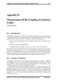
Appendix E – University <strong>of</strong> Hull<br />
E1<br />
Appendix E – <strong>Description</strong> <strong>of</strong> <strong>Measurements</strong> <strong>at</strong> W<strong>at</strong>erloo<br />
<strong>Railway</strong> St<strong>at</strong>ion<br />
In order to verify the computer-based methods used for modelling the ensemble<br />
electromagnetic emissions from a number <strong>of</strong> mobile sources, real measurements, in a<br />
real world environment, were taken. These measurements were carried out in a large,<br />
densly popul<strong>at</strong>ed railway st<strong>at</strong>ion.<br />
E.1 <strong>Measurements</strong> and Equipment<br />
Occupancy monitoring was carried out over a 24 hour period, commencing just after<br />
1500 on 3 December 1997. GSM900 and DCS1800(PCN) mobile channels were<br />
monitored. The following equipment was used:<br />
Rhode and Schwarz HL 024A2 cross log periodic antenna (oper<strong>at</strong>ional from 1 to 18<br />
GHz, used to receive DCS1800)<br />
Emco 3146A log periodic antenna (oper<strong>at</strong>ional from 300MHz to 1GHz, used to<br />
receive GSM900)<br />
WJ 8969 microwave receiver (oper<strong>at</strong>ional from 1 to 18GHz, used to down convert<br />
DCS1800)<br />
Rhode and Schwarz ESMA scanning receiver (oper<strong>at</strong>ional over 20 to 1300MHz -<br />
hence the need to down convert DCS1800)<br />
Interconnecting cables, signal combiner, <strong>at</strong>tenu<strong>at</strong>or and GSM900 bandpass filter (in<br />
order to elimin<strong>at</strong>e signals <strong>at</strong> the down converted frequency).<br />
<strong>Measurements</strong> were performed with IF bandwidths <strong>of</strong> 15, 100 and 2000 kHz with the<br />
number <strong>of</strong> measurements taken <strong>at</strong> each bandwidth in the r<strong>at</strong>io 5:2:1 respectively.<br />
DCS1800(PCN) mobile transmit: 1721.5 to 1781.5 MHz. Channel separ<strong>at</strong>ion:<br />
200kHz.
Appendix E – University <strong>of</strong> Hull<br />
E2<br />
Figure E1: A typical d<strong>at</strong>a file<br />
The column headings represented the following parameters: Frequency / MHz, Start<br />
d<strong>at</strong>e, Start time, Thousandths <strong>of</strong> sec, End d<strong>at</strong>e, End time, Thousandths <strong>of</strong> sec,<br />
Minimum level, Maximum level. This gives us tables <strong>of</strong> the form:<br />
The signal strength units are dBuV, However the system was not calibr<strong>at</strong>ed and level<br />
measurements can only be considered rel<strong>at</strong>ive to each other.<br />
The files for the IF bandwidth <strong>of</strong> 15 kHz contain the 126 slots centred around the<br />
frequencies:<br />
890.0 MHz, 890.2 MHz, 890.4 MHz, ..., 915.0MHz<br />
Note the 200kHz separ<strong>at</strong>ion. The following diagram represents frequency slots<br />
covered by these centre frequencies with a bandwidth <strong>of</strong> 15 kHz<br />
Figure E2: Frequency slots covered by the 15kHz files.<br />
Note, the frequency slot covered by a frequency, with a bandwidth <strong>of</strong> 15 kHz,<br />
represents 0.7% <strong>of</strong> the channel centred <strong>at</strong> th<strong>at</strong> frequency.
Appendix E – University <strong>of</strong> Hull<br />
E3<br />
The files for the IF bandwidth <strong>of</strong> 100 kHz contain the 126 slots centred around the<br />
frequencies:<br />
890.01 MHz, 890.21 MHz, 890.41 MHz, ..., 915.01 MHz<br />
Again we have a 200kHz separ<strong>at</strong>ion between centre frequencies. The frequency slot<br />
covered by a frequency, with a 100 kHz bandwidth, represents 50% <strong>of</strong> the channel<br />
centred <strong>at</strong> these frequencies.<br />
The following diagram represents the frequency slots covered by these centre<br />
frequencies with a bandwidth <strong>of</strong> 100kHz<br />
Figure E3: The frequency slots covered by the 100kHz files.<br />
The files for the IF bandwidth <strong>of</strong> 2 MHz have frequencies centred around<br />
890.02 MHz, 891.02 MHz, 892.02 MHz, ..., 915.02 MHz<br />
Here we have a 1MHz frequency separ<strong>at</strong>ion.<br />
The following diagram represents the frequency slots covered by these centre<br />
frequencies when the bandwidth is 2 MHz N.B. the slots covered by these centre<br />
frequencies overlap. Each slot covers 10 channels.<br />
Figure E4: The frequency slots covered by the 2Mhz files.<br />
If we select a single frequency , say 892 MHz and look <strong>at</strong> the 2MHz bandwidth slot<br />
th<strong>at</strong> it falls into, together with the slots from the 15 and 100 files th<strong>at</strong> also fall into this<br />
slot then we have the following diagram.
E4Appendix E – University <strong>of</strong> Hull<br />
E4<br />
Figure E5: The total frequency slots covered by the recorded d<strong>at</strong>a.<br />
The decision threshold level (which we have taken to be the minimum <strong>of</strong> the minimum<br />
levels recorded for each file) is 7 for the GSM15 files, 15 for the GSM 100 files and 25<br />
for the GSM2 files.<br />
E2. Method for recording minimum and maximum levels<br />
The following explains, by example, the method used for cre<strong>at</strong>ing the excel d<strong>at</strong>a sheets.<br />
FigureE6: A random waveform.<br />
We follow the random signal waveform shown in the above diagram, starting <strong>at</strong> t1.<br />
When the signal rises above the threshold level, i.e. <strong>at</strong> t3, we record start and end<br />
times, the minimum and maximum levels and move on to the next time point. If the<br />
signal level is above the threshold, the minimum and maximum levels are upd<strong>at</strong>ed and<br />
the end time changed to the current time point. This continues until the signal falls<br />
below the threshold again. The final entry in this sequence is the only entry th<strong>at</strong> is<br />
input into the actual d<strong>at</strong>a sheets.
Appendix E – University <strong>of</strong> Hull<br />
E5<br />
Start time End time Minimum level Maximum level<br />
t3 t3 C C<br />
t3 t4 C D<br />
t3 t5 C E<br />
t3 t6 C E<br />
t3 t7 G E<br />
t9 t9 I I<br />
t11 t11 K K<br />
t11 t12 K L<br />
t11 t13 K L<br />
t11 t14 N L<br />
t16 t16 P P<br />
t16 t17 P Q<br />
Table E1: The actual recorded chart only contains the highlighted row, giving the<br />
following d<strong>at</strong>a chart.<br />
Start time End time Minimum level Maximum level<br />
t3 t7 G E<br />
t9 t9 I I<br />
t11 t14 N L<br />
t16 t17 P Q<br />
Notes:<br />
Table E2: Actual recorded excel d<strong>at</strong>a chart.<br />
The actual level may go above the threshold and not get recorded since it falls between<br />
sample times, as, for example, between R and S.<br />
The recorded maximum need not be the true maximum since it may reach a higher<br />
level between sample times, as between P and Q.<br />
If only one sample value lies above the threshold before dropping below it again, as,<br />
for example, <strong>at</strong> I, then the entry in the table will have identical start and end times.<br />
Note where there are only two points above the line, as, for example, <strong>at</strong> P and Q, the<br />
difference between the start and end times recorded in the chart must be the sampling<br />
time.<br />
For each entry in the chart we call the difference between the start time and the end<br />
time the dur<strong>at</strong>ion. The minimum dur<strong>at</strong>ion recorded for the GSM15 files is 2.8 secs, for<br />
the GSM 100 files it is 8.8 secs and for the GSM2 files, it is 19.8 secs.
Appendix E – University <strong>of</strong> Hull<br />
E6<br />
Filename Length <strong>of</strong> time covered Min dur<strong>at</strong>ion min (min) max (max)<br />
gsm2a 01:57:51 19.7769 25 64<br />
gsm2b 01:33:22 19.7783 25 64<br />
gsm2c 01:36:39 19.7792 25 62<br />
gsm2d 01:57:10 19.7721 25 61<br />
gsm2e 10:33:11 19.8128 25 66<br />
gsm2f 02:41:01 19.7795 25 83<br />
gsm2g 02:39:40 19.8014 25 75<br />
gsm2h 02:04:12 19.7784 25 73<br />
gsm100a 01:57:52 8.7986 15 67<br />
gsm100b 01:33:53 8.7983 15 67<br />
gsm100c 01:36:40 8.7986 15 67<br />
gsm100d 01:57:20 8.7983 15 66<br />
gsm100e 10:33:20 8.8127 15 65<br />
gsm100f 02:41:01 8.8108 15 83<br />
gsm100g 02:40:00 8.8128 15 83<br />
gsm100h 02:04:21 8.8 15 75<br />
gsm15a 01:58:00 2.7732 7 64<br />
gsm15b 01:33:48 2.7734 7 64<br />
gsm15c 01:36:54 2.773 7 64<br />
gsm15d 01:57:15 2.7723 7 60<br />
gsm15e 10:33:32 2.7726 7 58<br />
gsm15f 02:41:09 2.7726 7 83<br />
gsm15g 02:40:00 2.774 7 83<br />
gsm15h 02:04:32 2.7737 7 77<br />
Table E3:<br />
Summary chart <strong>of</strong> the gsm files.<br />
If we take another look <strong>at</strong> Table E1 all we are actually given in this situ<strong>at</strong>ion is Table<br />
E2 and all th<strong>at</strong> we can determine from this table is represented by the following<br />
diagram:<br />
Figure E7: Graphical represent<strong>at</strong>ion <strong>of</strong> Table E2.
Appendix E – University <strong>of</strong> Hull<br />
E7<br />
We only know the recorded minimum and maximum levels. We cannot say anything<br />
about wh<strong>at</strong> goes on in-between time samples.<br />
N.B. This is for a single frequency only, each file contains 126 different frequencies.<br />
To look <strong>at</strong> a single frequency as above, we have to go through each file and extract the<br />
relevant lines. For example, if we take the frequency 890.41MHz with an IF<br />
bandwidth <strong>of</strong> 100kHz, we have to extract the relevant parts <strong>of</strong> the files GSM100a-<br />
GSM100h, i.e. the lines with 890.41 in the first column. These 8 parts (one from each<br />
<strong>of</strong> the 8 files) are put into a single d<strong>at</strong>a sheet. We have also calcul<strong>at</strong>ed the minimum<br />
and maximum <strong>of</strong> the minimum and maximum levels and added these to the chart. This<br />
gives the following chart:<br />
N.B. This is one <strong>of</strong> the smaller files, when some channels are extracted the resulting<br />
chart can be as many as a few thousand line long. This method is therefore very time<br />
consuming.<br />
We have converted the start/end d<strong>at</strong>e and times into times after 00:00:00 on 03/12/97.<br />
With this definition <strong>of</strong> the start and end times we are able to calcul<strong>at</strong>e the dur<strong>at</strong>ion for<br />
each entry and then the midpoint between the start and end time - we call this the<br />
“middle”.<br />
Note, the majority <strong>of</strong> the entries have identical start and end times, this indic<strong>at</strong>es th<strong>at</strong><br />
only a single sample lies above the threshold.<br />
If we plot the minimum and maximum levels against the “middle” value then we get<br />
the following graph:<br />
40<br />
35<br />
Minimum and maximum levels.<br />
30<br />
25<br />
Min level<br />
Max level<br />
20<br />
15<br />
55671.94<br />
58106.41<br />
61769.85<br />
62465.16<br />
63299.49<br />
63846.46<br />
65761.91<br />
66278.73<br />
66488.41<br />
67113.12<br />
68205.95<br />
68634.3<br />
69254.21<br />
69655.83<br />
72426.71<br />
73816.79<br />
75076.7<br />
76001.22<br />
77351.49<br />
79496.87<br />
31863.18<br />
36091.09<br />
43937.32<br />
46142.61<br />
54032.89<br />
55434.95<br />
Time after 00:00:00 on 03/12/97 in seconds.<br />
Figure E8: Minimum and maximum levels for the centre frequency 890.41MHz with<br />
100kHz bandwidth.
Appendix E – University <strong>of</strong> Hull<br />
E8<br />
Taking individual channels we formed a probability distribution function for the<br />
minimum and maximum levels. We did this for the three different bandwidths <strong>of</strong><br />
15kHz, 100kHz and 2kHz. Examples <strong>of</strong> these level distributions are shown below.<br />
percentage<br />
Min and max level distribution for centre frequency 890.40MHz (GSM) with 15kHz bandwidth<br />
35<br />
30<br />
25<br />
20<br />
15<br />
Minimum level<br />
Maximum level<br />
10<br />
5<br />
0<br />
0 3 6 9 12 15 18 21 24 27 30 33 36 39 42 45 48 51 54 57 60 63 66 69 72 75 78 81 84 87 90 93 96 99<br />
Rel<strong>at</strong>ive level dB<br />
percentage<br />
35<br />
Min and max level distribution for centre frequency 890.60MHz (GSM) with 15kHz bandwidth<br />
30<br />
25<br />
20<br />
15<br />
Minimum level<br />
Maximum level<br />
10<br />
5<br />
0<br />
0 3 6 9 12 15 18 21 24 27 30 33 36 39 42 45 48 51 54 57 60 63 66 69 72 75 78 81 84 87 90 93 96 99<br />
Rel<strong>at</strong>ive level dB<br />
percentage<br />
Min and max level distribution for centre frequency 890.80MHz (GSM) with 15kHz bandwidth<br />
35<br />
30<br />
25<br />
20<br />
15<br />
Minimum level<br />
Maximum level<br />
10<br />
5<br />
0<br />
0 3 6 9 12 15 18 21 24 27 30 33 36 39 42 45 48 51 54 57 60 63 66 69 72 75 78 81 84 87 90 93 96 99<br />
Rel<strong>at</strong>ive level dB<br />
Figure E9: Examples <strong>of</strong> level distributions for channels with a 15kHz bandwidth.
Appendix E – University <strong>of</strong> Hull<br />
E9<br />
percentage<br />
35<br />
Min and max level distribution for centre frequency 890.41MHz (GSM) with 100kHz bandwidth<br />
30<br />
25<br />
20<br />
15<br />
Minimum level<br />
Maximum level<br />
10<br />
5<br />
0<br />
0 3 6 9 12 15 18 21 24 27 30 33 36 39 42 45 48 51 54 57 60 63 66 69 72 75 78 81 84 87 90 93 96 99<br />
Rel<strong>at</strong>ive level dB<br />
percentage<br />
35<br />
Min and max level distribution for centre frequency 890.61MHz (GSM) with 100kHz bandwidth<br />
30<br />
25<br />
20<br />
15<br />
Minimum level<br />
Maximum level<br />
10<br />
5<br />
0<br />
0 3 6 9 12 15 18 21 24 27 30 33 36 39 42 45 48 51 54 57 60 63 66 69 72 75 78 81 84 87 90 93 96 99<br />
Rel<strong>at</strong>ive level dB<br />
percentage<br />
Min and max level distribution for centre frequency 890.81MHz (GSM) with 100kHz bandwidth<br />
35<br />
30<br />
25<br />
20<br />
15<br />
Minimum level<br />
Maximum level<br />
10<br />
5<br />
0<br />
0 3 6 9 12 15 18 21 24 27 30 33 36 39 42 45 48 51 54 57 60 63 66 69 72 75 78 81 84 87 90 93 96 99<br />
Rel<strong>at</strong>ive level dB<br />
Figure E10: Examples <strong>of</strong> level distributions for channels with a 100kHz bandwidth.
Appendix E – University <strong>of</strong> Hull<br />
E10<br />
percentage<br />
35<br />
Min and max level distribution for centre frequency 892.02MHz (GSM) with 2MHz bandwidth<br />
30<br />
25<br />
20<br />
15<br />
Minimum level<br />
Maximum level<br />
10<br />
5<br />
0<br />
0 3 6 9 12 15 18 21 24 27 30 33 36 39 42 45 48 51 54 57 60 63 66 69 72 75 78 81 84 87 90 93 96 99<br />
Rel<strong>at</strong>ive level dB<br />
percentage<br />
35<br />
Min and max level distribution for centre frequency 893.02MHz (GSM) with 2MHz bandwidth<br />
30<br />
25<br />
20<br />
15<br />
Minimum level<br />
Maximum level<br />
10<br />
5<br />
0<br />
0 3 6 9 12 15 18 21 24 27 30 33 36 39 42 45 48 51 54 57 60 63 66 69 72 75 78 81 84 87 90 93 96 99<br />
Rel<strong>at</strong>ive level dB<br />
percentage<br />
35<br />
Min and max level distribution for centre frequency 894.02MHz (GSM) with 2MHz bandwidth<br />
30<br />
25<br />
20<br />
15<br />
Minimum level<br />
Maximum level<br />
10<br />
5<br />
0<br />
0 3 6 9 12 15 18 21 24 27 30 33 36 39 42 45 48 51 54 57 60 63 66 69 72 75 78 81 84 87 90 93 96 99<br />
Rel<strong>at</strong>ive level dB<br />
Figure E1.: Examples <strong>of</strong> level distributions for channels with a 2MHz bandwidth.
Appendix E – University <strong>of</strong> Hull<br />
E11<br />
We then took the average distribution for each <strong>of</strong> the three bandwidths.<br />
percentage<br />
20<br />
Average distribution taken from the 15 files<br />
18<br />
16<br />
14<br />
12<br />
10<br />
min<br />
max<br />
8<br />
6<br />
4<br />
2<br />
0<br />
0 3 6 9 12 15 18 21 24 27 30 33 36 39 42 45 48 51 54 57 60 63 66 69 72 75 78 81 84 87 90 93 96 99<br />
Rel<strong>at</strong>ive level dB<br />
percentage<br />
20<br />
Average distribution taken over all the 100 files<br />
18<br />
16<br />
14<br />
12<br />
10<br />
min<br />
max<br />
8<br />
6<br />
4<br />
2<br />
0<br />
0 3 6 9 12 15 18 21 24 27 30 33 36 39 42 45 48 51 54 57 60 63 66 69 72 75 78 81 84 87 90 93 96 99<br />
Rel<strong>at</strong>ive level dB<br />
percentage<br />
20<br />
Average distribution taken from all the "GSM2 files".<br />
18<br />
16<br />
14<br />
12<br />
10<br />
min<br />
max<br />
8<br />
6<br />
4<br />
2<br />
0<br />
0 3 6 9 12 15 18 21 24 27 30 33 36 39 42 45 48 51 54 57 60 63 66 69 72 75 78 81 84 87 90 93 96 99<br />
Rel<strong>at</strong>ive level dB<br />
Figure E12: The average distributions for the three different bandwidths.
Appendix E – University <strong>of</strong> Hull<br />
E12<br />
percentage<br />
20<br />
Average distribution for the gsm2 files after spreading the initial spike over the below threshold values.<br />
18<br />
16<br />
14<br />
12<br />
10<br />
min<br />
max<br />
8<br />
6<br />
4<br />
2<br />
0<br />
0 3 6 9 12 15 18 21 24 27 30 33 36 39 42 45 48 51 54 57 60 63 66 69 72 75 78 81 84 87 90 93 96 99<br />
Rel<strong>at</strong>ive level dB<br />
percentage<br />
20<br />
Average distribution for the gsm100 filesafter spreading the initial spike over the below threshold values.<br />
18<br />
16<br />
14<br />
12<br />
10<br />
min<br />
max<br />
8<br />
6<br />
4<br />
2<br />
0<br />
0 3 6 9 12 15 18 21 24 27 30 33 36 39 42 45 48 51 54 57 60 63 66 69 72 75 78 81 84 87 90 93 96 99<br />
Rel<strong>at</strong>ive level dB<br />
percentage<br />
20<br />
Average distribution for the gsm15 files after spreading the initial spike over the below threshold values.<br />
18<br />
16<br />
14<br />
12<br />
10<br />
min<br />
max<br />
8<br />
6<br />
4<br />
2<br />
0<br />
0 3 6 9 12 15 18 21 24 27 30 33 36 39 42 45 48 51 54 57 60 63 66 69 72 75 78 81 84 87 90 93 96 99<br />
Rel<strong>at</strong>ive level dB<br />
Figure E13: Average distributions for each bandwidth , with the initial spike spread<br />
over the below threshold levels.