SPECT reconstruction
SPECT reconstruction
SPECT reconstruction

You also want an ePaper? Increase the reach of your titles
YUMPU automatically turns print PDFs into web optimized ePapers that Google loves.
Regional Training Workshop<br />
Advanced Image Processing of <strong>SPECT</strong> Studies<br />
Tygerberg Hospital, 19-23 April 2004<br />
<strong>SPECT</strong> <strong>reconstruction</strong><br />
Martin Šámal<br />
Charles University Prague, Czech Republic<br />
samal@cesnet.cz
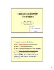
Tomography is performed in 2 steps:<br />
1st step = data acquisition (record of projections)<br />
The result is a set of angular projections.<br />
The set of projections of a single slice is called sinogram.<br />
2nd step = image recontruction from projections<br />
There are 2 groups of <strong>reconstruction</strong> methods:<br />
analytic (e.g. FBP = filtered back projection) and<br />
iterative (e.g. ART = algebraic <strong>reconstruction</strong><br />
techniques).
anterior view<br />
lateral view<br />
courtesy of Dr. K. Kouris
1st step in tomography = recording projections<br />
courtesy of Dr. K. Kouris
Groch MW, Erwin WD. J Nucl Med Technol 2000;28:233-244.
Sinogram = collection of projections of a single slice
2nd step in tomography = <strong>reconstruction</strong><br />
from projections<br />
Analytic <strong>reconstruction</strong> methods (e.g. the filtered backprojection<br />
algorithm) are efficient (fast) and elegant, but<br />
they are unable to handle complicated factors such as<br />
scatter. Filtered back projection has been used for<br />
<strong>reconstruction</strong>s in x-ray CT and for most <strong>SPECT</strong> and PET<br />
<strong>reconstruction</strong>s until recently.<br />
Iterative <strong>reconstruction</strong> algorithms, on the other hand,<br />
are more versatile but less efficient. Efficient (that is - fast)<br />
iterative algorithms are currently under development. With<br />
rapid increases being made in computer speed and<br />
memory, iterative <strong>reconstruction</strong> algorithms will be used in<br />
more and more applications of <strong>SPECT</strong> and PET and will<br />
enable more quantitative <strong>reconstruction</strong>s.
Analytic <strong>reconstruction</strong> methods<br />
(projection - backprojection algorithms)<br />
filtered back-projection<br />
back-projection filtering<br />
Radon J.<br />
On the determination of functions from their integrals along<br />
certain manifolds [in German].<br />
Math Phys Klass 1917;69:262-277.
Recording projections of a slice
Back projection (BP)
Filtered back-projection (FBP)
1 2<br />
3 4
1 2<br />
3 4
1 2<br />
3 4
1 2<br />
3<br />
3 4<br />
7<br />
1<br />
5<br />
4<br />
2<br />
5<br />
4 6<br />
3
0 0<br />
3<br />
0 0<br />
7<br />
1<br />
5<br />
4<br />
2<br />
5<br />
4 6<br />
3
3 3<br />
3<br />
7 7<br />
7<br />
1<br />
5<br />
4<br />
2<br />
5<br />
4 6<br />
3
8 5<br />
3<br />
10 12<br />
7<br />
1<br />
5<br />
4<br />
2<br />
5<br />
4 6<br />
3
12 11<br />
3<br />
14 18<br />
7<br />
1<br />
5<br />
4<br />
2<br />
5<br />
4 6<br />
3
- 10 (subtract total sum from each entry)<br />
13 16<br />
3<br />
19 22<br />
7<br />
1<br />
5<br />
4<br />
2<br />
5<br />
4 6<br />
3
3 (divide each entry by 3)<br />
3 6<br />
4<br />
9 12<br />
7<br />
1<br />
5<br />
4<br />
2<br />
5<br />
4 6<br />
3
1 2<br />
4<br />
3 4<br />
7<br />
1<br />
5<br />
4<br />
2<br />
5<br />
4 6<br />
3
ack projection (BP) = summation of projections
filtered back projection (FBP)
Sequence of summing original and filtered projections<br />
back projection<br />
filtered back projection
Reconstruction of a slice from projections<br />
example = myocardial perfusion, left ventricle, long axis<br />
y<br />
Count rate<br />
y<br />
z<br />
x<br />
x-position<br />
z<br />
courtesy of Dr. K. Kouris
Reconstruction of a slice from projections<br />
example = myocardial perfusion, left ventricle, long axis<br />
courtesy of Dr. K. Kouris
Iterative <strong>reconstruction</strong> methods<br />
conventional iterative algebraic methods<br />
algebraic <strong>reconstruction</strong> technique (ART)<br />
simultaneous iterative <strong>reconstruction</strong> technique (SIRT)<br />
iterative least-squares technique (ILST)<br />
iterative statistical <strong>reconstruction</strong> methods<br />
(with and without using a priori information)<br />
gradient and conjugate gradient (CG) algorithms<br />
maximum likelihood expectation maximization (MLEM)<br />
ordered-subsets expectation maximization (OSEM)<br />
maximum a posteriori (MAP) algorithms
The principle of the iterative algorithms is to find a solution<br />
(that is - to reconstruct an image of a tomographic slice from<br />
projections) by successive estimates. The projections<br />
corresponding to the current estimate are compared with the<br />
measured projections. The result of the comparison is used to<br />
modify the current estimate, thereby creating a new estimate.<br />
The algorithms differ in the way the measured and estimated<br />
projections are compared and the kind of correction applied to<br />
the current estimate. The process is initiated by arbitrarily<br />
creating a first estimate - for example, a uniform image (all<br />
pixels equal zero, one, or a mean pixel value,…). Corrections<br />
are carried out either as addition of differences or multiplication<br />
by quotients between measured and estimated projections.
algorithm (a recipe)<br />
(1) make the first arbitrary estimate of the slice (homogeneous image),<br />
(2) project the estimated slice into projections analogous to those<br />
measured by the camera (important: in this step, physical corrections<br />
can be introduced - for attenuation, scatter, and depth-dependent<br />
collimator resolution),<br />
(3) compare the projections of the estimate with measured projections<br />
(subtract or divide the corresponding projections in order to obtain<br />
correction factors - in the form of differences or quotients),<br />
(4) stop or continue: if the correction factors are approaching zero, if<br />
they do not change in subsequent iterations, or if the maximum number<br />
of iterations was achieved, then finish; otherwise<br />
(5) apply corrections to the estimate (add the differences to individual<br />
pixels or multiply pixel values by correction quotients) - thus make the<br />
new estimate of the slice,<br />
(6) go to step (2).
measured<br />
projections<br />
first estimate<br />
and its<br />
projections<br />
correction<br />
factors<br />
(differences<br />
between<br />
projections)<br />
measured<br />
projections<br />
first estimate<br />
and its<br />
projections<br />
correction<br />
factors<br />
(quotients<br />
between<br />
projections)
first<br />
iteration<br />
(additive<br />
corrections)<br />
second<br />
iteration<br />
(additive<br />
corrections)<br />
first<br />
iteration<br />
(multiplicat.<br />
corrections)<br />
second<br />
iteration<br />
(multiplicat.<br />
corrections)
1 2<br />
3<br />
2.5 2.5<br />
5<br />
3 4<br />
7<br />
2.5 2.5<br />
5<br />
4 6<br />
5 5<br />
c11 = (3 - 5)/2 + (4 - 5)/2 = -2/2 - 1/2<br />
c11 = -1 - 0.5 = -1.5
1 2<br />
3<br />
2.5 2.5<br />
5<br />
3 4<br />
7<br />
2.5 2.5<br />
5<br />
4 6<br />
5 5<br />
c11 = (3 - 5)/2 + (4 - 5)/2 = -2/2 - 1/2<br />
c11 = -1 - 0.5 = -1.5
1 2<br />
3<br />
1 2.5<br />
5<br />
3 4<br />
7<br />
2.5 2.5<br />
5<br />
4 6<br />
5 5<br />
c12 = (3 - 5)/2 + (6 - 5)/2 = -2/2 + 1/2<br />
c12 = -1 + 0.5 = -0.5
1 2<br />
3<br />
1 2<br />
5<br />
3 4<br />
7<br />
2.5 2.5<br />
5<br />
4 6<br />
5 5<br />
c13 = (7 - 5)/2 + (4 - 5)/2 = 2/2 - 1/2<br />
c13 = 1 - 0.5 = 0.5
1 2<br />
3<br />
1 2<br />
5<br />
3 4<br />
7<br />
3 2.5<br />
5<br />
4 6<br />
5 5<br />
c14 = (7 - 5)/2 + (6 - 5)/2 = 2/2 + 1/2<br />
c14 = 1 + 0.5 = 1.5
1 2<br />
3<br />
1 2<br />
5<br />
3 4<br />
7<br />
3 4<br />
5<br />
4 6<br />
5 5
Iterative <strong>reconstruction</strong> - multiplicative corrections
Iterative <strong>reconstruction</strong> - differences between individual<br />
iterations
Iterative <strong>reconstruction</strong> - multiplicative corrections
Sequence of iterations - multiplicative corrections<br />
estimated image<br />
differences between<br />
subsequent iterations
Filtered back-projection<br />
• very fast<br />
• direct inversion of the<br />
projection formula<br />
• corrections for scatter,<br />
non-uniform attenuation<br />
and other physical factors<br />
are difficult<br />
• it needs a lot of filtering -<br />
trade-off between blurring<br />
and noise<br />
• quantitative imaging<br />
difficult
Iterative <strong>reconstruction</strong><br />
• discreteness of data<br />
included in the model<br />
• it is easy to model and<br />
handle projection noise,<br />
especially when the<br />
counts are low<br />
• it is easy to model the<br />
imaging physics such as<br />
geometry, non-uniform<br />
attenuation, scatter, etc.<br />
• quantitative imaging<br />
possible<br />
• amplification of noise<br />
• long calculation time
References:<br />
Groch MW, Erwin WD. <strong>SPECT</strong> in the year 2000: basic principles.<br />
J Nucl Med Techol 2000; 28:233-244, http://www.snm.org.<br />
Groch MW, Erwin WD. Single-photon emission computed tomography<br />
in the year 2001: instrumentation and quality control.<br />
J Nucl Med Technol 2001; 20:9-15, http://www.snm.org.<br />
Bruyant PP. Analytic and iterative <strong>reconstruction</strong> algorithms in <strong>SPECT</strong>.<br />
J Nucl Med 2002; 43:1343-1358, http://www.snm.org.<br />
Zeng GL. Image <strong>reconstruction</strong> - a tutorial.<br />
Computerized Med Imaging and Graphics 2001; 25(2):97-103,<br />
http://www.elsevier.com/locate/compmedimag.<br />
Vandenberghe S et al. Iterative <strong>reconstruction</strong> algorithms in nuclear<br />
medicine. Computerized Med Imaging and Graphics 2001; 25(2):105-111,<br />
http://www.elsevier.com/locate/compmedimag.
References:<br />
Patterson HE, Hutton BF (eds.). Distance Assisted Training Programme<br />
for Nuclear Medicine Technologists. IAEA, Vienna, 2003,<br />
http://www.iaea.org.<br />
Busemann-Sokole E. IAEA Quality Control Atlas for Scintillation Camera<br />
Systems. IAEA, Vienna, 2003, ISBN 92-0-101303-5,<br />
http://www.iaea.org/worldatom/books, http://www.iaea.org/Publications.<br />
Steves AM. Review of nuclear medicine technology. Society of Nuclear<br />
Medicine Inc., Reston, 1996, ISBN 0-032004-45-8, http://www.snm.org.<br />
Steves AM. Preparation for examinations in nuclear medicine<br />
technology. Society of Nuclear Medicine Inc., Reston, 1997,<br />
ISBN 0-932004-49-0, http://www.snm.org.<br />
Graham LS (ed.). Nuclear medicine self study program II:<br />
Instrumentation. Society of Nuclear Medicine Inc., Reston, 1996,<br />
ISBN 0-932004-44-X, http://www.snm.org.<br />
Saha GB. Physics and radiobiology of nuclear medicine. Springer-<br />
Verlag, New York, 1993, ISBN 3-540-94036-7.