SPECT reconstruction
SPECT reconstruction
SPECT reconstruction

Create successful ePaper yourself
Turn your PDF publications into a flip-book with our unique Google optimized e-Paper software.
Regional Training Workshop<br />
Advanced Image Processing of <strong>SPECT</strong> Studies<br />
Tygerberg Hospital, 19-23 April 2004<br />
<strong>SPECT</strong> <strong>reconstruction</strong><br />
Martin Šámal<br />
Charles University Prague, Czech Republic<br />
samal@cesnet.cz
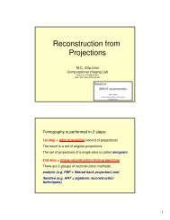
Tomography is performed in 2 steps:<br />
1st step = data acquisition (record of projections)<br />
The result is a set of angular projections.<br />
The set of projections of a single slice is called sinogram.<br />
2nd step = image recontruction from projections<br />
There are 2 groups of <strong>reconstruction</strong> methods:<br />
analytic (e.g. FBP = filtered back projection) and<br />
iterative (e.g. ART = algebraic <strong>reconstruction</strong><br />
techniques).
anterior view<br />
lateral view<br />
courtesy of Dr. K. Kouris
1st step in tomography = recording projections<br />
courtesy of Dr. K. Kouris
Groch MW, Erwin WD. J Nucl Med Technol 2000;28:233-244.
Sinogram = collection of projections of a single slice
2nd step in tomography = <strong>reconstruction</strong><br />
from projections<br />
Analytic <strong>reconstruction</strong> methods (e.g. the filtered backprojection<br />
algorithm) are efficient (fast) and elegant, but<br />
they are unable to handle complicated factors such as<br />
scatter. Filtered back projection has been used for<br />
<strong>reconstruction</strong>s in x-ray CT and for most <strong>SPECT</strong> and PET<br />
<strong>reconstruction</strong>s until recently.<br />
Iterative <strong>reconstruction</strong> algorithms, on the other hand,<br />
are more versatile but less efficient. Efficient (that is - fast)<br />
iterative algorithms are currently under development. With<br />
rapid increases being made in computer speed and<br />
memory, iterative <strong>reconstruction</strong> algorithms will be used in<br />
more and more applications of <strong>SPECT</strong> and PET and will<br />
enable more quantitative <strong>reconstruction</strong>s.
Analytic <strong>reconstruction</strong> methods<br />
(projection - backprojection algorithms)<br />
filtered back-projection<br />
back-projection filtering<br />
Radon J.<br />
On the determination of functions from their integrals along<br />
certain manifolds [in German].<br />
Math Phys Klass 1917;69:262-277.
Recording projections of a slice
Back projection (BP)
Filtered back-projection (FBP)
1 2<br />
3 4
1 2<br />
3 4
1 2<br />
3 4
1 2<br />
3<br />
3 4<br />
7<br />
1<br />
5<br />
4<br />
2<br />
5<br />
4 6<br />
3
0 0<br />
3<br />
0 0<br />
7<br />
1<br />
5<br />
4<br />
2<br />
5<br />
4 6<br />
3
3 3<br />
3<br />
7 7<br />
7<br />
1<br />
5<br />
4<br />
2<br />
5<br />
4 6<br />
3
8 5<br />
3<br />
10 12<br />
7<br />
1<br />
5<br />
4<br />
2<br />
5<br />
4 6<br />
3
12 11<br />
3<br />
14 18<br />
7<br />
1<br />
5<br />
4<br />
2<br />
5<br />
4 6<br />
3
- 10 (subtract total sum from each entry)<br />
13 16<br />
3<br />
19 22<br />
7<br />
1<br />
5<br />
4<br />
2<br />
5<br />
4 6<br />
3
3 (divide each entry by 3)<br />
3 6<br />
4<br />
9 12<br />
7<br />
1<br />
5<br />
4<br />
2<br />
5<br />
4 6<br />
3
1 2<br />
4<br />
3 4<br />
7<br />
1<br />
5<br />
4<br />
2<br />
5<br />
4 6<br />
3
ack projection (BP) = summation of projections
filtered back projection (FBP)
Sequence of summing original and filtered projections<br />
back projection<br />
filtered back projection
Reconstruction of a slice from projections<br />
example = myocardial perfusion, left ventricle, long axis<br />
y<br />
Count rate<br />
y<br />
z<br />
x<br />
x-position<br />
z<br />
courtesy of Dr. K. Kouris
Reconstruction of a slice from projections<br />
example = myocardial perfusion, left ventricle, long axis<br />
courtesy of Dr. K. Kouris
Iterative <strong>reconstruction</strong> methods<br />
conventional iterative algebraic methods<br />
algebraic <strong>reconstruction</strong> technique (ART)<br />
simultaneous iterative <strong>reconstruction</strong> technique (SIRT)<br />
iterative least-squares technique (ILST)<br />
iterative statistical <strong>reconstruction</strong> methods<br />
(with and without using a priori information)<br />
gradient and conjugate gradient (CG) algorithms<br />
maximum likelihood expectation maximization (MLEM)<br />
ordered-subsets expectation maximization (OSEM)<br />
maximum a posteriori (MAP) algorithms
The principle of the iterative algorithms is to find a solution<br />
(that is - to reconstruct an image of a tomographic slice from<br />
projections) by successive estimates. The projections<br />
corresponding to the current estimate are compared with the<br />
measured projections. The result of the comparison is used to<br />
modify the current estimate, thereby creating a new estimate.<br />
The algorithms differ in the way the measured and estimated<br />
projections are compared and the kind of correction applied to<br />
the current estimate. The process is initiated by arbitrarily<br />
creating a first estimate - for example, a uniform image (all<br />
pixels equal zero, one, or a mean pixel value,…). Corrections<br />
are carried out either as addition of differences or multiplication<br />
by quotients between measured and estimated projections.
algorithm (a recipe)<br />
(1) make the first arbitrary estimate of the slice (homogeneous image),<br />
(2) project the estimated slice into projections analogous to those<br />
measured by the camera (important: in this step, physical corrections<br />
can be introduced - for attenuation, scatter, and depth-dependent<br />
collimator resolution),<br />
(3) compare the projections of the estimate with measured projections<br />
(subtract or divide the corresponding projections in order to obtain<br />
correction factors - in the form of differences or quotients),<br />
(4) stop or continue: if the correction factors are approaching zero, if<br />
they do not change in subsequent iterations, or if the maximum number<br />
of iterations was achieved, then finish; otherwise<br />
(5) apply corrections to the estimate (add the differences to individual<br />
pixels or multiply pixel values by correction quotients) - thus make the<br />
new estimate of the slice,<br />
(6) go to step (2).
measured<br />
projections<br />
first estimate<br />
and its<br />
projections<br />
correction<br />
factors<br />
(differences<br />
between<br />
projections)<br />
measured<br />
projections<br />
first estimate<br />
and its<br />
projections<br />
correction<br />
factors<br />
(quotients<br />
between<br />
projections)
first<br />
iteration<br />
(additive<br />
corrections)<br />
second<br />
iteration<br />
(additive<br />
corrections)<br />
first<br />
iteration<br />
(multiplicat.<br />
corrections)<br />
second<br />
iteration<br />
(multiplicat.<br />
corrections)
1 2<br />
3<br />
2.5 2.5<br />
5<br />
3 4<br />
7<br />
2.5 2.5<br />
5<br />
4 6<br />
5 5<br />
c11 = (3 - 5)/2 + (4 - 5)/2 = -2/2 - 1/2<br />
c11 = -1 - 0.5 = -1.5
1 2<br />
3<br />
2.5 2.5<br />
5<br />
3 4<br />
7<br />
2.5 2.5<br />
5<br />
4 6<br />
5 5<br />
c11 = (3 - 5)/2 + (4 - 5)/2 = -2/2 - 1/2<br />
c11 = -1 - 0.5 = -1.5
1 2<br />
3<br />
1 2.5<br />
5<br />
3 4<br />
7<br />
2.5 2.5<br />
5<br />
4 6<br />
5 5<br />
c12 = (3 - 5)/2 + (6 - 5)/2 = -2/2 + 1/2<br />
c12 = -1 + 0.5 = -0.5
1 2<br />
3<br />
1 2<br />
5<br />
3 4<br />
7<br />
2.5 2.5<br />
5<br />
4 6<br />
5 5<br />
c13 = (7 - 5)/2 + (4 - 5)/2 = 2/2 - 1/2<br />
c13 = 1 - 0.5 = 0.5
1 2<br />
3<br />
1 2<br />
5<br />
3 4<br />
7<br />
3 2.5<br />
5<br />
4 6<br />
5 5<br />
c14 = (7 - 5)/2 + (6 - 5)/2 = 2/2 + 1/2<br />
c14 = 1 + 0.5 = 1.5
1 2<br />
3<br />
1 2<br />
5<br />
3 4<br />
7<br />
3 4<br />
5<br />
4 6<br />
5 5
Iterative <strong>reconstruction</strong> - multiplicative corrections
Iterative <strong>reconstruction</strong> - differences between individual<br />
iterations
Iterative <strong>reconstruction</strong> - multiplicative corrections
Sequence of iterations - multiplicative corrections<br />
estimated image<br />
differences between<br />
subsequent iterations
Filtered back-projection<br />
• very fast<br />
• direct inversion of the<br />
projection formula<br />
• corrections for scatter,<br />
non-uniform attenuation<br />
and other physical factors<br />
are difficult<br />
• it needs a lot of filtering -<br />
trade-off between blurring<br />
and noise<br />
• quantitative imaging<br />
difficult
Iterative <strong>reconstruction</strong><br />
• discreteness of data<br />
included in the model<br />
• it is easy to model and<br />
handle projection noise,<br />
especially when the<br />
counts are low<br />
• it is easy to model the<br />
imaging physics such as<br />
geometry, non-uniform<br />
attenuation, scatter, etc.<br />
• quantitative imaging<br />
possible<br />
• amplification of noise<br />
• long calculation time
References:<br />
Groch MW, Erwin WD. <strong>SPECT</strong> in the year 2000: basic principles.<br />
J Nucl Med Techol 2000; 28:233-244, http://www.snm.org.<br />
Groch MW, Erwin WD. Single-photon emission computed tomography<br />
in the year 2001: instrumentation and quality control.<br />
J Nucl Med Technol 2001; 20:9-15, http://www.snm.org.<br />
Bruyant PP. Analytic and iterative <strong>reconstruction</strong> algorithms in <strong>SPECT</strong>.<br />
J Nucl Med 2002; 43:1343-1358, http://www.snm.org.<br />
Zeng GL. Image <strong>reconstruction</strong> - a tutorial.<br />
Computerized Med Imaging and Graphics 2001; 25(2):97-103,<br />
http://www.elsevier.com/locate/compmedimag.<br />
Vandenberghe S et al. Iterative <strong>reconstruction</strong> algorithms in nuclear<br />
medicine. Computerized Med Imaging and Graphics 2001; 25(2):105-111,<br />
http://www.elsevier.com/locate/compmedimag.
References:<br />
Patterson HE, Hutton BF (eds.). Distance Assisted Training Programme<br />
for Nuclear Medicine Technologists. IAEA, Vienna, 2003,<br />
http://www.iaea.org.<br />
Busemann-Sokole E. IAEA Quality Control Atlas for Scintillation Camera<br />
Systems. IAEA, Vienna, 2003, ISBN 92-0-101303-5,<br />
http://www.iaea.org/worldatom/books, http://www.iaea.org/Publications.<br />
Steves AM. Review of nuclear medicine technology. Society of Nuclear<br />
Medicine Inc., Reston, 1996, ISBN 0-032004-45-8, http://www.snm.org.<br />
Steves AM. Preparation for examinations in nuclear medicine<br />
technology. Society of Nuclear Medicine Inc., Reston, 1997,<br />
ISBN 0-932004-49-0, http://www.snm.org.<br />
Graham LS (ed.). Nuclear medicine self study program II:<br />
Instrumentation. Society of Nuclear Medicine Inc., Reston, 1996,<br />
ISBN 0-932004-44-X, http://www.snm.org.<br />
Saha GB. Physics and radiobiology of nuclear medicine. Springer-<br />
Verlag, New York, 1993, ISBN 3-540-94036-7.