059 - MIT Haystack Observatory

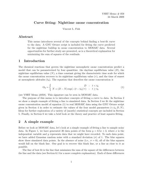
Curve fitting: Nighttime ozone concentration
Vincent L. Fish
VSRT Memo # 059
24 March 2009
Abstract
This memo introduces several of the concepts behind finding a best-fit curve
to the data. A GNU Octave script is included for fitting the curve predicted
for the nighttime buildup in ozone concentration to MOSAIC data. Several
opportunities for further study are presented, as is a theoretical explanation for
minimizing the sum of squares of the residuals.
1 Introduction
The chemical reactions that govern the nighttime mesospheric ozone concentration predict a
model that can be parameterized by four quantities: the daytime equilibrium value (D), the
nighttime equilibrium value (N), a time constant giving the characteristic time scale for which
the ozone concentration recovers to its nighttime equilibrium value (τ), and the time of sunset
at mesospheric altitudes (t 0 ). The equation that describes the ozone concentration is
O 3 =
{
D : t < t 0
N + (D − N)exp(−(t − t 0 )/τ) : t ≥ t 0
(1)
(see VSRT Memo #058). This signature can be seen in MOSAIC data.
The purpose of this memo is to introduce concepts of fitting a curve to data. In Section 2
we show a simple example of fitting a line to simulated data. In Section 3 we fit the nighttime
ozone concentration model of equation (1) to real MOSAIC data using the GNU Octave script
given in Section 4 in order to estimate the values of the four model parameters (τ,t 0 ,D,N).
Ideas for further exploration of a variety of (mostly) statistical concepts are included in Section
5. Finally, in Section 6 we take a brief look at the theory and practice of least squares fitting.
2 A simple example
Before we look at MOSAIC data, let’s look at a simple example of fitting a line to sample noisy
data. In Figure 1, we have generated 20 data points of the form y = 0.5x + 3, where x is the
independent variable and y represents data that we might have recorded. To each data point,
we have added Gaussian random noise with a standard deviation (σ) of 1. The blue squares
show these simulated data points. In the absence of noise (i.e., σ = 0), all of the blue squares
would fall on the black line. Our goal is to recover this black line, or a line as close to it as
possible.
The line of best fit is the line that minimizes the sum of the square of the differences between
the line and the data (see Section 6.1 for a more complete explanation). Each of these differences
1

12
10
8
6
4
2
0
0 5 10 15 20
Figure 1: An example of fitting a line to data. The blue squares show simulated noisy data.
The red curve is the line of best fit to these data. This line minimizes the sum of the squares of
the lengths of the blue lines. For comparison, the black line shows the formula used to generate
the data.
is represented in Figure 1 by a vertical blue line. The best fit line (red) is close to the black line
but not exactly coincident with it. In this particular example, the equation for the red line is
y = 0.530x+2.956. If we had more data points, or if the errors on each data point were smaller,
we would be more successful at recovering the slope and y-intercept of the black line.
Effectively, this is what curve fitting is all about. When we obtain data, we may often have
a good idea of the general shape of the curve that the data are trying to trace. It may be as
simple as a straight line, or it may be a more complicated function. Data are inherently noisy,
and therefore our estimates of the parameters of the model (in this example, the slope and
y-intercept) will be imperfect. Nevertheless, the same general principle applies. The best-fit
model is the one that minimizes the sum of squares of the differences between the data points
and the model values. The technique of finding this model is sometimes called the method of
“least squares.”
3 Fitting the nighttime ozone model to MOSAIC data
The script for fitting the model given in equation (1) is included in Section 4. A few explanatory
comments may be helpful.
The diurnal ozone signal is shown in Figure 2. Ozone is destroyed near sunrise (6 h local
equinox time), and the concentration recovers near sunset (18 h ). The daytime ozone concentration
appears to reach an equilibrium value shortly after sunrise, and the nighttime ozone
concentration seems similarly stable starting a few hours after sunset. To avoid complications
near sunrise, we will consider only the time range from 8 h to 4 h = 28 h , for which we define the
variable effective time.
2

0.03
0.03
0.025
0.025
Antenna temperature (K)
0.02
0.015
0.01
Antenna temperature (K)
0.02
0.015
0.01
0.005
0.005
0
0
-0.005
0 5 10 15 20
-0.005
8 10 12 14 16 18 20 22 24 26
Local equinox time (hr)
Effective time (hr)
Figure 2: Left: The diurnal signature of ozone as seen in a year of data from the Chelmsford
High School unit. Right: The same spectrum excluding the 2 hours on either side of sunrise,
with the time range 0 h –4 h displayed on the right (as 24 h –28 h ).
We define the function we want to fit to the data using the function command. Note the
dots before some of the operators to ensure, e.g., term-by-term multiplication. Logical quantities
such as (x>=p(2)) evaluate to 1 if true and 0 if false and are used here to piece together the
two pieces of equation (1) into a single function that can evaluated at all times. We fit for t 0
(p(2)) rather than assuming that it is precisely 18 h because sunset occurs later at the altitude
of the mesosphere than at ground level.
The theory behind curve fitting is given in Section 6.1. To begin the curve fitting process,
we must first take a guess as to the correct values of the model parameters, which we provide
in the variable pin. The algorithm will then iteratively try to find the best fit curve, with
each iteration (hopefully) finding model parameter values that produce a better fit than the
last iteration. When the model is nonlinear in the parameters, the final result can be sensitive
to this initial guess in nonintuitive ways (see Section 6.2). Therefore, it is always important to
plot a best-fit curve to make sure that the algorithm has worked correctly.
The meat of the script is in the leasqr command. There are a lot of inputs and outputs
to the command, some of which are described in more detail at the end of Section 4; also see
help leasqr in Octave. Not all inputs and outputs have to be provided, but they do have to
be provided in a specific order. The command leasqr requires a column vector representing the
independent variable (effective time), a column vector of data (effective spectrum), our
initial guesses at the best-fit parameters (pin), and the function we want to fit (’nighttime’).
We are interested in p, the best fit values of our four model parameters, and f, a column vector
of equation (1) with model parameters p evaluated at each of the points in effective time.
We present a simple invocation of the command in the script and give a more complex example
at the end of Section 4.
Results appear in Figure 3. The onset of ozone buildup is delayed by nearly half an hour of
local equinox time compared to sunset at the ground. The best-fit value for the time constant
for ozone recovery is just under 20 minutes. The nighttime equilibrium ozone concentration is
more than a factor of 6 times the daytime value.
3

0.03
0.025
Antenna temperature (K)
0.02
0.015
0.01
0.005
0
-0.005
8 10 12 14 16 18 20 22 24 26
Effective time (hr)
Figure 3: Result of fitting equation (1) to MOSAIC data from the Chelmsford High School
system. The vertical scale is proportional to the ozone concentration.
4 Script
For brevity we omit the portion of the script to read in data and produce the arrays ltmarray
and ltm spectrum (and ltm num rec), which can be set up from the code in VSRT Memo #056
up to the comment # Compute spectrum after 3-channel averaging.
It is useful to place a few comments at the beginning of the script, since these can be
viewed within Octave by typing help evening. The comments at the beginning of the function
definition can be viewed by typing help nighttime after the first time the script is run, which
can be a helpful reminder of the order of the model parameters for future calls to the function.
# evening.m
# Fits curve to nighttime recovery of ozone concentration
# This script assumes that ltmarray and ltm_spectrum have been set up
#----------------------------------------------------------------------
# define effective_time and effective_spectrum
effective_time = linspace(8.1,28.0,200);
# set up effective_spectrum to be same length as effective_time
effective_spectrum = effective_time;
for j = 1:160
effective_time(j) = ltmarray(j+80);
effective_spectrum(j) = ltm_spectrum(j+80);
endfor
for j = 161:200
effective_time(j) = ltmarray(j-160)+24;
4

effective_spectrum(j) = ltm_spectrum(j-160);
endfor
# produce a plot
hold off;
plot(effective_time,effective_spectrum);
# backslash can be used to continue a line for easier reading
axis([min(effective_time) max(effective_time) min(effective_spectrum)-0.001 ...
max(effective_spectrum)+0.001]);
xlabel(’Effective time (hr)’);
ylabel(’Antenna temperature (K)’);
# define the function we want to fit
function y = nighttime(x,p)
# function nighttime(x,p)
# parameters
# ----------
# p(1) time constant (tau)
# p(2) time offset (t_0)
# p(3) daytime value (D)
# p(4) nighttime value (N)
y = (x>=p(2)).*(p(4).+(exp(-(x.-p(2)).*3600/p(1)).*(p(3)-p(4)))) ...
.+(x

of weights for each data point (see Sections 5.3 and 6.1). The order of these inputs is important.
For instance, the column vector of weights must appear in the seventh position. Similarly,
more detailed outputs can be obtained. After f and p, the next outputs are an integer telling
whether or not leasqr thinks it succeeded in fitting the curve (1 if yes, 0 if no), the number of
iterations required for fitting to the desired tolerance, the correlation matrix (Section 5.4), and
the covariance matrix (Section 5.5).
The following code demonstrates a more complex invocation of leasqr. We define the weight
vector wt explicitly, although it would default to this value (all points with equal weight) if not
specified in the inputs to leasqr.
wt = ones(size(effective_time));
[f,p,kvg,iter,corp,covp,covr,stdresid,Z,r2] = ...
leasqr(effective_time,effective_spectrum,pin,’nighttime’,1.0e-10,1000,wt);
# print out how many iterations it took
iter
5 Further exploration
Curve fitting provides several different opportunities for further pedagogical exploration. Several
ideas are outlined below.
5.1 Sensitivity to initial guesses
What happens if your initial estimates of the model parameters (pin) are farther off than those
provided in this document Does the algorithm still manage to find a reasonable best-fit curve
Are some parameters more sensitive to the initial estimate than others
5.2 Manual curve fitting
It may be instructive to try fitting the nighttime ozone concentration curve with a brute force
approach. The daytime equilibrium value is nearly independent of the other quantities and can
be estimated by taking the average value of the spectrum from 8 h to around 18 h . The nighttime
equilibrium value can be estimated in a similar manner, provided that the average is done only
over that part of the time range for which the model is effectively at its asymptotic value (say,
after 21 h or 22 h ).
With estimates of D and N thus obtained, the model reduces to having only two free
parameters (τ and t 0 ). One can search for the best fit in these two parameters by using two
nested for loops, altering τ and t 0 respectively by small amounts. For each value of τ and t 0 ,
the function (let’s call it model) can be evaluated. The best fit values of τ and t 0 are those that
minimize the square of the differences between the data and the model (see Section 6.1), which
sum((effective_spectrum-model).^2)
will calculate. Note the dot before the caret in the exponentiation operator, which tells Octave
to square the difference term by term.
6

5.3 Weighted curve fitting
The number of data points averaged together in each bin of effective spectrum is not identical.
This is mostly due to the fact that the bins in local equinox time are 0.1 hr = 6 min apart,
while the data have been preaveraged to 10-minute resolution. The mapping from real time
to local equinox time varies slowly with the day number, so the same bins are skipped for
many consecutive days. In our data set, the average number of records in a bin, obtainable by
mean(ltm num rec), is about 1130, while the minimum and maximum values,min(ltm num rec)
and max(ltm num rec), are 664 and 1538, respectively.
What are the expected noise levels in each bin We would expect that the noise (σ) should
vary as 1/ √ n, where n is the number of records in each bin (see Section 3.2 of VSRT Memo
#056). According to the documentation of leasqr, the weight vector should be set proportional
to the inverse of the square of the variance (1/ √ σ 2 ). (Note that the variance is simply the square
of the standard deviation, or σ 2 .) The weights should therefore be proportional to the square
root of n. Does using weighted curve fitting alter the results
5.4 Correlations between parameters
The variablecorp returns the correlation matrix between model parameters. Why are there ones
along the diagonal Why is the matrix symmetric (i.e., corp(i,j) =corp(j,i) for integers i and
j) Which pair of parameters is least correlated Which pair of parameters is most correlated
(excluding the trivial case of i = j) Do the answers match your expectations
5.5 Parameter error estimates
The variable covp returns the covariance matrix for model parameters. If the model is a good
representation of the data and the model parameters are independent of each other (i.e., they
are uncorrelated), the diagonal entries are the variances of the model parameters as determined
from the model fit. Since the variance is the square of the standard deviation, an estimate of
the errors on each of the parameters can be obtained from sqrt(diag(covp)). In practice,
these errors are usually underestimates of the true errors in model parameters, since model
parameters can be strongly correlated and real data often have systematic errors.
An example is plotted in Figure 4. What is the estimate of the error on D (σ D ) from the
fit Is this a reasonable estimate An alternative way to estimate D and σ D is to look at the
data during the daytime hours, say from 8 h to 18 h (bins 1 through 100 of effective time).
The value of D should be approximately mean(effective spectrum(1:100)). How does this
compare to p(3) We would estimate that σ D is the standard error of the mean, or σ/ √ n,
where n is the number of data points (here, 100). (Why is it σ/ √ n rather than σ Hint:
See section 3.2 of VSRT Memo #056.) The standard error on D can be calculated from
std(effective spectrum(1:100))/sqrt(100). How does this compare with the estimate of
σ D obtained by model fitting, sqrt(covp(3,3))
5.6 The geometry of sunset
The local equinox time (see VSRT Memo #048) is defined for the approximate latitude and
longitude at which the line of sight of the MOSAIC unit intersects the mesosphere. Why is
7

0.03
0.025
Antenna temperature (K)
0.02
0.015
0.01
0.005
0
-0.005
8 10 12 14 16 18 20 22 24 26
Effective time (hr)
Figure 4: Black: Best-fit model. Red: The same model with D replaced by D ± σ D , where
σ D is the estimate of the error in fitting D. The value of σ D obtained from fitting is actually
a very good estimate of the true random error in estimating D because D is only very weakly
correlated with the other model parameters. See Section 5.5.
t 0 not equal to 18 h exactly Hint: What is the elevation of the Sun at sunset at the surface
How does this differ at the altitude of the mesosphere Why are just after sunset and just
before sunrise the best times to see flashes from low-orbiting satellites (such as from the Iridium
satellites)
6 Theory
6.1 Minimizing the sum of the square of the residuals
In most contexts, random noise can be thought of as coming from a Gaussian (also called
normal) distribution. A general Gaussian function with independent variable x has the form
Ae −(x−µ)2 2σ 2 , (2)
where A represents the amplitude, µ is the center of the distribution, and σ is the width of the
distribution. A probability density function is required to have unit area. For a Gaussian pdf,
A = 1/( √ 2πσ), since
∫
1
√ e −(x−µ)2 2σ 2 = 1. (3)
2πσ
Suppose we have a set of data points d i that can be fit by a model whose predicted value at
each data point is m i . In general, d i = m i + ǫ i , where ǫ i is the contribution due to noise in the
data point. Suppose that the noise is expected to follow a Gaussian distribution with errors σ i .
8

If we have correctly modelled our data, what is the probability that we would measure the data
point d i The answer is
P(d i ) = 1 √
2πσi
e − ǫ2 i
2σ 2 i = 1 √
2πσi
e −(d i −m i )2
2σ 2 i . (4)
If we have n data points, the probablility that we would obtain all the data points d i is
P(d 1 )P(d 2 )...(d n ) =
=
=
n∏
P(d i )
i=0
n∏ 1
√ e −(d i −m i )2
2σ
i
2
2πσi
i=0
( 1
√
2π
) n
1
∏ ni=0
σ i
e −1 2
∑ n (d i −m i ) 2
i=0
σ 2 i . (5)
If the standard deviations σ i are all equal, the maximum of this probability occurs when the
sum of the square of the residuals ∑ n
i=0 (d i −m i ) 2 is minimized. If the models we are considering
are parameterized by j different parameters p 1 through p j , the best fit model m(p 1 ,p 2 ,...p j ) is
the one for which the sum of the square of the residuals ∑ n
i=0 (d i − m i ) 2 is smallest.
If the data points have different standard deviations, the probability is maximum if we first
weight the square of the residuals by the inverse of the square of the standard deviation (σ 2 i ).
6.2 Why doesn’t the leasqr algorithm always find the best fit curve
When the function you’re trying to fit is linear in the model parameters (which doesn’t necessarily
have to be a linear function; y = ax 2 +bx+c is linear in model parameters a, b, and c even
though the equation is for a parabola), linear least squares fitting can be achieved by solving a
matrix equation (see VSRT Memo #042). If the model is not linear in all parameters, nonlinear
least squares methods can be used. Nonlinear least squares methods are based on iterative
application of the linear least squares technique. The algorithm is run once, and the sum of
squares of the residuals is calculated. The algorithm takes the solutions from one iteration as
the inputs to the next iteration. The algorithm stops when the sum of squares of the residuals
converges to within a specified tolerance or the number of iterations exceeds a specified limit.
The leasqr algorithm, like all nonlinear least squares algorithms, searches through a multidimensional
parameter space by calculating the sum of the squares of the residuals and trying
to find a path through parameter space that reduces this quantity. The problem when fitting
nonlinear functions is that there’s no guarantee that the end result will be the global minimum
of the sum of squares of residuals rather than just a local minimum.
To put it another way, suppose you start at a random location in Asia and start walking
in the steepest direction downward. After every step, you go in the new direction of steepest
descent, which may change from step to step. Eventually you will end up at a valley (or the
edge of the ocean), which is the lowest point locally. However, you won’t end up at the lowest
point globally, the shore of the Dead Sea (at 418 m below sea level), unless you started near it
in the first place.
9

This is a general problem with any minimization algorithm (such as curve fitting, which seeks
to minimize the sum of squares of the residuals). An algorithm can find a local minimum, but
there’s no guarantee that it will find the global minimum without searching the entire parameter
space. Even this is no guarantee, since an exhaustive search of parameter space may necessarily
be too coarse to find the global minimum. For instance, what if you dug a small but very deep
(to 500 m below sea level) pit off the side of a mountain in the Himalayas
10