Excitation of the Chandler wobble by the geophysical annual cycle

period (Fig. 3) variations of the annual oscillation.
The beat period variations can be also
computed from polar motion radius data given
by the formula:
R(t) = √ (x(t) − x m (t)) 2 + (y(t) − y m (t)) 2 (3)
where x(t), y(t) are the extended into the past
C04 pole coordinates data, and x m (t), y m (t) are
the mean pole coordinates data.
To obtain the radius the mean pole coordinates
data were computed by the Ormsby (1961) low
pass filter. The Ormsby filter parameters were
assumed to minimize the variance of the residual
Chandler and annual oscillations in the mean
pole coordinates data (Kosek et al. 2004). The
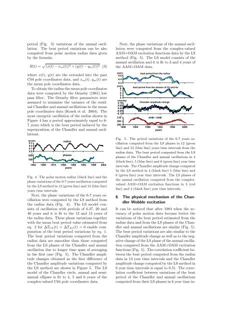
most energetic oscillation of the radius shown in
Figure 4 has a period approximately equal to 6-
7 years which is the beat period induced by the
superposition of the Chandler and annual oscillations.
arcsec
radius
0.3
0.2
0.1
0.0
o
200 phases
180
1962 1968 1974 1980 1986 1992 1998 2004
years
Fig. 4. The polar motion radius (black line) and the
phase variations of the 6-7 years oscillation computed
by the LS method in 12 (green line) and 13 (blue line)
years time intervals.
Next, the phase variations of the 6-7 years oscillation
were computed by the LS method from
the radius data (Fig. 4). The LS model consists
of oscillation with periods of 6.37, 20 and
40 years and it is fit to the 12 and 13 years of
the radius data. These phase variations together
with the mean beat period value estimated from
eq. 2 for ∆T Ch (t) = ∆T An (t) = 0 enable computation
of the beat period variations by eq. 1.
The beat period variations computed from the
radius data are smoother than those computed
from the LS phases of the Chandler and annual
oscillation due to longer time span of averaging
in the first case (Fig. 5). The Chandler amplitude
changes obtained as the first difference of
the Chandler amplitude variations computed by
the LS method are shown in Figure 5. The LS
model of the Chandler circle, annual and semiannual
ellipses is fit to 4, 5 and 6 years of the
complex-valued C04 pole coordinates data.
Next, the phase variations of the annual oscillation
were computed from the complex-valued
AAM+OAM excitation functions data by the LS
method (Fig. 5). The LS model consists of the
annual oscillation and it is fit to 3 and 4 years of
the AAM+OAM data.
years
6.6
beat period from the radius
6.4
6.2
years
8
beat period from the phases of Ch and An
7
6
5
4
mas/day
0.10
Chandler amplitude change
0.05
0.00
-0.05
-0.10
o
310 AAM + OAM
300
290
1980 1984 1988 1992 1996 2000
years
Fig. 5. The period variations of the 6-7 years oscillation
computed from the LS phases in 12 (green
line) and 13 (blue line) years time intervals from the
radius data. The beat period computed from the LS
phases of the Chandler and annual oscillations in 4
(black line), 5 (blue line) and 6 (green line) year time
intervals. The Chandler amplitude change computed
by the LS method in 4 (black line) 5 (blue line) and
6 (green line) year time intervals. The LS phases of
the annual oscillation computed from the complexvalued
AAM+OAM excitation functions in 3 (red
line) and 4 (black line) year time intervals.
6 The physical mechanism of the Chandler
Wobble excitation
It can be noticed that after 1984 when the accuracy
of polar motion data became better the
variations of the beat period estimated from the
radius data and from the LS phases of the Chandler
and annual oscillations are similar (Fig. 5).
The beat period variations are also similar to the
Chandler amplitude change as well as to the negative
change of the LS phase of the annual oscillation
computed from the AAM+OAM excitation
functions (Fig. 5). The correlation coefficient between
the beat period computed from the radius
data in 13 year time intervals and the Chandler
amplitude change computed by the LS method in
6 year time intervals is equal to 0.51. The correlation
coefficient between variations of the beat
period of the Chandler and annual oscillations
computed from their LS phases in 6 year time in-