Chapter 3 Applications
Chapter 3 Applications
Chapter 3 Applications

Create successful ePaper yourself
Turn your PDF publications into a flip-book with our unique Google optimized e-Paper software.
<strong>Chapter</strong> 3<br />
<strong>Applications</strong><br />
Topics covered in SS 2012:<br />
— pumping model behind the master equation for a micromaser<br />
(Sec.3.1.2)<br />
— quantum theory of the laser: elements of the master equation<br />
(Sec.3.1.3)<br />
— photon statistics of the laser (Sec.3.1.4)<br />
— Schawlow–Townes formula for the linewidth of a laser (Sec.3.3)<br />
3.1 Introduction to laser theory<br />
What are the typical components of a laser 1 Without going into details,<br />
we can identify two of them:<br />
• some matter that amplifies light (“active medium”);<br />
• some device that traps the light around the space filled with the<br />
medium (“cavity”)<br />
In order to obtain an amplifying medium, one has to “pump” energy into<br />
it. The gain medium is thus a converter between the pump energy and the<br />
light emission. Quite often, the conversion efficiency is low, with values in<br />
the range 10–50% being considered “large”.<br />
The feedback mechanism is needed because the light would otherwise<br />
escape from the medium. An optical cavity like a Fabry-Pérot resonator<br />
1 Acronym of “Light Amplifier by Stimulated Emission of Radiation”<br />
86
(two mirrors) does this job because the light can travel back and forth<br />
between the mirrors a large number of times.<br />
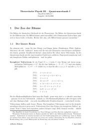
3.1.1 Idea of the theory<br />
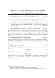
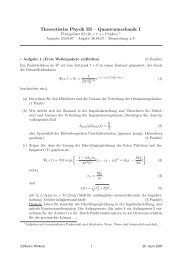
Sargent and Scully (1972) propose the following diagram that relates the<br />
different theories needed to describe a laser.<br />
field<br />
E ( x, t)<br />
Q.M.<br />
atoms<br />
< d (t)><br />
Stat.<br />
matter<br />
P ( x, t)<br />
E.Dyn.<br />
field<br />
E ( x, t)<br />
self-consistency<br />
The electromagnetic field drives microscopic dipoles in the laser<br />
medium. This was the topic of the previous term. A statistical description<br />
gives, implicit in the density matrix approach we followed, links the dipoles<br />
to the macroscopic polarization of the medium [see Eq. (3.19) below]. The<br />
polarization enters the Maxwell equations for the electromagnetic field as<br />
a source and generates the field. In the end, a self-consistent description is<br />
required: the fields at the left and right end should coincide. The condition<br />
of self-consistency allows to derive the following important quantities:<br />
• the laser threshold,<br />
• the laser intensity in steady state,<br />
• the laser frequency.<br />
This can be achieve even when one treats the field treated classically. For<br />
example, a “classical” or “coherent” field appeared via the Rabi frequency<br />
in the Bloch equations of the previous term. This approach is called “semiclassical<br />
laser theory”. Note that nowhere in this approach does the word<br />
“photon” appear (if one is serious).<br />
When a quantum-mechanical description is adopted, the photon finally<br />
comes into play and one may also derive<br />
• the photon number probabability distribution (“photon statistics”),<br />
• the intensity fluctuations and correlations of laser light,<br />
87
• the phase fluctuations (related to the laser linewidth).<br />
We shall illustrate this quantum theory by a calculation of the photon statistics<br />
and the laser linewidth.<br />
We focus in these elementary considerations on a homogeneously distributed<br />
medium in the cavity made up from identical two-level systems<br />
(“homogeneous broadening”). Please refer to the experimental physics lectures<br />
for the discussion of “inhomogeneous” frequency broadening due to,<br />
for example, the atomic motion and other features.<br />
Loss, gain, and nonlinearity. (Material taken from “Laser theory in manifest<br />
Lindblad form” (Henkel, 2007).)<br />
The quantum theory of a laser is a textbook example of a nonlinear<br />
problem that requires techniques from open quantum systems. The key issue<br />
is the nonlinearity in the gain of the laser medium, due to saturation,<br />
that leads to coupled nonlinear equations already at the semiclassical level.<br />
The quantum theory makes things worse by its use of non-commuting operators.<br />
Recall that in the so-called semiclassical theory (see Sec.3.2), the following<br />
equation of motion for the intensity I the laser mode can be derived<br />
(Sargent III & Scully, 1972; Orszag, 2000):<br />
dI<br />
dt = −κI + GI<br />
1 + βI<br />
(3.1)<br />
where κ is the loss rate, G is the linear gain, and β describes gain saturation<br />
for the laser medium. A quantum upgrade of this theory replaces<br />
the intensity by the photon number a † a where the annihilation operator a<br />
describes the field amplitude of the laser mode. Mode loss is easy to handle<br />
by coupling the laser mode linearly to a mode continuum ‘outside’ the laser<br />
cavity (Walls & Milburn, 1994). This leads to a master equation for the<br />
density matrix in so-called Lindblad form [see Eq.()]<br />
dρ<br />
= κ(LρL † − 1<br />
dt ∣ 2 {L† L, ρ}) (3.2)<br />
loss<br />
with a Lindblad operator L loss = √ κ a. Linear gain can be handled in the<br />
same way, taking L gain,0 = √ G a † , but gain saturation is more tricky. A<br />
88
heuristic conjecture is a Lindblad operator L gain = √ G a † (1+βa † a) −1/2 . The<br />
operator ordering can only be ascertained a posteriori, and it is difficult to<br />
choose among the replacements I ↦→ a † a, aa † , or 1 2 {a† a+aa † }. We illustrate<br />
this difficulty in Sec.3.1.3 where the conventional quantum theory of the<br />
laser (due to Scully & Lamb) is presented.<br />
In this section, we start with a microscopic model for the pumping process.<br />
This is motivated by experiments with so-called micromasers where a<br />
(microwave) cavity is crossed by a beam of excited two-level atoms. Nonlinear<br />
gain emerges from a treatment beyond second order in the atomfield<br />
coupling. Orszag (2000); Stenholm (1973) analyze a pumping model<br />
based on a dilute stream of excited two-level atoms that cross the laser<br />
cavity one by one and interact with the laser mode during some randomly<br />
distributed interaction time. This model can be largely handled exactly<br />
(Briegel & Englert, 1993), even in the presence of incoherent effects like<br />
cavity damping, imperfect atom preparation, and frequency-shifting collisions.<br />
The setup has become known as the ‘micromaser’ because of its<br />
experimental realization with a high-quality cavity (Meschede & al., 1985;<br />
Brune & al., 1987; Raizen & al., 1989). One line of research has focused<br />
on the so-called ‘strong coupling regime’ that permits the laser mode to be<br />
driven into non-classical states (Weidinger & al., 1999; Varcoe & al., 2000).<br />
We focus here on the ‘weak coupling’ regime. On the level of the master<br />
equation for the laser mode, this regime corresponds to a small product of<br />
coupling constant and elementary interaction time τ so that one can expand<br />
in this parameter. Mandel & Wolf (1995); Orszag (2000) consider<br />
a coupling to fourth order. For the description of a realistic experiment,<br />
one has to average the master equation with respect to a distribution of<br />
the interaction time τ (Sec. 3.1.2). It turns out, however, that the resulting<br />
master equation is not of the well-known Lindblad form, although it<br />
preserves the trace of the density matrix. This leads to conflicts with the<br />
positivity of the density operator, as is known since the original derivation<br />
of the master equation by Lindblad and by Gorini et al. (Lindblad, 1976;<br />
Gorini & al., 1976). We have shown that this problem can be cured by<br />
adding certain terms in sixth order to the master equation (Henkel, 2007).<br />
The material presented here is based on this reference. This problem provides<br />
us with an example where the Lindblad master equation can be de-<br />
89
ived from the Kraus-Stinespring representation of the finite-time evolution<br />
of the density matrix (Sec. 1.2). The mathematical treatment is at the border<br />
of validity of the formal Lindblad theory since one has to deal with an<br />
infinite-dimensional Hilbert space and continuous sets of Kraus and Lindblad<br />
operators.<br />
3.1.2 The micromaser model<br />
Consider a two-level atom with states |g〉, |e〉 that is prepared at time t in<br />
its excited state |e〉 = (1, 0) T (density matrix ρ A = |e〉〈e|) and that interacts<br />
with a single mode (density matrix ρ) during a time τ. One adopts a Jaynes-<br />
Cummings-Paul Hamiltonian for the atom-field coupling<br />
H JCP = ¯hg ( a † σ + aσ †) , σ = |g〉〈e| =<br />
⎛<br />
⎝ 0 0<br />
1 0<br />
⎞<br />
⎠ (3.3)<br />
(this applies at resonance in a suitable interaction picture). Assume that<br />
the initial density operator of the atom+field-system factorizes into P (t) =<br />
ρ(t) ⊗ ρ A , compute P (t + τ) by solving the Schrödinger equation and get<br />
the following reduced field density matrix (Orszag, 2000; Stenholm, 1973)<br />
ρ(t + τ) = cos(gτ ˆϕ)ρ(t) cos(gτ ˆϕ) + (gτ) 2 a † sinc(gτ ˆϕ)ρ(t) sinc(gτ ˆϕ)a (3.4)<br />
where sinc(x) ≡ sin(x)/x, and ˆϕ 2 = aa † is one plus the photon number<br />
operator. The operator-valued functions cos and sinc are defined by their<br />
series expansion. Only even powers of the argument occur, hence we actually<br />
never face the square root ˆϕ of the operator aa † . In the following, we<br />
abbreviate the mapping defined by Eq.(3.4) by τρ(t) (this is sometimes<br />
called a superoperator).<br />
The operation (3.4) describes an elementary ‘pumping event’ of the<br />
laser. We assume in the following that this event provides only a small<br />
change in the density operator, ( τ − )ρ is ‘small’. To provide a more realistic<br />
description, one introduces the following additional averages: excited<br />
atoms appear in the laser cavity at a rate r such that rτ ≪ 1. Over a time<br />
interval ∆t, a number of r∆t pumping events happens, and the accumulated<br />
change in the density operator is ∆ρ = r∆t( τ − )ρ. This will lead<br />
us to a differential equation when ∆t is ‘small enough’.<br />
90
We make the additional assumption that the interaction time τ is distributed<br />
according to the probability measure dp(τ) with mean value ¯τ.<br />
This reflects the fact that atoms can cross the cavity mode with different<br />
velocities, at different positions etc. Also in a conventional laser, atoms<br />
interact with the laser mode only during some finite (and randomly distributed)<br />
time of the order of the lifetime of the excited state. Keeping<br />
the coarse-grained time step (∆t ≫ ¯τ), we thus get the difference equation<br />
(Orszag, 2000; Stenholm, 1973)<br />
∫<br />
∆ρ<br />
∆t = r dp(τ) ( τ − ) ρ. (3.5)<br />
To simplify the superoperator appearing on the right hand side, Orszag<br />
(2000); Stenholm (1973) suggest an expansion in powers of gτ ˆϕ up to the<br />
fourth order. Using an exponential distribution for dp(τ), this leads to the<br />
approximate master equation<br />
dρ<br />
dt<br />
= G ( a † ρa − 1 2 {aa† , ρ} )<br />
+ B ( 3aa † ρaa † + 1 2 {(aa† ) 2 , ρ} − 2a † {aa † , ρ}a ) (3.6)<br />
where we followed the common practice of interpreting this as a differential<br />
equation. We use {·, ·} to denote the anticommutator. The linear gain<br />
is G = 2r(g¯τ) 2 , and B = (g¯τ) 2 G is a measure of gain saturation. Indeed,<br />
the first line of Eq.(3.6) is in Lindblad form with L gain = √ G a † – applying<br />
this operator increases the photon number by one. It is easy to see that this<br />
leads, on average, to an increasing field amplitude, (d/dt)〈a〉 gain = G〈a〉.<br />
Losses from the laser mode can be included in the usual way by adding<br />
a term of the same structure as the first line of Eq.(3.6), but featuring the<br />
Lindblad operator L loss = √ κ a with the cavity decay rate κ, see Eq.(3.2)<br />
(Orszag, 2000; Stenholm, 1973). The same master equation as Eq.(3.6) is<br />
also found, using a different pumping model (Mandel & Wolf, 1995).<br />
It is easy to check that Eq.(3.6) preserves the trace of ρ, using cyclic permutations.<br />
Nevertheless, it is not of the general form derived by Lindblad<br />
for master equations that preserve the complete positivity of density matrices<br />
(Lindblad, 1976; Gorini & al., 1976; Alicki & Lendi, 1987). We shall<br />
show below [Eq.(3.12)] that Eq.(3.6) indeed leads to a density matrix with<br />
negative probabilities. Of course, one can accept to work with this kind of<br />
91
‘post-Lindblad’ master equations (as they appear frequently in the papers<br />
of Golubev and co-workers, see e.g. Golubev & Gorbachev (1986)). It is<br />
also possible to construct a set of Lindblad operators {L λ } such that with<br />
a few additional terms to the master equation (3.6), it can be brought into<br />
the Lindblad form. For more details, see “Laser theory in manifest Lindblad<br />
form” (Henkel, 2007).<br />
3.1.3 Scully-Lamb master equation<br />
In this section, we outline a theory of the laser that starts from a quantum<br />
description of the cavity field. We still use for simplicity the single mode<br />
approximation — the basic observables are hence the annihilation and creation<br />
operators a, a † for the field mode.<br />
The laser is an open quantum system because energy is continuously fed<br />
into and removed from the cavity mode. We therefore have to use a density<br />
matrix description, as we did in the first part for a two-level atom. What<br />
are the “reservoirs” that the field mode is coupled to First of all, the mode<br />
continuum outside the cavity: part of the cavity losses show up here (and<br />
permit to observe the laser dynamics). But in general, losses also occur in<br />
the material that makes up the cavity: mirrors and optical elements. We<br />
do not develop in this semester’s course a detailed quantum theory of lossy<br />
optical elements (see chapter 4 of the SS 2002 version). Finally, the laser<br />
medium is also a reservoir of energy that may flow into the field mode —<br />
or not when the medium spontaneously emits photons into other modes.<br />
In this section, we recall the master equation description for linear cavity<br />
loss and motivate the corresponding model for the gain medium. We<br />
shall derive a rate equation for the probabilities of finding n photons in the<br />
laser mode whose stationary solution gives the photon statistics. Finally, a<br />
sketch is given of the Schawlow-Townes limit for the laser linewidth.<br />
Cavity damping<br />
The density operator for the cavity field, ρ(t), acts on the Hilbert space for<br />
the harmonic oscillator associated with the field mode. Taking the trace,<br />
we find the quantum expectation values of the quantities of interest. The<br />
average electric field, for example, is given by (we only write the positive<br />
92
frequency part)<br />
〈E(x, t)〉 = ef(x)E 1 〈a(t)〉 = ef(x)E 1 tr [a ρ(t)]<br />
The trace can be performed in any basis, using photon number states or<br />
coherent states, for example. In the absence of any interaction, the Heisenberg<br />
operator a evolves freely at the frequency ω c of the cavity. (We suppose<br />
for simplicity that this coincides with the laser frequency.)<br />
We have seen in chap. 1 that the master equation to describe linear<br />
damping can be written in terms of Lindblad or jump operators. The one<br />
we need for cavity damping is given by L = √ κ a, leading to<br />
dρ<br />
= κ aρa † − κ {<br />
dt ∣ a † a, ρ } . (3.7)<br />
damp<br />
2<br />
It is easy to check that the rate κ has the same meaning as in the semiclassical<br />
theory: it gives the (exponential) decay of the field’s photon number<br />
if no other dynamics is present.<br />
As an exercise, you may want to derive the rate equations for the diagonal<br />
elements p n (t) = 〈n|ρ(t)|n〉 of the density matrix (these form the<br />
‘photon statistics’). The master equation (3.7) gives a transition rate between<br />
the photon number states |n〉 and |n − 1〉 that is given by nκ, proportional<br />
to the number of photons that are presently in the cavity mode.<br />
One is tempted to interpret this as “each photon decides independently to<br />
leave the cavity.” The final state is the vacuum state with zero photons —<br />
this is related to the implicit assumption that the reservoir is at zero temperature.<br />
It is a reasonable approximation at optical frequencies and room<br />
temperature.<br />
Gain<br />
In the previous semester, we used a model with a driven field mode where<br />
a “pump” generates a coherent state. We cannot use this model any longer<br />
because the laser medium does not provide, a priori, a fixed phase reference<br />
for the field it generates. At least the spontaneous emission of the pumped<br />
two-level atoms is “incoherent” (no fixed phase).<br />
93
A suitable model for cavity gain in the linear regime is given by the jump<br />
operator L 2 = √ G a † and the master equation<br />
dρ<br />
= G a † ρa − G {<br />
aa † , ρ } , (3.8)<br />
dt ∣ gain<br />
2<br />
where G is the gain rate coefficient and, up to the exchange of a and a † , no<br />
sign changes occur.<br />
What about gain saturation It is included in this theory if we allow G<br />
to depend on the instantaneous intensity of the cavity mode. The gain thus<br />
depends on the photon number, G = G(n). By analogy to the semiclassical<br />
gain, one can use the model<br />
G(a † a) =<br />
G 0<br />
1 + Ba † a<br />
where 1/B plays the role of a saturation photon number. This actually leads<br />
to complications in the construction of suitable Lindblad operators. (How<br />
to take the square root here) There are examples in textbooks that work<br />
with non-Lindblad forms and that need to be corrected afterwards to avoid<br />
unphysical results like negative probabilities.<br />
3.1.4 Photon statistics<br />
To start our analysis, let us compute the rate equations for the populations<br />
p n ≡ ρ nn of finding n photons in the cavity mode. The sum of damping and<br />
gain gives the master equation<br />
dρ<br />
dt = −iω [<br />
c a † a, ρ ] − κ {<br />
a † a, ρ } + κ aρa †<br />
2<br />
− G(a† a) {<br />
aa † , ρ } + G(a † a) a † ρa. (3.9)<br />
2<br />
Taking the expectation value in the state |n〉 of the master equation (3.9),<br />
we get<br />
dp n<br />
dt = −nκ p n + (n + 1)κ p n+1 − (n + 1)G(n) p n + nG(n − 1) p n−1 (3.10)<br />
From the terms with a negative sign, we see that transitions leave the state<br />
|n〉 with rates nκ and (n+1)G(n). Looking at the rate equation for the state<br />
94
|n − 1〉, we see that population from state |n〉 arrives at a rate nκ. We have<br />
thus identified a first process: the cavity field loses one photon at the rate<br />
nκ. This is the expected loss process. But there is also a transition from<br />
|n〉 to |n + 1〉, occurring at a rate (n + 1)G(n). This is both spontaneous<br />
(“+1”) and stimulated emission (“n”) from the laser medium. Note that<br />
the present theory requires G to be positive (inverted medium) because<br />
transition rates are positive. The dependence of G(n) on the photon number<br />
again models the gain saturation, as was the case in the semiclassical<br />
theory.<br />
• Van Kampen’s trick with the two-term recurrence relation Kampen<br />
(1960).<br />
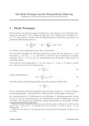
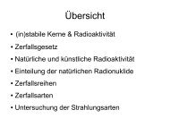
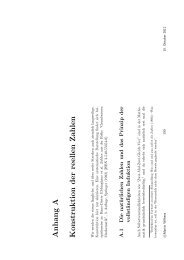
The transitions we have found are summarized in figure 3.1. We can<br />
| n+1 ><br />
(n+1) κ<br />
(n+1)G(n)<br />
| n ><br />
n κ<br />
nG(n-1)<br />
| n -1><br />
Figure 3.1: Transitions between photon number states.<br />
now determine the stationary state of the laser. The probabilities p n and<br />
p n+1 , say, then do not change with time, and therefore the probability current<br />
for the loss process |n + 1〉 → |n〉 must be equal to the current for the<br />
emission process |n〉 → |n + 1〉:<br />
(n + 1)κp n+1 = (n + 1)G(n)p n (3.11)<br />
For the pair of levels |n〉 and |n − 1〉, we get nκp n = nG(n − 1)p n−1 from<br />
the rate equation (3.10) which can also be found by shifting the label n<br />
in Eq.(3.11). We can check for the special case |0〉 ↔ |1〉 that there is no<br />
95
saturation effect for the spontaneous emission rate into the empty cavity,<br />
which seems perfectly reasonable. 2<br />
We observe that the dynamic equilibrium between loss and gain processes<br />
gives a recurrence relation for the photon number probabilities in<br />
the stationary state. It is easily solved to give<br />
p n+1 = G(n)<br />
κ<br />
p n ⇒ p n = N<br />
n−1 ∏<br />
m=0<br />
G(m)<br />
κ<br />
= N<br />
( G0<br />
κ<br />
) n n−1 ∏ 1<br />
m=0<br />
1 + Bm , (3.12)<br />
where N is a normalization constant. Below threshold, G 0 < κ, each of<br />
the ratios G(n)/κ is smaller than unity, and the most probable state is the<br />
vacuum — perfectly reasonable because the laser intensity is damped away.<br />
Above threshold and for weak saturation, G(n)/κ ≈ G 0 /κ > 1, and photon<br />
numbers larger than zero are favoured. The maximum of the distribution<br />
is reached at a photon number n max where G(n max )/κ = 1. This equation<br />
can be solved to give<br />
n max = G 0 − κ<br />
κB<br />
which looks very similar to the steady state intensity of the semiclassical<br />
theory.<br />
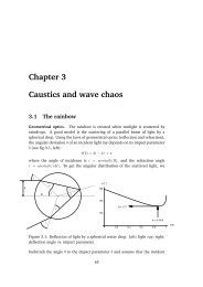
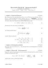
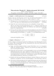
The photon statistics (3.12) is plotted in figure 3.2 for a laser below and<br />
above threshold. Note that below threshold, we do not have a thermal state<br />
(the probability is not an exponential ∝ e −βn¯hωc ), and that above threshold,<br />
the width of the number distribution is larger than for a coherent state with<br />
the same most probable photon number.<br />
As an exercise, you can use the following representation of the product<br />
in (3.12)<br />
n−1 ∏<br />
m=0<br />
1<br />
1 + Bm = Γ(1/B)<br />
B−n<br />
Γ(1/B + n)<br />
where Γ(·) is now the gamma function. Using the Stirling formula for large<br />
values of n and 1/B, show that p n has the form of a truncated gaussian<br />
distribution and compute its width. You will find that the width approaches<br />
that of a coherent state,<br />
∆n 2 → n max<br />
2 There are high Q cavity experiments where the field of a single photon suffices to<br />
saturate an atomic transition.<br />
96
elow threshold<br />
0.04<br />
above threshold<br />
10 0 photon number n<br />
10 −1<br />
G = 0.9 κ<br />
B = 0.01<br />
0.035<br />
0.03<br />
0.025<br />
G = 1.1 κ<br />
B = 0.001<br />
laser<br />
coherent state<br />
p n<br />
p n<br />
0.02<br />
10 −2<br />
0.015<br />
0.01<br />
0.005<br />
10 −3<br />
0 5 10 15 20<br />
0<br />
0 50 100 150 200 250<br />
photon number n<br />
Figure 3.2: Photon statistics of a laser in steady state. Left: below threshold<br />
G ≡ G 0 < κ, right: above threshold.<br />
when the laser is operating far above threshold. (This is difficult to achieve<br />
in practice, however.)<br />
3.2 Semiclassical laser theory<br />
Material not covered in SS 2012. We expose here, mainly for informative purposes,<br />
the so-called semiclassical theory of the laser.<br />
3.2.1 Wave equation for the field<br />
We start with a reminder of the electrodynamics in a material with a given polarization.<br />
Let us recall that the polarization field enters the following Maxwell<br />
equation:<br />
1<br />
µ 0<br />
∇ × B = j + ∂ ∂t (ε 0E + P)<br />
where it gives the “bound” part of the current density. We put in the following the<br />
“free” current density j = 0 because we assume that the active material is globally<br />
neutral and the light only induces dipoles in it. Combining with the Faraday induction<br />
equation, ∇ × E = −∂ t B, one gets the wave equation for the electric field<br />
where the polarization enters as a source term:<br />
∇ × ∇ × E + 1 c 2 ∂ 2<br />
∂ 2<br />
∂t 2 E = −µ 0 P. (3.13)<br />
∂t2 We now make the approximation that in the cavity, a single mode is sufficient to<br />
capture the field dynamics. You have seen that one can then write for the field<br />
97
operator<br />
]<br />
E(x, t) = eE 1<br />
[f(x)a(t) + f ∗ (x)a † (t)<br />
(3.14)<br />
where E 1 = (¯hω L /2ε 0 V ) 1/2 is the “one-photon field amplitude”, a(t) is the annihilation<br />
operator for the mode (time-dependent in the Heisenberg picture), and<br />
f(x) is the spatial mode function. It solves the homogeneous equation<br />
∇ × ∇ × ef − ω2 c<br />
ef = 0 (3.15)<br />
c2 as you remember from the field quantization procedure. Here ω c is one of the<br />
(empty) cavity resonance frequencies. For a planar cavity with axis along the z-<br />
direction, for example, we have<br />
f(x) = √ 2 sin(kz) (3.16)<br />
with k = nπ/L = ω c /c where n is a positive integer and L the cavity length.<br />
This mode function is normalized such that the integral of its square over the<br />
cavity volume V gives V . There are also lasers where propagating modes are<br />
a suitable description. In the photonics lectures, other cavity modes, including<br />
their transverse behaviour (perpendicular to the cavity axis) are introduced. For<br />
the semiclassical theory we develop here first, the product E 1 a(t) = E(t) gives<br />
the (positive frequency) field amplitude. Its absolute square corresponds to the<br />
intensity, with a ∗ (t)a(t) giving the “photon number” (although this is not required<br />
to be an integer in the semiclassical theory).<br />
We now project the wave equation (3.13) onto the field mode ef(x). The<br />
term involving f ∗ (x)a † (t) does not contribute when a propagating mode is used.<br />
We also make the approximation of slowly varying amplitudes for E(t) that oscillates<br />
essentially at the frequency ω L . The polarization field as well, P(x, t) =<br />
P(x) e −iωLt +c.c. This means that the time derivative of P(x) is much smaller than<br />
ω L P(x). (With this approximation and standing wave modes, the term f ∗ (x)a(t)<br />
drops out at this point.) We get<br />
Ė = −i(ω L − ω c )E − κ 2 E + i ω L<br />
2ε 0<br />
∫ d 3 x<br />
V f ∗ (x)e · P(x), (3.17)<br />
where ω L − ω c is the frequency detuning with respect to the cavity resonance<br />
and V the cavity volume. We have introduced the phenomenological decay rate<br />
κ for the energy of the cavity field. The quality factor of the cavity (often known<br />
experimentally) is given by Q = ω c /κ. Notice that the spatial integral is the overlap<br />
of the polarization field with the cavity mode. It is easy to see from this equation<br />
that the real part of the polarization P determines a frequency shift of the laser<br />
98
(with respect to the cavity frequency), and that its imaginary part changes the<br />
energy ∝ |E| 2 of the field. In particular, if Im P is negative, the field energy<br />
increases (emission). We thus anticipate to find the absorption and emission of<br />
the medium in the imaginary part of the polarization.<br />
3.2.2 Dipole moment and polarization<br />
The “active medium” cavity inside the cavity that provides the polarization consists,<br />
in many cases, of a large number of atoms or molecules. These atoms are<br />
prepared in the excited state by some process that feeds energy into them (“pumping<br />
mechanism”), and then wait to release their energy in the form of photons<br />
into the cavity field. A two-level approximation for the atoms is a simple way to<br />
account for the sharp, nearly monochromatic emission spectrum of the laser. We<br />
could have used as well a harmonic oscillator 3 , however, this does not reproduce<br />
some basic features of the laser like gain saturation. The quantum theory for the<br />
atom-light interaction gives us an expression for the “microscopic”, average electric<br />
dipole 〈d(t)〉. The polarization field is then simply the number density of these<br />
dipoles<br />
P(x, t) = N(x)〈d(t)〉. (3.18)<br />
In general, the density N(x) is position dependent. In fact, also the induced dipole<br />
is because it involves the light field at the position x.<br />
The complex, slowly varying polarization field can be connected to the coherences<br />
of the density matrix in the rotating frame:<br />
[<br />
]<br />
P(x, t) = N(x) 〈d (+) (t)〉 + c.c.<br />
[<br />
]<br />
= N(x)d ρ eg (t)e −iωLt + c.c.<br />
(3.19)<br />
where d (+) (t) is the positive frequency part of the atomic dipole operator, d is<br />
the fixed vector of dipole matrix elements and ρ eg (t) is the off-diagonal element<br />
(“optical coherence”) of the atomic density matrix in the frame rotating at ω L . A<br />
formula like (3.19) assumes that all dipoles in the medium are driven by a similar<br />
field and do not interact with each other. This is a first starting point and leaves<br />
place for more elaborate theories, of course. We assume in particular that the<br />
resonance frequency is the same for all microscopic dipoles. This is not true for<br />
atoms in a (thermal) gas where the Doppler effect leads to a distribution of the<br />
resonance frequencies (“inhomogeneous broadening”).<br />
3 This is a good model for antennas emitting at radio frequencies.<br />
99
p<br />
"<br />
e<br />
e<br />
!<br />
p<br />
!<br />
#<br />
0<br />
"<br />
g<br />
g<br />
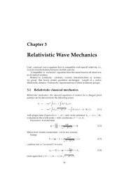
Figure 3.3: Four-level model to describe incoherent population pumping of<br />
the upper state e of the lasing transition e ↔ g.<br />
3.2.3 Dipole moment and atomic inversion<br />
We now have to find a way to determine the dipole moment of the two-level atoms.<br />
Recall that its imaginary part is essential for light amplification. We shall see that it<br />
depends on the atomic inversion (population difference between upper and lower<br />
state). To this end, we use the optical Bloch equations for the atomic density<br />
matrix, with some modifications by adding additional energy levels. This model<br />
also provides a better understanding of the “pumping” mechanism, beyond some<br />
phenomenological rate equations. The modified two-level system is for example<br />
a four-level atom with fast relaxation in the two upper and two lower states. A<br />
simple model with four states as shown in figure 3.3 is outlined in the exercises. In<br />
this limit, the optical Bloch equations can be simplified, and one gets a justification<br />
for the often-used rate equations.<br />
The next task is to compute the optical coherence ρ eg (t) from the optical Bloch<br />
equations. Let us write down these equations for the two levels e and g involved<br />
in the laser transition. The rate equations for the populations ρ ee and ρ gg involve<br />
a pumping rate λ e = Γ e ρ pp into the upper state (via rapid decay from the pumped<br />
state p), the spontaneous decay rate γ and a decay rate Γ g for the lower state.<br />
Including the Rabi frequency Ω = −(2/¯h)d · E for the laser field, as you have<br />
learned in the previous semester, this gives<br />
˙ρ ee = λ e − γρ ee + i Ω 2 (ρ eg − ρ ge ) , (3.20)<br />
˙ρ gg = γρ ee − Γ g ρ gg − i Ω 2 (ρ eg − ρ ge ) . (3.21)<br />
Notice that the first equation gives an increase of the excited state population<br />
when the coherence ρ eg has a positive imaginary part (recall that Ω is actually<br />
100
negative. . . ). This is in agreement with the damping of the field energy in the<br />
wave equation derived before.<br />
The last Bloch equation is for the coherence itself. The population decay rates γ<br />
and Γ g lead to a decoherence rate Γ = 1 2 (γ +Γ g) as you have seen in the derivation<br />
of the Bloch equations. In the frame rotating at the laser frequency ω L , the laser<br />
field detuning is ∆ = ω L − ω eg , and we get<br />
˙ρ eg = i∆ρ eg − Γρ eg + i Ω 2 (ρ ee − ρ gg ) . (3.22)<br />
From this equation we learn that the optical dipole is created by the population<br />
difference (inversion) ρ ee − ρ gg . As discussed in the exercises, this equation can be<br />
solved approximately in the limit that the decay rate Γ is the largest time constant<br />
around (this solution also corresponds to the stationary state):<br />
ρ eg = − Ω/2<br />
∆ + iΓ (ρ ee − ρ gg ) . (3.23)<br />
In particular, the imaginary part of the optical coherence is (we assume as usual a<br />
real Rabi frequency)<br />
Im ρ eg =<br />
ΓΩ/2<br />
∆ 2 + Γ 2 (ρ ee − ρ gg ) .<br />
Note that this expression is negative when the two-level system is inverted (upper<br />
level population ρ ee > ρ g ), using again that actually Ω < 0. This means that the<br />
medium amplifies the light via stimulated emission.<br />
3.2.4 Medium polarization and saturation<br />
Solving also the other Bloch equations in the stationary state, we can compute the<br />
inversion<br />
∆ 2 + Γ 2<br />
ρ ee − ρ gg = λ e (1/γ − 1/Γ g )<br />
∆ 2 + Γ 2 + (Γ/γ)Ω 2 /2 . (3.24)<br />
The system is inverted when the lifetime 1/γ of the upper state exceeds the lifetime<br />
1/Γ g of the lower state, which is perfectly reasonable.<br />
The end result of the calculation is the following expression for the polarization<br />
field. We quote only the amplitude of the positive frequency component and<br />
assume that dipole moment and electric field are collinear:<br />
P(x) = N(x)(D 2 λ e (1/γ − 1/Γ g ) (∆ − iΓ)<br />
/¯h)eE(x)<br />
∆ 2 + Γ 2 + 2(ΓD 2 /γ¯h 2 (3.25)<br />
)|E(x)| 2<br />
=:<br />
ε 0 χE(x)<br />
1 + B|E(x)| 2 . (3.26)<br />
101
In the last line, we have introduced the (linear) susceptibility χ of the laser<br />
medium and a coefficient B that takes into account the nonlinear response.<br />
The most important result is that the imaginary part of the polarization is<br />
negative (amplification of the field) when the two-level system is inverted. The<br />
four-level scheme shown in fig. 3.3 is just one possibility to achieve inversion by<br />
a suitable pumping scheme. Refer to the experimental physics lectures for other,<br />
perhaps more efficient, pumping mechanisms.<br />
The coefficient B in (3.26) describes the saturation of the medium: for very<br />
large laser intensity |E| 2 , the induced polarization decreases proportional to 1/|E|<br />
instead of increasing. The physics behind saturation is characteristic for the twolevel<br />
system: when the laser field gets extremely strong, the inversion vanishes<br />
(see Eq. (3.24)). We have already seen this behaviour when we considered Rabi<br />
oscillations with weak damping: the two-level system gets always re-excited by<br />
the laser and is finally with equal probability in the upper and lower states. For a<br />
harmonic oscillator, there is no saturation since arbitrarily high lying states can be<br />
populated.<br />
3.2.5 Laser threshold and steady state<br />
We now want an equation for the intensity I(t) = |E(t)| 2 (restoring a slow timedependence)<br />
in the mode ef(x). To this end, we work out the spatial overlap in<br />
Eq. (3.17) with a standing wave mode f(x) = √ 2 sin kz:<br />
Ė = −i(ω L − ω c )E − κ ∫<br />
2 E + iω Lχ dz<br />
2 E(t) 2 sin 2 (kz)<br />
L 1 + 2B|E(t)| 2 sin 2 (kz)<br />
Here, L is the cavity length. The difficulty is the sine function in the denominator.<br />
In the exercises, you are asked to compute this integral analytically. Here,<br />
we adopt an approximate treatment that is also often used in the literature and<br />
assume that the saturation is weak. The denominator can then be expanded, and<br />
to first order in B, we get<br />
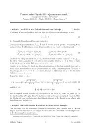
∫ dz [<br />
]<br />
L 2 sin2 (kz) 1 − 2B|E(t)| 2 sin 2 (kz) = 1 − 3B 2 |E(t)|2<br />
As an exercise, you can estimate the dimensionless quantity B|E(t)| 2 for typical<br />
parameter values. This result is often “resummed” to make the saturation effect<br />
more clear:<br />
1 − 3B 1<br />
2 |E(t)|2 ≈<br />
1 + 3B 2 |E(t)|2<br />
102
1<br />
0.8<br />
small saturation<br />
exact<br />
"resummation"<br />
0.6<br />
0.4<br />
0.2<br />
0<br />
0 0.5 1 1.5 2<br />
B |E| 2<br />
Figure 3.4: Different approximations for the gain saturation factor, integrated<br />
over the cavity mode.<br />
This procedure may seem strange, but reproduces quite well the exact result, as<br />
shown in figure 3.4.<br />
The equation of motion for the intensity is now given by (for small gain saturation;<br />
check that B is real)<br />
(<br />
dI<br />
dt = 2 Re E ∗ dE )<br />
= −κI(t) − ω L (Im χ)I(t) [1 − (3B/2)I(t)]<br />
dt<br />
This form suggests the introduction of an amplification rate (“gain”) G =<br />
−ω L (Im χ). Using also the conventional notation β = 3GB/2 (a rate per intensity)<br />
for the saturation coefficient, we obtain<br />
dI<br />
dt = (G − κ)I − βI2 (3.27)<br />
as the fundamental equation of motion for the laser emission.<br />
Threshold<br />
The laser threshold is reached when the gain is sufficiently large to amplify the laser<br />
intensity: G > κ. In this case, stimulated emission overcomes the loss of the field<br />
due to cavity imperfections etc. If the gain is too small (or even negative), G < κ,<br />
then the field decays exponentially from its initial value. This remark points to a<br />
weakness of the semiclassical approach. It is in fact experimentally known that,<br />
once the laser is above threshold (gain exceeds loss), the laser field builds up —<br />
although one starts from an apparently empty cavity. What happens is that the<br />
103
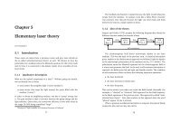
I ss<br />
κ<br />
G<br />
Figure 3.5: Intensity of laser emission vs. gain. The laser threshold is at<br />
G = κ where κ is the loss rate. Solid line: semiclassical theory (3.28). The<br />
dotted line results from the quantum theory.<br />
spontaneous emission of the laser medium “ignites” the exponential growth of the<br />
laser field. But a model for this requires a quantum treatment of the laser, as we<br />
shall outline in the next session.<br />
Steady state intensity<br />
Once the laser is above threshold, the field does not grow indefinitely: the saturation<br />
of the medium, described by the coefficient β, stops the exponential growth.<br />
A steady state is reached at an intensity<br />
I ss = G − κ .<br />
β<br />
This expression is valid not too far above threshold where the expansion of the<br />
saturation denominator is still accurate. Note that this increases linearly with the<br />
gain which is itself proportional to the pumping power. A typical diagram is shown<br />
in figure 3.5 where the steady state intensity is plotted vs. gain. Experimentalists<br />
often use instead of G the pump power.<br />
Phase transition analogy<br />
To summarize, the laser intensity in steady state above and below threshold is<br />
given by<br />
⎧<br />
⎪⎨ 0 if G < κ,<br />
I ss = G − κ<br />
(3.28)<br />
⎪⎩ if G > κ.<br />
β<br />
104
It has been noted that this behaviour is analogous to a phase transition: as a “control<br />
parameter” (gain, temperature) is scanned across a critical value, an “order<br />
parameter” (laser intensity, magnetization, long-range order) abruptly changes to<br />
a nonzero value. This way of thinking has been explored in depth in the school<br />
of H. Haken (Stuttgart), see, e.g., Light, vol. 2 (North-Holland, Amsterdam 1985),<br />
Synergetics (Springer, Berlin 1977), and The Theory of Coherence, Noise and Photon<br />
Statistics of Laser Light, chap. A3 in Laser Handbook, vol. 1, edited by F. T. Arecchi<br />
and E. O. Schulz-DuBois (North-Holland, Amsterdam 1972).<br />
Other topics of semiclassical laser theory<br />
These questions are deferred to other lectures:<br />
• time evolution of the laser intensity (“relaxation oscillation”) and chaos<br />
(“Lorenz model”)<br />
• stability analysis of the above threshold solution I ss = 0.<br />
• inclusion of “inhomogeneous broadening” (dipoles in motion, distribution<br />
of transition frequencies, etc.)<br />
• alternative pumping schemes (incoherent pumping, current injection and<br />
laser diodes etc.)<br />
• multi-mode operation, frequency locking of different modes, “Q-switching”<br />
etc.<br />
Exercises<br />
Find reasonable values for the parameters gain G, cavity loss κ and saturation<br />
coefficient B. An often used quantity is the “saturation intensity” I sat = 1/B. It<br />
gives the typical order of magnitude for the intra-cavity field.<br />
Compute the laser frequency shift with respect to the cavity resonance ω c (rederive<br />
carefully the wave equation) and the medium resonance ω eg .<br />
Plot the gain spectrum (as a function of ω L ) for different laser powers |E| 2 . At<br />
low power, you find a lorentzian whose width is given by the “dephasing rate” Γ<br />
(the relaxation rate of the optical dipole); at high power, the width increases —<br />
this is called “power broadening”.<br />
Try to solve the time-dependent nonlinear equation of motion (3.27), if nothing<br />
else works, at least numerically. How does one reach the steady state Do the<br />
initial conditions matter<br />
105
3.3 Laser linewidth and phase diffusion<br />
We now have to find an expression for the phase diffusion coefficient.<br />
To this end, we shall derive an equation similar to the diffusion equation<br />
(2.23). Since this equation deals with a distribution function for the<br />
phase, it seems natural to introduce a (quasi-)probability distribution for<br />
the laser amplitude. In the last semester, we learned that the P -function<br />
does this job: P (α, α ∗ ) gives the (quasi-)probability that a coherent state<br />
|α〉 occurs in an expansion of the density operator in the basis of coherent<br />
states:<br />
∫<br />
ρ = d 2 α P (α, α ∗ )|α〉〈α|. (3.29)<br />
What is the equation of motion for this distribution From the results of<br />
the last semester, you can show that the following replacement table holds<br />
when the photon operators act on the projector |α〉〈α|<br />
aρ ↦→ αP (3.30)<br />
(<br />
a † ρ ↦→ α ∗ − ∂ )<br />
P<br />
∂α<br />
(<br />
ρa ↦→ α −<br />
∂ )<br />
P<br />
∂α ∗<br />
ρa † ↦→ α ∗ P.<br />
The equation resulting from (3.9) is<br />
∂<br />
∂t P (α, α∗ ) = 1 { ∂<br />
(κ − G)α +<br />
∂<br />
}<br />
2 ∂α ∂α (κ − ∗ G)α∗ P<br />
+ G ∂ 2<br />
P, (3.31)<br />
4 ∂α ∂α∗ where we have yet neglected gain saturation. (The derivatives act on everything<br />
to their right, including P .) An approximate way to take it into<br />
account is to replace G ↦→ G(|α| 2 ) = G 0 /(1 + B|α| 2 ). This is actually an approximation<br />
because when transforming to the P -representation, one has<br />
to neglect some second order and higher order derivatives.<br />
Let us note that the second-order derivative ∂ α ∂ α ∗ in Eq.(3.31) is directly<br />
related to the fact that in the quantum description, the operators a<br />
and a † do not commute. (Their action on a coherent state cannot reduce to<br />
106
multiplication with the numbers α and α ∗ , but must involve some derivative,<br />
as seen in the replacement rules (3.30)). We already suspect that the<br />
second-order derivative may have to do with phase diffusion. We see here<br />
that it is connected to the discrete nature of the photons. Sometimes, people<br />
develop the picture that each photon that is spontaneously emitted by<br />
the gain medium contributes to the cavity field a kind of “one-photon field”<br />
whose phase is arbitrary. The amplitude of the cavity field thus performs<br />
a “random walk” in phase space together with a “deterministic” increase<br />
related to “stimuled emission” where the additional photons add up “in<br />
phase” with the field.<br />
We now have with (3.31) a partial differential equation for a phase<br />
space distribution. It features second-order derivatives like the simple diffusion<br />
equation (2.23). Since we are interested in phase diffusion, it seems<br />
natural to use polar coordinates α = r e iφ . You are asked to make this<br />
transformation in the exercises and to derive the result<br />
∂<br />
∂t P (r, φ) = 1 ∂<br />
2r ∂r r2 (κ − G(r 2 ))P + G(r2 )<br />
4r<br />
( ∂<br />
∂r r ∂ ∂r + 1 r<br />
∂ 2 )<br />
P. (3.32)<br />
∂φ 2<br />
The steady state solution of this equation does not depend on the phase,<br />
but only on the modulus r of the laser amplitude. In the weak saturation<br />
limit where G(r 2 ) ≈ G 0 (1 − Br 2 ), it is given by<br />
P ss (r) ≈ N exp<br />
[<br />
− B 2<br />
(<br />
r 2 − G 0 − κ<br />
G 0 B<br />
This shows a maximum at r 2 max = n max = (G 0 − κ)/G 0 B where we recover<br />
the formula for the semiclassical steady-state intensity (up to a conversion<br />
factor between intensity and photon number). From this distribution, one<br />
can check that the fluctuations of the laser intensity (and the field’s modulus)<br />
are small in the limit 1/B ≫ 1 (large photon number on average,<br />
meaning high above threshold). We can thus confirm that if there are fluctuations,<br />
they occur dominantly in the phase of the field.<br />
With this argument, we can go back to the diffusion equation (3.32)<br />
and identify the phase diffusion coefficient:<br />
) 2<br />
]<br />
.<br />
D = G(r2 )<br />
4r 2<br />
≈ G(n max)<br />
4n max<br />
. (3.33)<br />
107
This formula has been derived first in the 1960/70’s by Schawlow and<br />
Townes. It shows that phase diffusion (and the laser linewidth), well above<br />
threshold, decreases inversely proportional to the laser intensity. When the<br />
gain is increased, the emission spectrum thus shows an ever growing peak<br />
close to the frequency of the cavity mode, that becomes narrower and narrower.<br />
This behaviour is often taken as an experimental proof that a laser<br />
is operating.<br />
108
Bibliography<br />
R. Alicki & K. Lendi (1987). Quantum Dynamical Semigroups and <strong>Applications</strong>,<br />
volume 286 of Lecture Notes in Physics. Springer, Heidelberg.<br />
S. M. Barnett & S. Stenholm (2001). Hazards of reservoir memory, Phys.<br />
Rev. A 64 (3), 033808.<br />
G. Boedecker, C. Henkel, C. Hermann & O. Hess (2004). Spontaneous<br />
emission in photonic structures: theory and simulation, in K. Busch, S.<br />
Lölkes, R. Wehrspohn & H. Föll, editors, Photonic crystals – advances in<br />
design, fabrication and characterization, chapter 2. Wiley-VCH, Weinheim<br />
Berlin.<br />
M. Born & E. Wolf (1959). Principles of Optics. Pergamon Press, Oxford,<br />
6th edition.<br />
H.-P. Breuer & F. Petruccione (2002). The Theory of Open Quantum Systems.<br />
Oxford University Press, Oxford.<br />
H.-J. Briegel & B.-G. Englert (1993). Quantum optical master equations:<br />
The use of damping bases, Phys. Rev. A 47, 3311–3329.<br />
M. Brune, J. M. Raimond, P. Goy, L. Davidovich & S. Haroche (1987). Realization<br />
of a two-photon maser oscillator, Phys. Rev. Lett. 59 (17), 1899–<br />
902.<br />
H. B. Callen & T. A. Welton (1951). Irreversibility and generalized noise,<br />
Phys. Rev. 83 (1), 34–40.<br />
G. Chen, D. A. Church, B.-G. Englert, C. Henkel, B. Rohwedder, M. O. Scully<br />
& M. S. Zubairy (2006). Quantum Computing Devices: Principles, Designs<br />
and Analysis. Taylor and Francis, Boca Raton, Florida.<br />
109
R. Davidson & J. J. Kozak (1971). Relaxation to Quantum-Statistical Equilibrium<br />
of the Wigner-Weisskopf Atom in a One-Dimensional Radiation<br />
Field. III. The Quantum-Mechanical Solution, J. Math. Phys. 12 (6), 903–<br />
917.<br />
T. Dittrich, P. Hänggi, G.-L. Ingold, B. Kramer, G. Schön & W. Zwerger<br />
(1998). Quantum transport and dissipation. Wiley-VCH, Weinheim.<br />
W. Eckhardt (1984). Macroscopic theory of electromagnetic fluctuations<br />
and stationary radiative heat transfer, Phys. Rev. A 29 (4), 1991–2003.<br />
A. Einstein (1905). Über die von der molekularkinetischen Theorie<br />
der Wärme geforderte Bewegung von in ruhenden Flüssigkeiten suspendierten<br />
Teilchen, Ann. d. Physik, Vierte Folge 17, 549–560.<br />
A. Einstein (1917). Zur Quantentheorie der Strahlung, Physik. Zeitschr. 18,<br />
121–128.<br />
Y. M. Golubev & V. N. Gorbachev (1986). Formation of sub-Poisson light<br />
statistics under parametric absorption in the resonante medium, Opt.<br />
Spektrosk. 60 (4), 785–87.<br />
V. Gorini, A. Kossakowski & E. C. G. Sudarshan (1976). Completely positive<br />
dynamical semigroups of N-level systems, J. Math. Phys. 17 (5), 821–25.<br />
R. Hanbury Brown & R. Q. Twiss (1956). Correlation between photons in<br />
two coherent beams of light, Nature 177 (4497), 27–29.<br />
C. Henkel (2007). Laser theory in manifest Lindblad form, J. Phys. B: Atom.<br />
Mol. Opt. Phys. 40, 2359–71.<br />
C. H. Henry & R. F. Kazarinov (1996). Quantum noise in photonics, Rev.<br />
Mod. Phys. 68, 801.<br />
J. D. Jackson (1975). Classical Electrodynamics. Wiley & Sons, New York,<br />
second edition.<br />
N. G. V. Kampen (1960). Non-linear thermal fluctuations in a diode, Physica<br />
26 (8), 585–604.<br />
110
G. Lindblad (1976). On the generators of quantum dynamical semigroups,<br />
Commun. Math. Phys. 48, 119–130.<br />
L. Mandel & E. Wolf (1995). Optical coherence and quantum optics. Cambridge<br />
University Press, Cambridge.<br />
D. Meschede, H. Walther & G. Müller (1985). One-Atom Maser, Phys. Rev.<br />
Lett. 54 (6), 551–54.<br />
M. A. Nielsen & I. L. Chuang (2000). Quantum Computation and Quantum<br />
Information. Cambridge University Press, Cambridge.<br />
L. Novotny & B. Hecht (2006). Principles of Nano-Optics. Cambridge University<br />
Press, Cambridge, 1st edition.<br />
M. Orszag (2000). Quantum Optics – Including Noise Reduction, Trapped<br />
Ions, Quantum Trajectories and Decoherence. Springer, Berlin.<br />
G. M. Palma, K.-A. Suominen & A. K. Ekert (1996). Quantum computers<br />
and dissipation, Proc. Roy. Soc. Lond. A 452, 567–84.<br />
P. Pechukas (1994). Reduced dynamics need not be completely positive,<br />
Phys. Rev. Lett. 73 (8), 1060–62. Comment: R. Alicki, Phys. Rev. Lett. 75<br />
(16), 3020 (1995); reply: ibid. 75 (16), 3021 (1995).<br />
M. G. Raizen, R. J. Thompson, R. J. Brecha, H. J. Kimble & H. J. Carmichael<br />
(1989). Normal-mode splitting and linewidth averaging for two-state<br />
atoms in an optical cavity, Phys. Rev. Lett. 63 (3), 240–43.<br />
M. Sargent III & M. O. Scully (1972). Theory of Laser Operation, in F. T.<br />
Arecchi & E. O. Schulz-Dubois, editors, Laser Handbook, volume 1, chapter<br />
A2, pages 45–114. North-Holland, Amsterdam.<br />
A. Shaji & E. C. G. Sudarshan (2005). Who’s afraid of not completely<br />
positive maps, Phys. Lett. A 341 (1-4), 48–54.<br />
S. Stenholm (1973). Quantum theory of electromagnetic fields interacting<br />
with atoms and molecules, Phys. Rep. 6, 1–121.<br />
N. G. van Kampen (1995). A soluble model for quantum mechanical dissipation,<br />
J. Stat. Phys. 78 (1–2), 299–310.<br />
111
B. T. H. Varcoe, S. Brattke, M. Weidinger & H. Walther (2000). Preparing<br />
pure photon number states of the radiation field, Nature 403, 743–46.<br />
D. F. Walls & G. J. Milburn (1994). Quantum optics. Springer, Berlin.<br />
M. Weidinger, B. T. H. Varcoe, R. Heerlein & H. Walther (1999). Trapping<br />
states in the micromaser, Phys. Rev. Lett. 82 (19), 3795–98.<br />
112