a new strategy for developing vs30 maps - ESG4 Conference @ UCSB

Paper
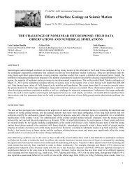
A NEW STRATEGY FOR DEVELOPING VS30 MAPS
David J. Wald Leslie McWhirter Eric Thompson Amanda S. Hering
U.S. Geological Survey Colorado School of Mines Tufts University Colorado School of Mines
Golden, CO 80401 Golden, CO 80401 Medford, MA 02155 Golden, CO 80401
USA USA USA USA
ABSTRACT
Despite obvious limitations as a proxy for site amplification, the use of time-averaged shear-wave velocity over the top 30
m (Vs 30 ) is useful and widely practiced, most notably through its use as an explanatory variable in ground motion
prediction equations (and thus hazard maps and ShakeMaps, among other applications). Local, regional, and global Vs 30
maps thus have diverse and fundamental uses in earthquake and engineering seismology. As such, we are developing an
improved strategy for producing Vs 30 maps given the common observational constraints available in any region for various
spatial scales. We investigate a hierarchical approach to mapping Vs 30 , where the baseline model is derived from
topographic slope because it is available globally, but geological maps and Vs 30 observations contribute, where available.
Using the abundant measured Vs 30 values in Taiwan as an example, we analyze Vs 30 versus slope per geologic unit and
observe minor trends that indicate potential interaction of geologic and slope terms. We then regress Vs 30 for the geologic
Vs 30 medians, topographic-slope, and cross-term coefficients for a hybrid model. The residuals of this hybrid model still
exhibit a strong spatial correlation structure, so we use the kriging-with-a-trend method (the trend is the hybrid model) to
further refine the Vs 30 map so as to honor the Vs 30 observations. Unlike the geology or slope models alone, this strategy
takes advantage of the predictive capabilities of the two models, yet effectively defaults to ordinary kriging in the vicinity
of the observed data, thereby achieving consistency with the observed data.
Keywords: Vs30, topographic slope, geology, kriging, site amplification condition

INTRODUCTION
Recognition of the importance of the ground-motion amplification from regolith has led to the development of systematic approaches
to quantifying both amplitude- and frequency-dependent site amplification (e.g., Borcherdt, 1994), as well as schemes for regionally
mapping seismic site conditions (e.g., Park and Elrick, 1998; Wills et al., 2000; Holzer et al., 2005). Measuring or mapping Vs 30 was
and is still a standard approach for mapping seismic site conditions. In fact, many U.S. building codes require site characterization
explicitly as Vs 30 (e.g., Dobry et al., 2000; Building Seismic Safety Council, BSSC, 2000). In addition, many of the modern groundmotion
prediction equations (e.g., Boore and Atkinson, 2008; Chiou and Youngs, 2008) are explicitly calibrated against seismicstation
site conditions described with Vs 30 values, and these in turn are employed in probabilistic (Kalkan et al., 2010) as well as realtime
hazard assessments, as in ShakeMap (e.g., Wald et al., 1999). The use of Vs 30 as a proxy for site amplification is widespread and
important in a number of hazard and risk-related endeavors.
Yet, there is no question that the use of Vs 30 as a proxy for site amplification has significant limitations, especially its lack of
information pertaining to frequency dependence, and its inability to distinguish between the response of velocity gradients and sharp
contrasts for which the Vs 30 may be similar. Castellaro et al. (2008), among others, suggested a litany of other limitations in using
Vs 30 as a proxy for site amplification. Notwithstanding its limitations, which we readily acknowledge, a number of important
applications, including hazard and risk maps, and ShakeMaps, will continue the use of Vs 30 given the current lack of systematically
available and readily employable alternatives.
An advantage of the use of Vs 30 measurements rather than more complex site amplification characterizations (e.g., frequencydependent
empirical measurements, or H/V ratios; Lermo and Chávez-García, 1993)—and perhaps one of the reasons it is so widely
in use—is the ability to extrapolate Vs 30 point observations to maps and thus to apply the very limited existing data to important
regional hazard mapping applications. It is exactly this advantage—the ability to map a proxy for site amplification over wide areas—
upon which we expand in this study.
We first describe existing Vs 30 mapping strategies. Two of these approaches, using geology- and topographic-slope-based proxies, are
attractive in that both are available in many areas of the world and can thus be applied over wide regions. However, as described next,
both have limitations as they are currently employed. As a proposed alternative, in areas where numerous Vs 30 observations have been
made, we can utilize them explicitly, both for improving the geology- and slope-based relationships to Vs 30 , as well as with
geostatistical analyses to incorporate the observations directly (kriging with a trend). We use an example from Taiwan to describe this
revised strategy for Vs 30 mapping. Finally, we generalize this approach, outlining an overall “recipe” for hierarchical Vs 30 mapmaking,
dependent on the available data sources in a particular region and based on the tools described herein. This new mapping
strategy provides motivation for collecting Vs 30 data at any spatial scale, since any new data can be used explicitly in refining Vs 30
maps: geostatistically, both local point constraints and regional trend removal can be used to reconcile Vs 30 data on different spatial
scales. In turn, these new data sets and the mapping algorithms described will be built into a refined version of the U.S. Geological
Survey’s Global Vs 30 Server (http://earthquake.usgs.gov/vs30/).
EXISTING VS30 MAP STRATEGIES
Several methodologies exist for extending the utility of spatially limited Vs 30 observations to larger areas. On the largest-scale maps,
for instance, for microzonation, densely sampled Vs 30 measurements can simply be spatially interpolated to cover limited regions rich
in data. For example, Hunter et al. (2010) developed a Vs 30 map (NEHRP site classes A through E) for the city of Ottawa, Canada by
kriging over 600 Vs 30 points, extracted from multiple geophysical sampling techniques. Effectively, the abundant data were simply
contoured, though where data points were less-densely sampled, consideration of known surficial geological boundaries was used in
the final contouring. The resulting Vs 30 map was used for the Ottawa Urban Earthquake Hazard Mapping program. Rarely are such
comprehensive Vs 30 data sets available. More usually, even in well-studied urban areas with high seismic risks, numbers of Vs 30
measurements reach only into the hundreds and more often the dozens; most urban areas have few openly available Vs 30 data sets.
Maps of seismic site conditions on more regional scales are not always available because they require substantial investment in
geological and geotechnical data acquisition as well as interpretation. For extending limited observations to smaller-scale maps,
several strategies are in use. A standard strategy, referred to here as “geology-based”, relies on the premise that mapped near-surface
geologic units can be reliable indicators of Vs 30 values within that unit wherever it has been mapped (e.g., Fumal and Tinsley, 1985;
Park and Ellrick, 1998; Wills et al., 2000). Surficial geological units are assigned a constant Vs 30 value usually based either on the
median value of Vs 30 of all observations inclusive to that unit (e.g., Fumal and Tinsley, 1985; Park and Elrick, 1998; Wills and Silva,
1998; Wills et al., 2000, Wills and Clahan, 2006); or, commonly, they are assigned via expert opinion based on Vs 30 values indicative
of these likely values within the geological units based on representative Vs 30 values.
2

The geology-based strategy can provide very useful Vs 30 maps in some cases (e.g., Wills and Clahan, 2006; Wills and Gutirrez, 2008).
Yet, there remains a substantial amount of subjectivity in turning the (often) large number of geological units into the sufficiently few
groupings needed for numerically assigning median Vs 30 values to each; there are insufficient Vs 30 data to constrain all individual
units. Since some or many of the units within the groups have not been sampled by Vs 30 measurements, the uncertainty of the Vs 30
values are not accounted for and are, in fact, solely dependent on subjective geological inferences. Furthermore, grouping geological
units and assigning a Vs 30 value to each grouping results in a constant value over large areas of the map (e.g., Fig. 1c, after Lee et al.,
2001), even though the Vs 30 observations show much greater, often systematic, spatial variations within those groups (e.g., compare
Fig. 1b and 1c). Worse, in many seismically active regions of the world, information about surficial geology and Vs 30 either does not
exist, varies dramatically in resolution and quality, varies spatially, or is not available in digital form.
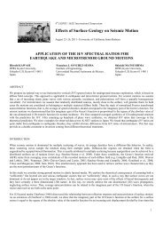
Fig. 1. A) Left: Topographic map of Taiwan at 30 arcsec (~1 km) sampling from STRM data; see legend for elevations. Circles
denote Vs 30 observations (downhole measurements from Lee et al., 2001); color fill is Vs 30 values (m/sec) as given by NEHRP
categories shown in the Vs 30 legend. B) Middle: Map of Vs 30 values predicted from the Wald and Allen (2007) model relating
topographic-slope to Vs 30 . C) Right: Geologic-based Vs 30 map of Lee et al. (2001); note Lee et al. (2001) use only four discrete
categorical geology units.
Topographic elevation data, on the other hand, are available at uniform sampling for the globe (e.g., SRTM data, Farr and Kobrick,
2000). Recognizing the global availability of high-resolution topographic data, Wald and Allen (2007) proposed an alternative
approach to systematically estimating and thus mapping Vs 30 using topographic slope as a predictor of Vs 30 . By taking the gradient of
the topography and choosing ranges of slope that maximize the correlation with shallow shear-velocity observations, they could
recover, to first order, many of the spatially varying features of site-condition maps developed for tectonically-active regions like
Taiwan and California, as well as for the low-relief, stable-craton regions like the Mississippi Embayment. Notably, the topographicslope
approach also predicted the bulk of the Vs 30 observations in these regions despite being derived for much wider data sets (Wald
and Allen, 2007; Allen and Wald, 2009). Unlike the geology-based approach, the slope-based strategy predicts Vs 30 values that
preserve the character of the observed spatial variations (e.g., compare the Vs 30 observations in Fig. 1a with Fig. 1b). Subsequent
analyses of the topographic-slope proxy for Vs 30 have shown convincing results (e.g., Wills and Gutierrez, 2008; Thompson et al.,
2011) in particular regions, though slope alone was certainly not expected to work well under all geological or geomorphic domains
(Wald and Allen, 2007).
Intuitively, topographic variations should be an indicator of near-surface geomorphology and lithology to the first order, with steep
mountains indicating rock, nearly flat basins indicating soil, and a transition between the end members on intermediate slopes. Slope
of topography, or gradient, should be diagnostic of Vs 30 , because more competent (high-velocity) materials are more likely to maintain
a steep slope whereas deep basin sediments are deposited primarily in environments with very low gradients. Furthermore, particle
size or sediment fineness, itself a predictor of lower Vs (e.g., Park and Elrick, 1998), should relate to slope. For example, steep, coarse,
mountain-front alluvial fan material typically grades to finer deposits with distance from the mountain front as is deposited at
decreasing slopes by less energetic fluvial and ultimately pluvial processes.
3

When detailed geomorphic, geologic, and geospatial data are systematically available, additional and very logical predictor variables
can improve the prediction of measured Vs 30 values. Matsuoka et al. (2005) found impressive correlations with Vs 30 in Japan among
slope, surficial geology, and combinations of geomorphic indicators (for example, man-made fill versus natural fill, distance to
mountain front, depositional environment, and elevation). However, outside of Japan, such detailed geomorphic indicators are not
widely mapped and are thus not digitally available.
After recognizing the correlation of slope with Vs 30 within particular quaternary soils units, Wills and Gutierrez (2008) suggested
employing slope as a corrective factor over uniform Vs 30 assignments within basin geological units. This combination of geology and
slope was investigated but was not ultimately employed in the map made available for distribution from their study; their revised map
employed refined geologic divisions but not the Vs 30 gradients within those units that slope would suggest.
Yong et al. (2008) employed semi-automated digital imaging analyses of Advanced Space-borne Thermal Emission and Reflection
Radiometer (ASTER) satellite imagery, combined with topography based on the same SRTM (30 arc-second sampling) data used by
Wald and Allen (2007), to break up topographic variations (e.g., slope, convexity, and roughness) into assignments to terrain units
(e.g., mountain, piedmont, and basin). These terrain units were then assigned Vs 30 ranges by average observations within those units.
However, many of the units were poorly sampled by Vs 30 data, and the lack of diverse lower-velocity units limit resolution at low Vs 30
(high amplification). As their approach relied only on remotely-sensed data, it too can potentially be applied globally. However, it is
unclear how the terrain unit assignments are independent of the slope and geologic-based predictor variables used in earlier studies.
One limiting aspect of all these state-of-the-art strategies for generating estimated Vs 30 maps, whether from geologic (e.g., Wills et al.,
2000; Wills and Clahan, 2006) or topographic base maps (e.g., Wald and Allen, 2007; Allen and Wald, 2009), or terrain (Matsuoka et
al., 2005; Yong et al., 2008) predictors is that, while initially derived from or constrained by observed Vs 30 values, these approaches
fail to directly incorporate the Vs 30 measurements used back into the map that has been created. Likewise, there are no strategies in
place for accommodating clear regional trends that obviously deviate from a priori slope or geology trend models, especially when
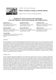
significant, new Vs 30 data become available. For example, Fig. 2 shows a comparison of logarithmic trends of topographic slope
versus measured Vs 30 for Taiwan (black) and for the Salt Lake City, Utah region (red). Regional trends in the relationship between
Vs 30 and slope may be significant, and perhaps related to the nature of the geologic units, and controlled by variations in depositional
and active tectonic environments. Moving forward, we have developed a strategy to not only directly incorporate all available Vs 30
into the mapping process, but to also let these data inform the recalibration, removing any regional trends in Vs 30 versus slope as well
as geology.
A REVISED VS30 MAPPING STRATEGY
For combining Vs 30 data directly into a joint model of Vs 30 (i.e., topographic slope-based or geology-based) we will employ the
geostatistical strategy of kriging. What makes kriging special is that it accounts for the spatial dependence among observations.
Kriging allows us to estimate Vs 30 at unsampled locations from the observed values; kriging itself is a generalized least-squares
regression algorithm. Any sufficiently well-sampled Vs 30 data can also be used to refine our a-priori predictive models, so rather than
ordinary kriging, we can employ kriging with a trend (KT; for more background see, for example, Thompson et al., 2010). Simple
kriging (SK) assumes that the trend is known and constant, ordinary kriging (OK) assumes it is unknown but still constant, and kriging
with a trend (KT), also known as “universal kriging,” allows the trend to fluctuate in space (Goovaerts, 1999). The geostatistical
literature often employs many different terms for what are rather similar techniques. Universal kriging, kriging with external drift, and
regression-kriging are basically the same.
The two potential trends we explore, topographic slope and geology, will be modified by inverting for the best-fit coefficients for
slope and mean Vs 30 per geologic unit. Here we take advantage of the notion that the drift and residuals can be estimated separately
and then summed (e.g., Thompson et al., 2010). These revised trends will be removed from the data, and since the residuals of this
hybrid model exhibit a strong spatial correlation structure, we will use the kriging with a trend method (the trend is the hybrid model)
to further refine the Vs 30 model-based map with the observed Vs 30 values. In a sense, we are modeling both the deterministic (trend)
and stochastic (variability) components of spatial Vs 30 variations separately. Unlike the geology or slope models alone, this strategy
takes advantage of the predictive capabilities of the both the geology and slope models, and potentially their interaction, yet
effectively defaults to ordinary kriging in the vicinity of the observed data, thereby achieving consistency with the observed data.
4

10 3
Utah
Taiwan
log [Shear Velocity (Vs30)]
10 2
0.001 0.01 0.1 1
log [Slope of Topography]
Fig. 2. Comparison of measured Vs 30 (m/sec) versus topographic slope (m/m) for Taiwan (black) and the Salt
Lake City, Utah region (red). The lines represent least-squares fits separately for the Taiwan and Salt Lake City
data. The linear fits have similar slopes, but the fit for the Taiwan data is vertically shifted from the fit for the Salt
Lake City data. This consistent difference between predicted Vs30 values for Taiwan and Salt Lake City may be
explained by the varied depositional and active orogenic environments.
MODELING AND RESULTS
Determining the optimal coefficients for slope, mean geological Vs 30 values, and any interactions (cross-terms) can be solved using
ordinary least squares (OLS) or, more optimally, using Generalized Least Squares (GLS). Ideally, any remaining correlation in the
covariance function of the residuals from OLS would be used iteratively to obtain the GLS coefficients, but such a strategy is unlikely
to be warranted given the limited amount and quality of the typical Vs 30 data set. GLS could be explored with a more comprehensive
Vs 30 data set than what is available for Taiwan (perhaps the Vs 30 data for the city of Ottawa, Canada; e.g., Hunter et al., 2010).
The primary variable of interest is Vs 30, which we assume to be log-normally distributed. If we let y = log 10 (Vs 30 ), for example, given
four geologic units, we can express the OLS model as:
! ! ! ! ! ! !! ! ! ! ! !! ! ! ! ! !! ! ! ! !!!! ! ! ! ! !! ! ! ! ! ! ! !! ! ! ! ! ! ! !! ! ! ! ! ! ! ! (1)
Here, ! ! , ! ! , and ! ! are indicator variables for the geologic units, ! ! denotes the topographic slope, ! ! , ! ! , and ! ! are factors
adjusting the intercept of the baseline geology units, and ! ! , ! ! , and ! ! are adjustments to the slope within the same units, ! !
represents the combined slope and geology intercept, and ! is a residual term. In general, any interaction terms, say ! ! , could be
insignificant if the relationships between slope and observed Vs 30 for units ! ! ! ! are similar, and could be dropped. Likewise, fewer or
more than four geological units could be easily represented and corresponding coefficients could be determined.
If it is deemed that interaction terms are unnecessary, or the coefficients cannot be constrained, we drop those terms:
! ! ! ! ! ! !! ! ! ! ! !! ! ! ! ! !! ! ! ! !!!! ! ! ! ! !! (2)
5

Conversely, where individual geological classes are not well sampled, only modifications to the general slope terms are afforded, and
the resulting map will default to the slope model, modified with the model residuals (Vs 30 data) as described below. Likewise, in
regions were geologic maps are either inadequate or are not digitally available, we let ! ! ! ! ! =!! ! ! !!!so any local Vs 30 data can be
used for solving for only the baseline and slope terms of the topographic-slope model:
! ! ! ! ! ! !! ! ! ! ! ! (3)
Any remaining spatially-correlated residuals in the data from that trend can be kriged as described below. First, determining whether
or not cross-terms (allowing variations of slope coefficients within each geologic unit) are needed must be explored by examining
whether or not slope trends can be found to exist (and differ) among and within individual geological units. If cross terms are
unneeded, a single slope coefficient is sufficient among the geological categories explored, or that there are insufficient data to justify
variable slopes per unit.
Regional variations in the relationship between slope and Vs30 were noted by Wald and Allen (2007); they found obvious differences
in slope-Vs 30 correlations between regions with active tectonics versus stable shields. Allen and Wald (2007) also noticed more subtle
variations within tectonically active areas, though the limited Vs 30 data limited resolution of these differences in all but the best data
sets. Given the likely dependence of slope versus Vs 30 on a variety of geologic sources and processes, perhaps it is not surprising to
find such differences, yet lacking an understanding of the dominant physical mechanisms controlling these relationships, we should
use care when interpreting them. However, in Fig. 2, there is clearly a distinguishable offset in the slope-Vs 30 relationship between
Taiwan and Utah; such differences require different trends among different regions. Next, we explore if such trend differences are
significant and distinguishable among different geologic units within our region of interest.
.+/0/12#!#
%&'"#()*&+,-#
!"""#
!""#
"$"""!# "$""!# "$"!# "$!# !#
Topographic Slope
.+/0/12#3#
.+/0/12#'#
.+/0/12#4#
5/6+7#(.+/0/12#!-#
5/6+7#(.+/0/12#3-#
5/6+7#(.+/0/12#'-#
5/6+7#(.+/0/12#4-#
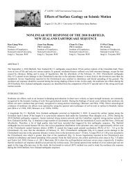
Fig. 3. Comparison of slope (m/m) and Vs 30 for Taiwan separated by geologic units. Color-coding for geological
units is similar to those shown in Fig. 1b. Lines are individual linear regressions for the Vs 30 for each unit.
In Fig. 3, we separate the Taiwan Vs 30 observations versus topographic slope by geologic unit to make exploratory scatter plots to see
if slope trends vary among the units. Separate Vs 30 versus slope trends among the geologic units would justify cross-terms, allowing
the mean geology and slope within a unit to behave independently of other units. We can then jointly regress Vs 30 from the geologic
classifications and the topographic-slope to derive coefficients for Vs 30 versus slope, the median geologic Vs 30 value, and offset as well
as cross terms. As seen in Fig. 3, some units have data with limited ranges of slope making comparison risky, yet the similarity in
trends does not strongly support the use of cross terms for a differing slope term within each geologic unit in this case. Thus, in the
current analysis, we limit our regression to equation (2).
Next, we need to process Vs 30 data points, gridded topographic data, and polygonal, categorical geological data. In practice, the grid
calculations and map-making are done using GMT (Wessel and Smith, 1995), and our kriging and regressions are done in R (R
Development Core Team, 2010). A flowchart of the procedure is provided in Fig. 4. In GMT, we compute the maximum slope from
the topography (Fig. 1a) as outlined by Wald and Allen (2007). The geological units (Fig. 1c), initially GIS shapefiles, are then
6

sampled at the same 30 arc-second sampling grid sampling as the topographic slope. The values of slope and geology category are
determined at each Vs 30 observation location. Then using R, we regress the equation (2) using ordinary least squares to determine the
coefficients, which are passed back to GMT.
Validation (Point)
Vs30 Data Set
Interpolation
(Point)
Vs30 Data Set
Continuous Predictor:
Topography
(Gridded) Data
Categorical
Predictor: Geology
(Polygon) Data
resample
resample
find slope at
Vs30 sites
geology at
Vs30 sites
Topographic
Slope
(Gridded)
Cross-term
analysis
Geology Grid
(indicator
variables)
fit remaining
trend
Fit
Coefficients
(Ordinary
Least
Squares)
Regression
Residuals
Trend
Estimates
Analyze residuals
for spatial correlation
(model variogram for
kriging)
Interpolate
Residuals
(Ordinary
Kriging)
Add interpolated
residuals
to fitted trend
Derive
Prediction Error
Evaluate
Accuracy
of
Estimates
Final Prediction
Vs30 Map
Vs30 Uncertainty
Map
Fig. 4. Flow chart for data processing, data analysis, regression modeling, and kriging. GMT processes are shown in
green; R functions in blue; white ovals are input data sets. Validation, refitting, and prediction error calculations (dashed
lines) have not yet been attempted. See text for details.
The forward calculation, estimating Vs 30 at all grid points, is done efficiently with GMT’s grid math processing and the results are
mapped in Fig. 5b. Next, residuals of the Vs 30 data from the forward model are determined at each observation point. Back in R (Fig.
3), kriging preprocessing involves generating and fitting a variogram (usually an exponential function) and determination of
appropriate sill, nugget, and range values (Fig. 6). The residuals are then kriged using these data-specific spatial correlation values,
and the results are resampled on the same uniform grid, which can be mapped back in GMT (Fig. 5c). Finally, the gridded, kriged
residuals are summed directly with the joint slope and geologic trend model to form the final Vs 30 map (Fig. 5d).
7

Lee et al [2001] and Wald and Allen [2007] Vs Model
Topography
Modelbased Vs30
24˚
24˚
22˚
22˚
120˚
122˚
120˚
122˚
Vs30 Observed Minus Model
Model + Residual
24˚
24˚
22˚
300200100 0 100 200 300
22˚
120˚
122˚
120˚
122˚
Fig. 5. a) Upper left: Topographic map and Vs 30 data for Taiwan; see Fig. 1 for details and legend. Black line shows the profile of
observations shown in Fig. 7; b) Upper right: map of Vs 30 trend model estimated with the combined slope and geology-based relations
derived by regression. c) Lower left: kriged residuals of Vs 30 observations (a) minus the trend model (b); see legend for residual values
(m/sec). d) Lower right: Final map generated by adding the kriged residuals (c) back onto the slope-based model (b)
8

From analysis of Fig. 5, we can see the desired contributions of the individual model components: the eastward gradient of Vs 30 from
along west coast of Taiwan in the combined trend model (Fig. 5b), and within a single geologic unit (see Fig. 1c), indicates the slopebased
contribution; the plume-shaped, southernmost NEHRP E-category geologic unit (Fig. 1c; near 120.3E, 22.3N) in the combined
trend model indicates some degree of geologic control; and, the modification of the trend model by the data as seen in Fig. 4d, clearly
indicates the role of individual Vs 30 data on the final model, for example, at and around the slowest Vs 30 sites in valleys and along the
west coast, or in the lowering of final Vs 30 values in the mountains in the north-central portion of the island.
The final combined trend model Fig. 5b more closely resembles the original (Fig.1b; Wald and Allen (2007) slope-based model than
the geologic-based model (Fig. 1c), though the slope model overestimated Vs 30 at some northern basin sites. In case of Taiwan, the
slope-model dominance is attributed to the favorable initial agreement of the Wald and Allen model with the observed Vs 30 and the
clear trends of Vs 30 within the separate, homogenous geologic units. It remains to be seen if this slope-model dominance will be the
norm in other tectonic or geomorphic environments. Clearly, however, the final Vs 30 map (Fig. 5d) is an improvement over the Wald
and Allen (2007) slope-based model in that it more closely matches observations at individual Vs 30 sites (Fig. 5a). A profile across
Taiwan (black line in Fig. 5a) is provided in Fig. 7, comparing Vs 30 values along section for the trend model (dashed line) and for the
final model with the kriged residuals added back in (Fig. 5d).
DISCUSSION
Although the procedure outlined here has only been applied, in this case, to one region, in essence we are proposing a simple “recipe”
for developing Vs 30 maps which should be generally applicable to any region of the world. In the absence of any Vs 30 data, or geologic
maps, the default becomes a slope-based Vs 30 map using predetermined Vs 30 –slope correlations determined for a comparable tectonic
environment elsewhere. With the addition of sufficient Vs 30 data (say, a few dozen values), the slope-Vs 30 correlation can be refined,
improving on a default trend, regressing for only the slope (of topographic slope versus Vs 30 ) and intercept coefficients (equation 2). If
geological maps are available, determine if cross-terms are needed, and adjust the use of equation (1) adding cross-terms accordingly.
The complete strategy for regression-kriging is then performed as described above, shown graphically in the flowchart in Figure 5, is
outlined here:
1) Assemble data sets:
a. Point Vs 30 data and uncertainties (down-hole, SASW, ReMi, CPT, etc.)
b. Assess the quality of the point data, assigning weights to reflect the quality of the measurements if necessary.
c. Digital topography: resolution 30 or 9 arc-second sampling (1 km or 250 m, respectively)
d. Digital geology maps (or, potentially, other Vs 30 -proxy maps); convert polygons to grids
2) Data preprocessing:
a. Topography:
i. Compute maximum slope values on grid.
ii. Sample slope at Vs 30 observation points.
b. Geology-based Vs 30 assignments:
i. Assign categorical (ordinal) values to geology map units.
ii. Sample geology units at Vs 30 data points.
3) Solve for combined slope and geology trend model coefficients. Generate forward model.
4) Compute residuals from the observed Vs 30 values minus the trend model.
5) Analyze Vs 30 residuals (variogram estimation; determine nugget, sill, and range).
6) Krige Vs 30 residuals and generate a grid of kriged residuals.
7) Add gridded kriged Vs 30 residuals back to trend model estimates.
8) Uncertainty analyses: compute cross-validation of data, map uncertainties.
Ongoing improvements in developing an optimal strategy for Vs 30 map development, include: i) the use of higher-resolution
topography (9 rather than 30 arc-second), ii) Employing sufficiency criteria (p-value) for employing topographic slope and geology
cross terms (equation 1), and iii) determination of estimated Vs 30 uncertainties. Allen and Wald (2009) and Wills and Gutirrez (2008)
have identified some limitations to higher resolution data, yet we anticipate that switching to 9 arc-second sampling (250-m spacing)
topographic data and re-deriving slope coefficients will be beneficial.
A final consideration is refining the Perl, R, and GMT scripts employed for semi-automating the production of Vs 30 maps in other
regions. Manual intervention will still be required for inspecting the variogram model (autocovariance function) needed for kriging
9

esiduals from the trend model. More significant work will be involved for areas in aggregating geological units appropriately and
commensurate with the Vs 30 data available to constrain their averages. A fundamental limitation of the geologic-based approach is the
trade-off between improved resolution and finer spatial variations offered by allowing more numerous geologic categories versus the
need to sample each with sufficient Vs 30 observations to constrain its median value.
The next task will be applying our strategy to Vs 30 data from glaciated terrains in New England and the upper Midwest (not tested by
Wald and Allen, 2007, using topographic slope alone), and then apply the “recipe” described above to develop a more refined Vs 30
map of the United States. In turn, that final product will replace the Vs 30 map now served by the USGS by their Global Vs30 Server
(http://earthquake.usgs.gov/vs30/).
Semivariance
50000
40000
30000
20000
10000
!
!
!
! !
!
! Empirical
Model
!
!
! ! !
!
!
!
!
!
!
!
!
! ! !! !
!
!
!
!
!
!
!
!
!
! !
! !
!
!
!
!
!
!!
!
! ! !
!
!
!
!
! !!
!
!
!!
!
!
!
!
0
0.0 0.5 1.0 1.5 2.0 2.5 3.0
Distance, deg
!
#
Fig. 6. Spatial correlation variogram for Vs 30 residuals from the combined model (Fig. 5b). Kriged residuals (5b)
employ a 5000 nugget, 25000 sill, and range (cutoff distance) of 0.5 degrees.
CONCLUSIONS
One limiting aspect of current state-of-the-art strategies for generating estimated Vs 30 maps, whether from geologic, topographic, or
remotely sensed base maps, is that although derived from or aimed to be consistent with observed Vs 30 values, these approaches fail to
directly incorporate the Vs 30 observations back into the map that has been created. Likewise, there are no strategies in place for
accommodating significant new Vs 30 data as they become available or where regional trends obviously deviate from the default trend
models.
The strategy described herein uses a hierarchical approach to mapping Vs 30 , taking full advantage of these most commonly available
data sources: topographic slope, surficial geological maps, and Vs 30 measurements. The baseline model is derived from topographic
slope because it is available globally, but geological maps and Vs 30 observations contribute where data are available. We analyze Vs 30
versus slope per geologic unit and observe minor trends that indicate some interaction of geologic and slope domains, but in the case
of Taiwan, not enough to warrant separate regression terms. We then regress Vs30 for the geologic Vs 30 medians and regional
topographic slope-Vs 30 coefficients for a hybrid topographic-slope/geologic model. The residuals of this hybrid model still exhibit a
strong spatial-correlation structure, so we use the kriging-with-a-trend method (the trend is the hybrid model) to insure we fit all Vs 30
observations at those sites. Unlike the geology or slope models alone, this strategy takes advantage of the predictive capabilities of the
10

two models, yet effectively defaults to ordinary kriging in the vicinity of the observed data, thereby achieving consistency with the
observed data.
Fig. 7. SW-NE profile (see track line on Fig. 5a) showing Vs 30 data (circles), and sampling the trend model (dashed,
Fig. 5b) and final kriged model (solid line, Fig. 5d). Wald and Allen’s (2007) topographic slope-based model (red
line) and Lee et al’s geology-based model (blue line) are also shown for comparison
ACKNOWLEDGEMENTS
Internal USGS reviews by Bruce Worden and Anna Olsen are greatly appreciated; Bruce also provided needed guidance on GMT’s
grdmath computations.
REFERENCES
Allen, T. I. and D. J. Wald [2009]. On the Use of High-Resolution Topographic Data as a Proxy for Seismic Site Conditions (VS 30 ),
Bull. Seism. Soc. Am., 99, No. 2A, pp. 935–943.
Allen, T. I. and D. J. Wald [2007]. Topographic Slope as a Proxy for Seismic Site Conditions (VS30) and Amplification around the
Globe, U.S.G.S. Open File Report 2007-1357, 69 pp.
Boore, D. M., and G. M. Atkinson [2008]. Ground-Motion Prediction Equations for the Average Horizontal Component of PGA,
PGV, and 5%-Damped PSA at Spectral Periods between 0.01 s and 10.0 s. Earthquake Spectra, 24(1), 99-138.
Boore, D.M., Asten, M.W. [2008]. Comparisons of shear-wave slowness in the Santa Clara Valley, California, from blind
interpretations of data from a comprehensive set of invasive and non-invasive methods using active- and passive-sources. Bull.
Seism. Soc. Am., 98, 1982–2003.
Borcherdt, R. D. [1994]. Estimates of site-dependent response spectra for design (methodology and justification), Earthquake Spectra,
10, 617-653.
Building Seismic Safety Council (BSSC) [2000]. National Earthquake Hazards Reduction Program (NEHRP) Part 1: Recommended
provisions for seismic regulations for new buildings and other structures, Federal Emergency Management Agency.
Castellaro, S., F. Mulargia, P. Rossi [2008]. Vs30: Proxy for site amplification, Seism. Res. Lett., 79, 540-544.
Chiou, B. S.-J., and R. R. Youngs [2008]. An NGA Model of the Average Horizontal Component of Peak Ground Motion and
Response Spectra. Earthquake Spectra, 24(1), 173-215.
11

Dobry, R., R. D. Borcherdt, C. B. Crouse, I. M. Idriss, W. B. Joyner, G. R. Martin, M. Power, E. Rinne, and R. B. Seed [2000]. New
site coefficients and site classification system used in recent Building Seismic Code provisions, Earthquake Spectra, 16, 41-67.
Farr, T. G., and M. Kobrick [2000]. Shuttle Radar Topography Mission produces a wealth of data, EOS Trans., 81, 583-585.
FEMA [1994]. NEHRP recommended provisions for the development of seismic regulations for new buildings, FEMA.
Fumal, T. E., and J. C. Tinsley [1985]. Mapping shear-wave velocities of near-surface geologic materials, Evaluating Earthquake
Hazards in the Los Angeles Region-An Earth-Science Perspective 1360, 101-126.
Goovaerts, P. [1999]. Geostatistics in soil science: state-of-the-art and perspectives, Geoderma, 89, 1–45.
Holzer, T. L., A. C. Padovani, M. J. Bennett, T. E. Noce, and J. C. Tinsley [2005]. Mapping Vs30 site classes, Earthquake Spectra,
21, 353-370.
Hunter, J A; Crow, H L; Brooks, G R; Pyne, M; Motazedian, D; Lamontagne, M; Pugin, A J -M; Pullan, S E; Cartwright, T; Douma,
M; Burns, R A; Good, R L; Kaheshi-Banab, K; Caron, R; Kolaj, M; Folahan, I; Dixon, L; Dion, K; Duxbury, A; Landriault, A;
Ter-Emmanuil, V; Jones, A; Plastow, G; Muir, D. [2010]. Seismic site classification and site period mapping in the Ottawa area
using geophysical methods, Geological Survey of Canada Open File 6273, 80 pages.
Kalkan, E., C. J. Wills, and D. M. Branum [2010]. Seismic Hazard Mapping of California Considering Site Effects, Earthquake
Spectra, 26, No. 4, pages 1039–1055.
Lee, C.-T., C.-T. Cheng, C.-W. Liao, and Y.-B. Tsai [2001]. Site classification of Taiwan free-field strong-motion stations, Bull.
Seism. Soc. Am., 91, 1283-1297.
Lermo, J., and F. J. Chávez-García [1993]. Site effect evaluation using spectral ratios with only one station, Bull. Seism. Soc. Am., 83,
no. 5, 1574–1594.
Matsuoka, M., K. Wakamatsu, K. Fujimoto, and S. Midorikawa [2005]. Nationwide site amplification zoning using GIS-based Japan
engineering geomorphologic classification map, Proc. 9th Inter. Conf. on Struct. Safety and Reliability, 239-246.
Park, S., and S. Elrick [1998]. Predictions of shear-wave velocities in southern California using surface geology, Bull. Seism. Soc.
Am., 88, 677-685.
R Development Core Team [2010]. R: A Language and Environment for Statistical Computing, R Foundation for Statistical
Computing, Vienna, Austria.
Thompson, E. M., L. G. Baise, R. E. Kayen, E.C. Morgan, and J. Kaklamanos [2011]. Multiscale Site-Response Mapping: A Case
Study of Parkfield, California, Bull. Seism. Soc. Am., 101, 1081–1100.
Thompson, E. M., L. G. Baise, R. E. Kayen, Y. Tanaka, and H. Tanaka [2010]. A geostatistical approach to mapping site response
spectral amplifications, Eng. Geol., 114, no. 3–4, 330–342.
USGS Global Vs30 Server [2011]. 30-arc-sec resolution global slope-based Vs30 proxy maps. http://earthquake. usgs.gov/vs30/.
Wald, D. J., P. S. Earle, and V. Quitoriano [2004]. Topographic Slope as a Proxy for Seismic Site Correction and Amplification, EOS.
Trans. AGU, 85(47), F1424.
Wald, D. J., and T. I. Allen [2007]. Topographic slope as a proxy for seismic site conditions and amplification, Bull. Seism. Soc. Am.,
97, No. 5, 1379-1395.
Wald, D. J., V. Quitoriano, T.H. Heaton, H. Kanamori, C.W. Scrivner and C.B. Worden [1999]. TriNet "ShakeMaps": Rapid
generation of peak ground motion and intensity maps for earthquakes in southern California, Earthquake Spectra, 15, 537-555.
Wessel, P., and W. H. F. Smith [1995]. New Version of the Generic Mapping Tools Released, EOS Trans. AGU, 76, 329.
Wills, C. J. and C. Gutierrez [2008]. Investigation of geographic rules for improving site-conditions mapping, Calif. Geo. Sur. Final
Tech. Rept., 20 pp. (Award No. 07HQGR0061).
Wills, C. J., and K. B. Clahan [2006]. Developing a map of geologically defined site-condition categories for California, Bull. Seism.
Soc. Am., 96, 1483–1501.
Wills, C. J., M. Petersen, W. A. Bryant, M. Reichle, G. J. Saucedo, S. Tan, G. Taylor, and J. Treiman [2000]. A site-conditions map
for California based on geology and shear-wave velocity, Bull. Seism. Soc. Am., 90, S187–S208.
Wills, C. J., and W. Silva [1998]. Shear-wave velocity characteristics of geologic units in California, Earthquake Spectra, 14, 533-
556.
Yong, A., Hough, S.E., Abrams, M.J., Cox, H.M., Wills, C.J., Simila, G.W. [2008]. Site characterization using integrated imaging
analysis methods on satellite data of the Islamabad, Pakistan, Region, Bull. Seism. Soc. Am. 98, 2679–2693.
12