a new strategy for developing vs30 maps - ESG4 Conference @ UCSB

Conversely, where individual geological classes are not well sampled, only modifications to the general slope terms are afforded, and
the resulting map will default to the slope model, modified with the model residuals (Vs 30 data) as described below. Likewise, in
regions were geologic maps are either inadequate or are not digitally available, we let ! ! ! ! ! =!! ! ! !!!so any local Vs 30 data can be
used for solving for only the baseline and slope terms of the topographic-slope model:
! ! ! ! ! ! !! ! ! ! ! ! (3)
Any remaining spatially-correlated residuals in the data from that trend can be kriged as described below. First, determining whether
or not cross-terms (allowing variations of slope coefficients within each geologic unit) are needed must be explored by examining
whether or not slope trends can be found to exist (and differ) among and within individual geological units. If cross terms are
unneeded, a single slope coefficient is sufficient among the geological categories explored, or that there are insufficient data to justify
variable slopes per unit.
Regional variations in the relationship between slope and Vs30 were noted by Wald and Allen (2007); they found obvious differences
in slope-Vs 30 correlations between regions with active tectonics versus stable shields. Allen and Wald (2007) also noticed more subtle
variations within tectonically active areas, though the limited Vs 30 data limited resolution of these differences in all but the best data
sets. Given the likely dependence of slope versus Vs 30 on a variety of geologic sources and processes, perhaps it is not surprising to
find such differences, yet lacking an understanding of the dominant physical mechanisms controlling these relationships, we should
use care when interpreting them. However, in Fig. 2, there is clearly a distinguishable offset in the slope-Vs 30 relationship between
Taiwan and Utah; such differences require different trends among different regions. Next, we explore if such trend differences are
significant and distinguishable among different geologic units within our region of interest.
.+/0/12#!#
%&'"#()*&+,-#
!"""#
!""#
"$"""!# "$""!# "$"!# "$!# !#
Topographic Slope
.+/0/12#3#
.+/0/12#'#
.+/0/12#4#
5/6+7#(.+/0/12#!-#
5/6+7#(.+/0/12#3-#
5/6+7#(.+/0/12#'-#
5/6+7#(.+/0/12#4-#
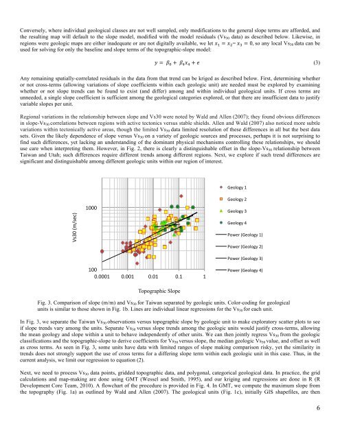
Fig. 3. Comparison of slope (m/m) and Vs 30 for Taiwan separated by geologic units. Color-coding for geological
units is similar to those shown in Fig. 1b. Lines are individual linear regressions for the Vs 30 for each unit.
In Fig. 3, we separate the Taiwan Vs 30 observations versus topographic slope by geologic unit to make exploratory scatter plots to see
if slope trends vary among the units. Separate Vs 30 versus slope trends among the geologic units would justify cross-terms, allowing
the mean geology and slope within a unit to behave independently of other units. We can then jointly regress Vs 30 from the geologic
classifications and the topographic-slope to derive coefficients for Vs 30 versus slope, the median geologic Vs 30 value, and offset as well
as cross terms. As seen in Fig. 3, some units have data with limited ranges of slope making comparison risky, yet the similarity in
trends does not strongly support the use of cross terms for a differing slope term within each geologic unit in this case. Thus, in the
current analysis, we limit our regression to equation (2).
Next, we need to process Vs 30 data points, gridded topographic data, and polygonal, categorical geological data. In practice, the grid
calculations and map-making are done using GMT (Wessel and Smith, 1995), and our kriging and regressions are done in R (R
Development Core Team, 2010). A flowchart of the procedure is provided in Fig. 4. In GMT, we compute the maximum slope from
the topography (Fig. 1a) as outlined by Wald and Allen (2007). The geological units (Fig. 1c), initially GIS shapefiles, are then
6