a new strategy for developing vs30 maps - ESG4 Conference @ UCSB
a new strategy for developing vs30 maps - ESG4 Conference @ UCSB
a new strategy for developing vs30 maps - ESG4 Conference @ UCSB

You also want an ePaper? Increase the reach of your titles
YUMPU automatically turns print PDFs into web optimized ePapers that Google loves.
10 3<br />
Utah<br />
Taiwan<br />
log [Shear Velocity (Vs30)]<br />
10 2<br />
0.001 0.01 0.1 1<br />
log [Slope of Topography]<br />
Fig. 2. Comparison of measured Vs 30 (m/sec) versus topographic slope (m/m) <strong>for</strong> Taiwan (black) and the Salt<br />
Lake City, Utah region (red). The lines represent least-squares fits separately <strong>for</strong> the Taiwan and Salt Lake City<br />
data. The linear fits have similar slopes, but the fit <strong>for</strong> the Taiwan data is vertically shifted from the fit <strong>for</strong> the Salt<br />
Lake City data. This consistent difference between predicted Vs30 values <strong>for</strong> Taiwan and Salt Lake City may be<br />
explained by the varied depositional and active orogenic environments.<br />
MODELING AND RESULTS<br />
Determining the optimal coefficients <strong>for</strong> slope, mean geological Vs 30 values, and any interactions (cross-terms) can be solved using<br />
ordinary least squares (OLS) or, more optimally, using Generalized Least Squares (GLS). Ideally, any remaining correlation in the<br />
covariance function of the residuals from OLS would be used iteratively to obtain the GLS coefficients, but such a <strong>strategy</strong> is unlikely<br />
to be warranted given the limited amount and quality of the typical Vs 30 data set. GLS could be explored with a more comprehensive<br />
Vs 30 data set than what is available <strong>for</strong> Taiwan (perhaps the Vs 30 data <strong>for</strong> the city of Ottawa, Canada; e.g., Hunter et al., 2010).<br />
The primary variable of interest is Vs 30, which we assume to be log-normally distributed. If we let y = log 10 (Vs 30 ), <strong>for</strong> example, given<br />
four geologic units, we can express the OLS model as:<br />
! ! ! ! ! ! !! ! ! ! ! !! ! ! ! ! !! ! ! ! !!!! ! ! ! ! !! ! ! ! ! ! ! !! ! ! ! ! ! ! !! ! ! ! ! ! ! ! (1)<br />
Here, ! ! , ! ! , and ! ! are indicator variables <strong>for</strong> the geologic units, ! ! denotes the topographic slope, ! ! , ! ! , and ! ! are factors<br />
adjusting the intercept of the baseline geology units, and ! ! , ! ! , and ! ! are adjustments to the slope within the same units, ! !<br />
represents the combined slope and geology intercept, and ! is a residual term. In general, any interaction terms, say ! ! , could be<br />
insignificant if the relationships between slope and observed Vs 30 <strong>for</strong> units ! ! ! ! are similar, and could be dropped. Likewise, fewer or<br />
more than four geological units could be easily represented and corresponding coefficients could be determined.<br />
If it is deemed that interaction terms are unnecessary, or the coefficients cannot be constrained, we drop those terms:<br />
! ! ! ! ! ! !! ! ! ! ! !! ! ! ! ! !! ! ! ! !!!! ! ! ! ! !! (2)<br />
5