Quantitative effects of composting state variables on ... - ResearchGate

More documents

Recommendations

Info

1246 W. Sun et al. / Science <strong>of</strong> the Total Environment 409 (2011) 1243–1254 3.2. Dataset All the observed data from the six runs <strong>of</strong> food waste <strong>composting</strong> were collected (198 samples) and combined to form the whole dataset. Each sample was a combination <strong>of</strong> inputs (i.e. <strong>state</strong> <strong>variables</strong> and SCA's inherent parameters) and the C/N ratio. The <strong>state</strong> <strong>variables</strong> had potential <strong>effects</strong> on C/N ratio variation; they included time (X 1 ), mean temperature (X 2 ), pH (X 3 ), moisture content (X 4 ), ash content (X 5 ), organic content (X 6 ), NH + 4 -N concentration (X 7 ), cumulative NH 3 emissions (X 8 ), log colony count <strong>of</strong> thermophilic bacteria (X 9 ), log colony count <strong>of</strong> mesophilic bacteria (X 10 ), upper temperature (X 11 ), and lower temperature (X 12 ). Although the sum <strong>of</strong> X 4 ,X 5 and X 6 was one, the three <strong>state</strong> <strong>variables</strong> were still included since it was difficult to exclude one <strong>of</strong> them from the candidates subjectively; The SCA's inherent parameters were α cut (significance level for cutting clusters), α merge (significance level for merging clusters), and N min (the minimum number <strong>of</strong> samples within tip clusters). The C/N ratio was the concerned output. The entire dataset was randomly divided into a training set (167 samples, 84%) and a test set (31 samples, 16%). The training set was used for calibrating the GASCA (or SCA) forecasting trees and the test one was for verification in independent samples from different reactors. Since the magnitudes <strong>of</strong> <strong>state</strong> <strong>variables</strong> were significantly different from each other, we firstly converted all input datasets into the range <strong>of</strong> [−1, 1] before the training process and then transformed the values <strong>of</strong> the predicted dependent <strong>variables</strong> back to their original ranges after the training was completed. 3.3. Principle <strong>of</strong> stepwise cluster analysis (SCA) SCA is based on the theory <strong>of</strong> multivariate analysis <strong>of</strong> variance. Generally, two phases are involved in its implementation: training and test. In the training phase, the sample dataset is cut into two subsets (clusters) and then two are merged into one during the iterative training process. According to Wilks' likelihood-ratio criterion, the cutting point is optimal only if the value <strong>of</strong> Wilks' Λ is minimum (Wilks, 1962). Since the Λ is directly related to the F statistic, the sample means <strong>of</strong> the two sub-clusters can be compared for significant differences through F test (Rao, 1952). Thus, the criteria <strong>of</strong> cutting (or merging or not) clusters rely on a set <strong>of</strong> F tests (Rao, 1965; Tatsuoka, 1971). Based on the F tests, a tree is shaped step by step until no subsets could be cut or merged any more. In the test phase, the values <strong>of</strong> the new independent <strong>variables</strong> in the test samples will be used as references to determine which child cluster a sample in the parent cluster will enter. Thus, the sample would gradually enter one tip cluster. The mean <strong>of</strong> dependent <strong>variables</strong> from the training set at the tip cluster that the sample finally enters becomes the predicted value <strong>of</strong> the sample's dependent variable. A more detailed description <strong>of</strong> SCA can be referred to our previous work (Qin et al., 2008). 3.4. Variable/parameter selection using GA An integrated GASCA model combining GA with SCA would possess abilities in both variable searching and nonlinear fitting. 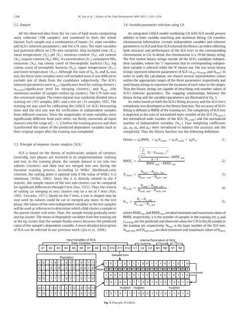GA transfers chromosome information (certain independent <strong>variables</strong> and inherent parameters) to SCA and then SCA returned the fitness (an index reflecting both structure and performance <strong>of</strong> the SCA tree) to the corresponding chromosome in GA. In detail, the chromosome is a 19-bit binary string. The first twelve binary strings encode all the SCA's candidate independent <strong>variables</strong>, where the ‘1’ represents that its corresponding independent variable is selected while the ‘0’ means not. The last seven binary strings represent inherent parameters <strong>of</strong> SCA (α cut , α merge and N min ). In order to unify the calculation, we chosen several representative values within the appropriate ranges <strong>of</strong> the three parameters respectively and used binary strings to represent the locations <strong>of</strong> each value in the ranges. Thus the binary strings are capable <strong>of</strong> describing real-number values <strong>of</strong> SCA's inherent parameters. The mapping relationships between the binary string and the <strong>variables</strong>/parameters are illustrated in Fig. 3. An index based on both the SCA's fitting accuracy and the SCA tree's complexity was developed as the fitness function. The accuracy <strong>of</strong> SCA's fitting is defined as RMSE <strong>of</strong> the training set. The complexity <strong>of</strong> SCA tree is depicted as the sum <strong>of</strong> normalized layer number <strong>of</strong> the SCA (N s,layer ), the normalized node number <strong>of</strong> the SCA (N s,node ) and the normalized number <strong>of</strong> independent <strong>variables</strong> (N s,x ). Four weighting coefficients (μ 1 , μ 2 , μ 3 , and μ 4 ) were introduced to balance the accuracy and the complexity. Thus the fitness function has the following definition: Fitness = μ 1 RMSE s + μ 2 N s;layer + μ 3 N s;node + μ 4 N s;x vffiffiffiffiffiffiffiffiffiffiffiffiffiffiffiffiffiffiffiffiffiffiffiffiffiffiffiffiffiffiffiffiffiffiffiffiffiffiffiffiffi n u∑ ðy j −y training; j Þ 2 tj =1 −RMSE n−1 min RMSE s = RMSE max −RMSE min N layer−N layer; min N s;layer = N layer; max −N layer; min N node−N node; min N s;node = N node; max −N node; min N s;x = N x−N x; min N x; max −N x; min where RMSE min and RMSE max are ideal minimum and maximum values <strong>of</strong> RMSE, respectively; n is the number <strong>of</strong> samples in the training set; y j and y training,j are the predicted and observed values for C/N in the jth sample in the training set, respectively; N layer is the layer number <strong>of</strong> the SCA tree. N layer,min and N layer,max are ideal minimum and maximum values <strong>of</strong> N layer , ð1Þ ð2Þ ð3Þ ð4Þ ð5Þ X1 Input Variables <strong>of</strong> SCA Internal Parameters <strong>of</strong> SCA State Variables α cut α merge N min X2 X3 X4 X5 X6 X7 X8 X9 X10 X11 X12 C1 C2 C3 M1 M2 N1 N2 Population 1 0 ... 1 0 1 ... 0 1 1 ... 0 1 1 1 1 1 ... 0 1 0 ... 0 1 0 ... 0 0 1 0 1 0 ... 1 1 1 ... 0 1 1 ... 0 1 1 0 0 0 ... 1 1 1 ... 0 1 1 ... 0 1 1 0 … … ... 0 1 ... 1 0 1 ... 0 1 0 ... 0 1 0 1 1 0 ... 1 0 1 ... 0 1 0 ... 0 1 1 0 Detailed form 1 0 1 1 0 1 1 1 0 0 1 1 1 0 1 1 0 1 0 Vector 1 1 1 0 1 0 1 0 1 0 1 0 1 0 1 0 1 0 1 1 0 0 0 1 1 0 1 1 0 1 0 0 0 1 0 1 1 0 1 0 1 0 0 1 1 1 0 0 1 0 1 0 1 0 0 1 0 mutation mutation mutation 1 0 1 0 1 1 1 0 0 0 1 0 1 0 1 1 0 1 0 crossover Fig. 3. Principle <strong>of</strong> GASCA.
W. Sun et al. / Science <strong>of</strong> the Total Environment 409 (2011) 1243–1254 1247 respectively; N node is the node number <strong>of</strong> the SCA tree; N node,min and N node,max are ideal minimum and maximum values <strong>of</strong> N node ,respectively; N x is the number <strong>of</strong> independent <strong>variables</strong>; N x,min and N x,max are ideal minimum and maximum values <strong>of</strong> N x , respectively. Similar to the construction <strong>of</strong> a single chromosome, a population with a group <strong>of</strong> chromosomes in GA would be randomly generated. Parents would be selected based on individuals' fitness values using the stochastic uniform method, then further intercrossed to exchange their genetic information by the scattered crossover method, and mutated through changing their information randomly by the Gaussian mutation method (The MathWorks, 2008). Generation by generation, parents with worse fitness would be replaced by children with better fitness in the evaluated population. Once the stopping criterion was satisfied; the chromosome with the lowest fitness value would represent the information <strong>of</strong> the final optimal combination <strong>of</strong> <strong>variables</strong>/parameters for SCA. 3.5. Program implementation <strong>of</strong> GASCA A flow diagram <strong>of</strong> GASCA is presented in Fig. 2. All programs were written in Matlab R2008a (The MathWorks, 2008). The main program for coupling GA and SCA is clarified as follows: Step 1: Before SCA training, the entire dataset (the <strong>state</strong> <strong>variables</strong> and C/N) is scaled to fall within the range <strong>of</strong> −1 to1; Step 2: A number (the default is 100) <strong>of</strong> randomly generated chromosomes (<strong>of</strong> a bit length equal to the number <strong>of</strong> <strong>state</strong> <strong>variables</strong> and inherent parameters chosen) form a population; Step 3: GA invokes the SCA function to evaluate fitness <strong>of</strong> every chromosome in the population: Step 4: New chromosomes are generated through selection, crossover, and mutation operations; GA invokes the SCA function to calculate fitness values <strong>of</strong> new chromosomes. Step 5: Replace the old chromosomes with new chromosomes; Step 6: After all operations, the chromosome with the worst fitness <strong>of</strong> the entire population is replaced with the current elitist; Step 7: Return to Step 4 to begin the evolution <strong>of</strong> the next generation; if the generation number exceeds a certain value (e.g. 25), the program will end. The computational procedures <strong>of</strong> the SCA function are described as follows: Step 1: GA will search the proxy table to find out whether the same chromosome is calculated already or not; if yes, the corresponding fitness will be assigned to the chromosome directly and the program goes to Step 12, and if no, goes to Step 2; Step 2: GA invokes SCA to evaluate the fitness <strong>of</strong> every chromosome: the entire training dataset will be cut into a smaller one based on the independent variable information embedded in the chromosome; such a dataset is treated as a leaf cluster (i.e. a cluster without sub-clusters); the parameter information (α cutting , α merging and N min ) will be used in Steps 9, 11 and 12; Step 3: For every leaf cluster, each <strong>state</strong> variable X id (i.e. independent <strong>variables</strong>, id=1, 2, …, m) is chosen in the order <strong>of</strong> X 1 to X m ; the samples (including both independent and dependent <strong>variables</strong>) in cluster σ (matrix) are sequenced to σ(X id )inan ascending order according to the value <strong>of</strong> X id ; Step 4: For the matrix σ(X id ), every cutting line nr (between row i to row i+1, nr=1, 2, …, n−1) is chosen in the order from 1 to n −1; n is the number <strong>of</strong> samples for cluster σ(X id ); the cluster σ(X id ) will be divided into two sub Clusters β and γ according to the cutting line; Step 5 The Wilks' Λ based on the dependent <strong>variables</strong> (Y β and Y γ )is calculated; by comparing all m*(n−1) values <strong>of</strong> Wilks' Λ, the minimal value <strong>of</strong> Λ(id*, nr*) can be obtained; Step 6: Calculate the F cal value; if F cal ≥F α-cuting , the parent cluster can be cut into two sub-clusters; Step 7: The independent variable and the value in the cutting point (x id *, nr*) becomes a judging criterion; all samples in this cluster with x id*, nr ≤x id*, nr* are allocated to one sub-cluster, with the rest to the other; Step 8: Repeat Steps 3 to 7 until all clusters are tested for possible cutting in the present layer; Step 9: When the cutting operation in the present layer is done, the merging operations begin; if other old leaf clusters exist, these new leaf clusters will be tested along with all other leaf clusters to demonstrate whether pairs <strong>of</strong> them could be merged into one cluster; the Wilks' Λ and F cal values will be calculated for each pair clusters; if F cal ≥F α-merging , the two clusters will be considered having no significant difference and can be merged; Step 10: If there are no other old leaf clusters or no merged operations are needed, the new leaf clusters will be treated as new clusters and tested for further cutting or merging operations according to Steps 3 to 9; Step 11: If no leaf cluster can be cut or merged or the number <strong>of</strong> samples in every cluster is less than N min , the training process is completed with the SCA tree being shaped; then, the fitness <strong>of</strong> chromosome is calculated based on Eqs. (1)–(5); Step 12: Return to Step 1 for evaluating the next chromosome; if the fitness <strong>of</strong> each existing chromosome has been evaluated, return to the main program. 4. Results 4.1. Structure <strong>of</strong> GA In general, GA's fitness function and operation (selection, crossover, and mutation) configurations have significant impacts on its performance. The fitness function is always problem-oriented; determination <strong>of</strong> its value (Eqs. (1)–(5)) depends on the relevant coefficients selection, according to the datasets <strong>of</strong> food waste <strong>composting</strong>. Through error and test, four weighting coefficients (i.e. μ 1 , μ 2 , μ 3 ,andμ 4 )forbalancingthe accuracy and the complexity <strong>of</strong> SCA were determined as 1.04, 0.35, 0.37 and 0.024. The coefficients for normalizing SCA' complexity calculation (i.e. RMSE min ,RMSE max ,N layer,min ,N layer,max ,N node,min, N node,max, N x,min and N x,max ) were configured as 0, 10, 3, 150, 3, 1500, 2 and 12, respectively. GA's standard operations are controlled by the relevant parameters, including the population size (PS), the selection rate (SR), the crossover fraction (CF, or crossover rate), and the mutation rate (MR). Usually, the larger the PS, the higher the CF; the higher the MR, the more diversified the chromosomes. However, a larger PS and a higher MR may lead to the requirement <strong>of</strong> more computational efforts. To obtain a relative optimal configuration <strong>of</strong> GA for supporting SCA's variable selection, PS and CF (MR=1–CF in our GA program) were chosen to examine their <strong>effects</strong> on fitness. We changed one <strong>of</strong> them in its possible range and kept the other at its default value during each observation. The results indicated that, when the PS increased from 20 to 110 by every 10 units, the obtained optimal fitness value would fluctuate and keep as a constant after the PS exceeds 100. Similarly, the obtained optimal fitness value would keep the same when CF was greater than 0.8 (in the range from 0 to 1 by every 0.05). Thus, the optimal setting <strong>of</strong> GA for SCA was set as: population size=100, crossover fraction=0.8 and maximum allowable generation=25. The operation processes <strong>of</strong> GA under such a setting are illustrated in Fig. 4. Over the entire GA iteration, the best,
Page 1 and 2: Science of the Tot
Page 3: W. Sun et al. / Science of<
Page 7 and 8: W. Sun et al. / Science of<

Quantitative effects of composting state variables on ... - ResearchGate

You also want an ePaper? Increase the reach of your titles

Delete template?

Save as template?