Quantitative effects of composting state variables on ... - ResearchGate

More documents

Recommendations

Info

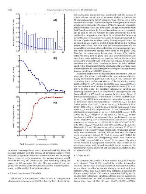
1248 W. Sun et al. / Science <strong>of</strong> the Total Environment 409 (2011) 1243–1254 Best, Worst, and Mean Scores Average Distance Times Calling Proxy Table 0.9 0.8 0.7 0.6 0.5 0.4 0.3 0.2 0.1 3.5 3 2.5 2 1.5 1 0.5 0 100 90 80 70 60 50 40 30 20 10 worse and the average fitness value (the vertical bars in Fig. 4a) would decrease gradually with the increase <strong>of</strong> generation number. There were always significant differences between the best and the average fitness values at each generation; the average distance would decrease instantly but automatically keep fluctuating during the process <strong>of</strong> GA operation (Fig. 4b). This demonstrated that the population diversity could be maintained and the undesired prematurity could be avoided during GA operations. 4.2. Interactions between SCA and GA 5 10 15 20 25 5 10 15 20 25 5 10 15 20 25 Generation (a) (b) (c) Fig. 4. Representative operation processes <strong>of</strong> GASCA 2 . Within the GASCA framework, reduction <strong>of</strong> SCA's computational efforts is critical for improving GASCA's efficiency. This is due to: (i) the SCA's calculation amount increases significantly with the increase <strong>of</strong> dataset volume, and (ii) SCA is frequently invoked to calculate the fitness function during the GA operation. Thus, effective use <strong>of</strong> SCA's results that have been calculated during the former generations would greatly improve the entire efficiency <strong>of</strong> GASCA. To this end, a proxy table are introduced to realize this mechanism. During GA operations, when GASCA needs to evaluate the fitness <strong>of</strong> a new chromosome, a proxy table can be used to find out whether the same chromosome has been calculated in the previous generations. Fig. 4c shows that the time to invoke the proxy table gradually increase to its maximum value with the increase <strong>of</strong> generation numbers. During the early stage <strong>of</strong> GASCA, the invoking time was relatively limited. It implied that most <strong>of</strong> the SCAs needed to be trained since there were few chromosome records in the proxy table. At later stages, the invoking time kept increasing since more and more chromosome records were saved in the proxy table. Therefore, the corresponding fitness values <strong>of</strong> many SCAs could be obtained directly from the proxy table since these chromosomes and their fitness values had already been recorded. In Fig. 4c, the sum <strong>of</strong> time invoking the proxy table was 1879 while that required for calculating the fitness was 2600; about 72% efforts for fitness calculation had been saved. It thus demonstrated that the introduction <strong>of</strong> a proxy table could effectively reduce the chance <strong>of</strong> repetitive training and thus significantly improve the efficiency <strong>of</strong> GASCA iteration. In addition to efficiency, the accuracy <strong>of</strong> the final result <strong>of</strong> GASCA is also critical. The manner that GA affects the construction <strong>of</strong> a SCA tree largely determines the performance <strong>of</strong> a GASCA tree. The factors for controlling SCA's performance consist <strong>of</strong> dataset quality, dataset partition strategy, SCA's internal parameters (α cut , α merge and N min ), and the combination <strong>of</strong> candidate independent <strong>variables</strong> (Qin et al., 2007). In this study, the candidate independent <strong>variables</strong> and inherent parameters <strong>of</strong> SCA are considered as the major factors that GA would affect a SCA tree. In our practice for the current dataset <strong>of</strong> food waste <strong>composting</strong>, it is found that the SCA would tend to be overfitting (i.e. the RMSE for the test set is much worse than the one for the training set) in one <strong>of</strong> following settings: 1) when the α cut is less than 0.03 or greater than 0.065; 2) when the α merge is less than 0.05 or greater than 0.065; 3) when the α cut is greater than α merge ; 4) and when N min is less than 7 and greater than 10. Thus, the variation range <strong>of</strong> inherent parameters are set as: α cut ∈ [0.03, 0.065], α merge ∈ [0.05, 0.065], and N min ∈ integer in [7, 10]. Since α cut and α merge are real numbers, it is difficult to incorporate them into binary-bit chromosomes. Alternatively, a set <strong>of</strong> representative values for these inherent parameters are chosen as: α cut ∈{0.03, 0.035, 0.04, 0.045, 0.05, 0.055, 0.06, 0.065}, α merge ∈{0.05, 0.055, 0.06, 0.065}, and N min ∈ {7, 8, 9, 10}. Meanwhile, 3, 2 and 2 binary-bits are used to represent 2 3 ,2 2 , and 2 2 numbers <strong>of</strong> representative values, respectively. For example, the last seven bit <strong>of</strong> chromosome (1010110) includes three parts 101 (No.6 in α cut 's representative values), 01 (No.2 for α merge ) and 10 (No.3 for N min ), which means the corresponding values were chosen as: α cut =0.055, α merge =0.055, and N min =9. In this manner, the values <strong>of</strong> chromosomes in GA represent the locations <strong>of</strong> parameters in the given ranges. Along with the evolution <strong>of</strong> GA, the performance <strong>of</strong> the chromosomes will be improved and the related parameters will be transferred to SCA. 4.3. GASCA vs. SCA To compare GASCA with SCA, four optional SCA/GASCA models were calculated (Table 2). SCA 1 has all <strong>of</strong> the candidate independent <strong>variables</strong> and uses each internal parameter at its default value; SCA 2 selects these <strong>variables</strong>/parameters through the trial and error method; GASCA 1 uses GA to select only independent <strong>variables</strong> for SCA and employs default SCA's inherent parameters; GASCA 2 uses GA to select both independent <strong>variables</strong> and SCA's inherent parameters. The results indicated that the R 2 for training sets <strong>of</strong> GASCA were much higher than those <strong>of</strong> SCA [R 2 -train: GASCA 2 (0.990)≈ GASCA 1
W. Sun et al. / Science <strong>of</strong> the Total Environment 409 (2011) 1243–1254 1249 Table 2 Performance <strong>of</strong> different SCA/GASCA trees. Model SCA 1 SCA 2 GASCA 1 GASCA 2 Selctions X <strong>variables</strong> All Xs Trial and error GA-aided GA-aided SCA internal parameters Default Trial and error Default GA-aided X 1,2,3,4,5,6,7,8,9,10,11,12 1,3,4,5,6,7,9,10,12 2,4,5,7,10,11 2,4,5,7,10 Y C/N C/N C/N C/N α cut 0.05 0.04 0.05 0.04 α merge 0.05 0.06 0.05 0.06 N min 10 10 10 9 Layer 25 21 20 17 Node 165 128 123 100 Training set R 2 0.985 0.977 0.991 0.990 RMSE 0.770 0.949 0.582 0.615 Test set R 2 0.946 0.958 0.946 0.945 RMSE 1.614 1.454 1.566 1.560 Fitness 0.19647 0.18920 0.14024 0.12851 (0.991)NSCA 1 (0.985)NSCA 2 (0.977)]; the R 2 for test sets <strong>of</strong> GASCA were almost the same as those <strong>of</strong> SCA 1 while SCA 2 had the highest value [R 2 -test: SCA 2 (0.958)NGASCA 2 (0.945)≈GASCA 1 (0.946)= SCA 1 (0.946)]; the RMSEs for training sets <strong>of</strong> GASCA were lower than those <strong>of</strong> SCA [RMSEs-train: GASCA 1 (0.582)bGASCA 2 (0.615)bSCA 2 (0.949)bSCA 1 (0.770)]; the RMSEs for test sets <strong>of</strong> GASCA were lower than those <strong>of</strong> SCA 1 while SCA 2 had the lowest value [RMSEs-test: SCA 2 (1.454)bGASCA 2 (1.560)bGASCA 1 (1.566)bSCA 1 (1.614)]. As for the configuration, the number <strong>of</strong> independent <strong>variables</strong> <strong>of</strong> GASCA were much less than those <strong>of</strong> SCA [GASCA 2 (5)bGASCA 1 (6)bSCA 2 (9)b SCA 1 (12)]; the layer number <strong>of</strong> GASCA were less than those <strong>of</strong> SCA [GASCA 2 (17)bGASCA 1 (20)bSCA 2 (21)bSCA 1 (25)]; and the node number <strong>of</strong> GASCA were much less than those <strong>of</strong> SCA [GASCA 2 (100)b GASCA 1 (123)bSCA 2 (128)bSCA 1 (165)]. Thus, the fitness <strong>of</strong> the four models could be ranged in a descending order as: GASCA 2 (0.12851)b GASCA 1 (0.14024) bSCA 2 (0.18920)bSCA 1 (0.19647). The results indicated that the predictive capability <strong>of</strong> SCA 2 for the test set was better than GASCA 2 while SCA 2 's other performances were worse . This implied that the trial and error method might improve the SCA's performance to some degree. The comparison between GASCA 2 and SCA 1 was further illustrated in Figs. 5 to 7. It showed that the size <strong>of</strong> GASCA 2 was much smaller than that <strong>of</strong> SCA 1 while the performance <strong>of</strong> GASCA 2 was better. Thus, the GASCA trees have better fitting and predictive ability in performance and higher efficiency in computation than the SCA trees when building nonlinear relationships between the <strong>state</strong> <strong>variables</strong> and the C/N ratio during food waste <strong>composting</strong>. The strength <strong>of</strong> GASCA is derived from the mutual compensation <strong>of</strong> GA and SCA. Their integration brings about not only a better GASCA tree but also intense calculation for searching the optimal SCA tree in GA's evolution environment. SCA only needs to calculate all possible Wilks' Λ values in the corresponding dataset; in comparison, GASCA would have to invoke the SCA function to compare all possible Wilks' Λ values in the GA-selected dataset when GASCA needs to evaluate fitness. The computational effort would inevitably increase but the problem could be mitigated by the use <strong>of</strong> a proxy table. The final GASCA tree was smaller in size but better in performance, which implied its excellent ability to avoid over-fitting, since the models with bigger size would <strong>of</strong>ten over-fit the dataset. The optimal GASCA 2 tree was finally generated to reflect the relationships between the <strong>state</strong> <strong>variables</strong> and the C/N ratio (Table 3; Fig. 5). The optimal combination <strong>of</strong> input <strong>variables</strong> include mean temperature (X 2 ), moisture content (X 4 ), ash content (X 5 ), NH 4 + -N concentration (X 7 ), and log colony count <strong>of</strong> mesophilic bacteria (X 10 ); the internal configuration parameters are: α cut =0.04, α merge =0.06 and N min =9. The GASCA tree is a forecasting system flexible to reflect C/N variation during food waste <strong>composting</strong> based on the relationship between the C/N ratio and <strong>state</strong> <strong>variables</strong>. For example, let X 2 =47.85, X 4 =0.6554, X 5 =0.0186, X 7 =666.92, and X 10 =8.4627 as a new sample for the GASCA tree. To predict the C/N ratio, we have: X 7 N87.51 for the first branch knot so that the sample enters cluster 3 (Fig. 5); X 5 ≤0.04, so that it enters cluster 6 and then merges into cluster 8; X 7 N273.78, so that it enters cluster 12; X 7 N624.22, so that it enters cluster 19; X 2 N28.25, so that it enters cluster 30; X 10 ≤8.49 so that it enters cluster 38 and then merges into cluster 46; X 4 N0.63, so that it enters cluster 57 and then finally merges into cluster 68 with a prediction value <strong>of</strong> 11.11±0.26. 1 x7≤87.51 x5≤0.39 2 3 x5≤0.04 4 5 6 7 x2≤48.90 10 9 8 x7≤20.89 (18.29,1.39) x4≤0.61 x7≤273.78 16 15 14 13 11 12 x10≤10.87 x4≤0.69 x7≤624.22 22 23 20 21 18 19 x4≤0.72 17 24 31 32 x10≤7.01 x2≤28.25 x4≤0.67 x4≤0.62 x7≤31.20 27 28 29 30 (37.44,0.00) x7≤38.14 41 40 26 25 34 35 42 43 x5≤0.02 x10≤8.49 x4≤0.43 x2≤34.90 53 52 37 36 38 39 49 48 33 x4≤0.71 47 46 x7≤5.81 45 44 61 62 65 66 x10≤10.60 x4≤0.63 x2≤27.85 58 57 51 50 54 (20.77,0.72) x2≤33.90 73 74 59 60 x7≤1118.24 56 55 88 x10≤10.42 79 63 64 69 70 71 72 (10.79,0.22) (27.29,1.23) 68 x4≤0.65 x10≤6.19 (20.06,0.53) x10≤13.25 75 76 77 82 83 67 (11.11,0.26) x10≤13.42 93 94 x2≤47.55 89 90 87 x7≤5684.52 84 85 78 (30.30,2.05) x7≤74.77 (13.94,0.54) 81 80 95 96 (19.55,0.37) (9.83,0.24) 91 97 98 92 86 x10≤8.51 (23.31,0.08) (21.97,1.24) (12.10,0.81) 99 100 (15.73,1.53) (13.07,1.07) (10.42,0.55) (25.78,1.25)(24.59,0.84) Fig. 5. GASCA 2 tree for the C/N ratio.
Page 1 and 2: Science of the Tot
Page 3 and 4: W. Sun et al. / Science of<
Page 5: W. Sun et al. / Science of<

Quantitative effects of composting state variables on ... - ResearchGate

You also want an ePaper? Increase the reach of your titles

Delete template?

Save as template?