The Limit Order Book and the Break-Even ... - Marriott School
The Limit Order Book and the Break-Even ... - Marriott School
The Limit Order Book and the Break-Even ... - Marriott School

Create successful ePaper yourself
Turn your PDF publications into a flip-book with our unique Google optimized e-Paper software.
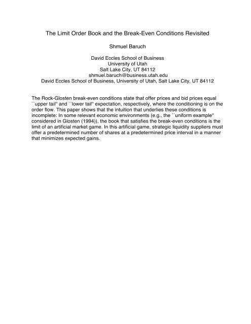
<strong>The</strong> <strong>Limit</strong> <strong>Order</strong> <strong>Book</strong> <strong>and</strong> <strong>the</strong> <strong>Break</strong>-<strong>Even</strong> Conditions Revisited<br />
Shmuel Baruch<br />
David Eccles <strong>School</strong> of Business<br />
University of Utah<br />
Salt Lake City, UT 84112<br />
shmuel.baruch@business.utah.edu<br />
David Eccles <strong>School</strong> of Business, University of Utah, Salt Lake City, UT 84112<br />
<strong>The</strong> Rock-Glosten break-even conditions state that offer prices <strong>and</strong> bid prices equal<br />
``upper tail'' <strong>and</strong> ``lower tail'' expectation, respectively, where <strong>the</strong> conditioning is on <strong>the</strong><br />
order flow. This paper shows that <strong>the</strong> intuition that underlies <strong>the</strong>se conditions is<br />
incomplete: In some relevant economic environments (e.g., <strong>the</strong> ``uniform example''<br />
considered in Glosten (1994)), <strong>the</strong> book that satisfies <strong>the</strong> break-even conditions is <strong>the</strong><br />
limit of an artificial market game. In this artificial game, strategic liquidity suppliers must<br />
offer a predetermined number of shares at a predetermined price interval in a manner<br />
that minimizes expected gains.
THE LIMIT ORDER BOOK AND THE BREAK-EVEN<br />
CONDITIONS REVISITED<br />
Abstract. <strong>The</strong> Rock-Glosten break-even conditions state that offer prices <strong>and</strong><br />
bid prices equal “upper tail” <strong>and</strong> “lower tail” expectation, respectively, where <strong>the</strong><br />
conditioning is on <strong>the</strong> order flow. This paper shows that <strong>the</strong> intuition that underlies<br />
<strong>the</strong>se conditions is incomplete: In some relevant economic environments (e.g.,<br />
<strong>the</strong> “uniform example” considered in Glosten (1994)), <strong>the</strong> book that satisfies <strong>the</strong><br />
break-even conditions is <strong>the</strong> limit of an artificial market game. In this artificial<br />
game, strategic liquidity suppliers must offer a predetermined number of shares at<br />
a predetermined price interval in a manner that minimizes expected gains.<br />
<strong>The</strong> assumption that liquidity suppliers break even provides a unifying framework for<br />
<strong>the</strong> literature on market microstructure. <strong>The</strong> break even conditions state that prices<br />
equal <strong>the</strong> expected value of <strong>the</strong> asset conditional on execution.<br />
In a market organized as a pure limit order book, a market order walks <strong>the</strong> book,<br />
picking off limit orders at <strong>the</strong>ir limit-prices. In that context, <strong>the</strong> liquidity suppliers are<br />
<strong>the</strong> limit order submitters. Following Rock (1990) <strong>and</strong> Glosten (1994), it is common<br />
to express <strong>the</strong> break even conditions in terms of upper <strong>and</strong> lower tail expectations of<br />
<strong>the</strong> asset value, where <strong>the</strong> conditioning is on <strong>the</strong> order flow.<br />
<strong>The</strong> goal of this paper is to reassess <strong>the</strong> Rock-Glosten break-even conditions.<br />
that end, we study a model of imperfect competition in liquidity provision <strong>and</strong> ask<br />
whe<strong>the</strong>r <strong>the</strong> competitive equilibrium is <strong>the</strong> limit of <strong>the</strong> model with a large number of<br />
liquidity suppliers.<br />
We consider economic environments where <strong>the</strong> profitability of a marginal offer depends<br />
only on its limit price <strong>and</strong> <strong>the</strong> cumulative depth up to that price. We model<br />
<strong>the</strong> interaction between <strong>the</strong> liquidity suppliers as a static game, as in Bernhardt <strong>and</strong><br />
Hughson (1997) <strong>and</strong> Biais, Martimort, <strong>and</strong> Rochet (2000). We <strong>the</strong>n use <strong>the</strong> principle<br />
of optimality to examine <strong>the</strong> problem of a liquidity supplier. 1 <strong>The</strong> Bellman equation<br />
can be used to construct a c<strong>and</strong>idate for equilibrium, <strong>and</strong> we see that <strong>the</strong> c<strong>and</strong>idate<br />
book satisfies, at <strong>the</strong> limit when <strong>the</strong> number of liquidity suppliers is large, <strong>the</strong><br />
Date: September, 2008.<br />
1 <strong>The</strong> problem is not dynamic in time. We just exploit <strong>the</strong> structure of <strong>the</strong> problem <strong>and</strong> use <strong>the</strong><br />
cumulative depth as <strong>the</strong> state variable.<br />
To<br />
1
2 THE LIMIT ORDER BOOK AND THE BREAK-EVEN CONDITIONS REVISITED<br />
Rock-Glosten conditions. However, it is not clear that <strong>the</strong> c<strong>and</strong>idate is indeed an<br />
equilibrium.<br />
<strong>The</strong> problem of a liquidity supplier is locally linear, which implies that <strong>the</strong> Bellman<br />
equation is degenerate. That is, we don’t know whe<strong>the</strong>r <strong>the</strong> c<strong>and</strong>idate for equilibrium<br />
is an outcome of a maximization or a minimization effort. We use Green’s <strong>the</strong>orem<br />
to state sufficient conditions for <strong>the</strong> c<strong>and</strong>idate to be an equilibrium. However, <strong>the</strong>se<br />
sufficient conditions are not merely technical, <strong>and</strong> in fact in some relevant economic<br />
environments <strong>the</strong> conditions are not satisfied.<br />
This leads us to consider an “artificial” market game, one where <strong>the</strong> goal of <strong>the</strong> liquidity<br />
suppliers is to minimize gains. In <strong>the</strong> artificial game, each liquidity suppliers must<br />
offer a prespecified number of shares in a prespecified price interval. <strong>The</strong> aggregate<br />
number of shares that must be offered equals <strong>the</strong> number of shares that are offered<br />
in <strong>the</strong> competitive equilibrium.<br />
In both market games, <strong>the</strong> realistic <strong>and</strong> <strong>the</strong> artificial, liquidity suppliers weigh in a<br />
similar manner <strong>the</strong> benefits <strong>and</strong> risks of placing aggressive offers. In <strong>the</strong> realistic<br />
market game, a liquidity supplier is reluctant to offer at aggressive prices because<br />
of <strong>the</strong> adverse selection risk. At <strong>the</strong> same time, <strong>the</strong> high precedence (thanks to <strong>the</strong><br />
price priority rule) increases <strong>the</strong> likelihood of trading against uninformed orders. <strong>The</strong><br />
optimal strategy balances this trade-off.<br />
In <strong>the</strong> artificial market game, <strong>the</strong> tradeoff is mirrored: a liquidity supplier is also<br />
reluctant to offer at aggressive prices, only that this time it is because of <strong>the</strong> potential<br />
gains from trading against uninformed orders. An aggressive offer, on <strong>the</strong> o<strong>the</strong>r h<strong>and</strong>,<br />
has <strong>the</strong> potential for large losses to informed orders. <strong>The</strong> optimal strategy in <strong>the</strong><br />
artificial game balances this trade-off.<br />
We consider several examples, in particular <strong>the</strong> two examples Glosten (1994) considers:<br />
<strong>the</strong> exponential-normal example <strong>and</strong> <strong>the</strong> uniform example. In <strong>the</strong> exponentialnormal<br />
example, we show that <strong>the</strong> Bellman equation characterizes <strong>the</strong> equilibrium of<br />
<strong>the</strong> realistic game. In contrast, in <strong>the</strong> uniform example, <strong>the</strong> Bellman equation characterizes<br />
<strong>the</strong> equilibrium of <strong>the</strong> artificial game. In particular, <strong>the</strong> competitive book<br />
that Glosten (1994) reports is <strong>the</strong> limit of <strong>the</strong> equilibrium book in <strong>the</strong> artificial game.<br />
It is possible that <strong>the</strong> Rock-Glosten conditions are satisfied at <strong>the</strong> limit of equilibria<br />
of <strong>the</strong> artificial trading game, computed via <strong>the</strong> Bellman equation, but that <strong>the</strong><br />
conditions are also satisfied at <strong>the</strong> limit of equilibria of <strong>the</strong> realistic game, even though
THE LIMIT ORDER BOOK AND THE BREAK-EVEN CONDITIONS REVISITED 3<br />
we may not know how to compute those equilibria. In that case, we should question<br />
<strong>the</strong> break-even conditions paradigm.<br />
An alternative explanation is that in some economic environments <strong>the</strong> break even<br />
conditions should not be expressed in terms of expectation conditional on <strong>the</strong> order<br />
flow, as Rock (1990) <strong>and</strong> Glosten (1994) posit. Baruch (2008) studies a variant of<br />
<strong>the</strong> uniform example <strong>and</strong> finds an equilibrium with r<strong>and</strong>om limit orders. When limit<br />
orders are r<strong>and</strong>om, <strong>the</strong>re is an additional uncertainty about <strong>the</strong> execution of a limit<br />
order. In o<strong>the</strong>r words, conditional on execution, a liquidity supplier cannot infer<br />
whe<strong>the</strong>r <strong>the</strong> incoming market order is large or <strong>the</strong> book is thin. Indeed, <strong>the</strong> limit of<br />
equilibria in Baruch (2008) does not satisfy <strong>the</strong> Rock-Glosten conditions.<br />
<strong>The</strong> paper is organized as follows. In Section 1 we describe <strong>the</strong> economic environment.<br />
In Section 2 we state <strong>the</strong> Rock-Glosten break even conditions. In Section 3 we define<br />
<strong>the</strong> equilibrium, <strong>and</strong> in Section 4 we use <strong>the</strong> Bellman equation to derive a c<strong>and</strong>idate for<br />
equilibrium. In Section 5 we provide sufficient conditions for equilibrium <strong>and</strong> present<br />
two examples. In Section 6 we define <strong>the</strong> artificial game <strong>and</strong> present examples. In<br />
Section 7 we conclude.<br />
1. <strong>The</strong> Economic Environment<br />
We model a pure limit order market for a single risky asset. <strong>The</strong>re are two types of<br />
traders in <strong>the</strong> model: risk neutral, uninformed liquidity suppliers <strong>and</strong> a single active<br />
trader. Initially, <strong>the</strong> liquidity suppliers populate <strong>the</strong> limit order book. Those limit<br />
orders are <strong>the</strong>n prioritized by <strong>the</strong>ir limit prices (i.e., price priority rule is enforced).<br />
Next, <strong>the</strong> active trader observes all <strong>the</strong> bids <strong>and</strong> offers in <strong>the</strong> book <strong>and</strong> submits a<br />
market order. Based on <strong>the</strong>ir priority, limit orders are matched with <strong>the</strong> market<br />
order until <strong>the</strong> market order is completly filled (i.e., <strong>the</strong> market order “walks <strong>the</strong><br />
book”), <strong>and</strong> trade takes place at <strong>the</strong> limit prices (i.e., trading against limit orders is<br />
discriminatory). Following <strong>the</strong> trade, <strong>the</strong> asset is liquidated; <strong>the</strong> liquidation value is<br />
ṽ. Without loss of generality, we focus on <strong>the</strong> offer side of <strong>the</strong> book. 2<br />
<strong>The</strong> ask price is <strong>the</strong> smallest price at which offers are posted. Let y(·) denote <strong>the</strong><br />
supply function; i.e., <strong>the</strong> liquidity suppliers offer y(x) shares up to <strong>the</strong> price x. By<br />
definition, y(·) is positive <strong>and</strong> increasing, <strong>and</strong> it is strictly positive above <strong>the</strong> ask price<br />
<strong>and</strong> strictly increasing at all those prices that are populated with offers. To emphasize<br />
that <strong>the</strong> active trader observes <strong>the</strong> supply function, we denote <strong>the</strong> order size by ˜δ(y(·)).<br />
2 We don’t lose generality because <strong>the</strong> liquidity suppliers are uninformed.
4 THE LIMIT ORDER BOOK AND THE BREAK-EVEN CONDITIONS REVISITED<br />
<strong>The</strong> tilde notation indicates that <strong>the</strong> order also depends on <strong>the</strong> trader’s unobservable<br />
characteristics (e.g. position in <strong>the</strong> asset) <strong>and</strong> possibly private information about <strong>the</strong><br />
liquidation value.<br />
Liquidity suppliers take into account <strong>the</strong> active trader’s behavior when posting <strong>the</strong>ir<br />
offers. In particular, given an arbitrary supply function, y(·), <strong>the</strong>y underst<strong>and</strong> <strong>the</strong><br />
joint distribution of <strong>the</strong> asset r<strong>and</strong>om value, ṽ, <strong>and</strong> <strong>the</strong> active trader’s order size,<br />
˜δ(y(·)).<br />
Consider a marginal offer at a price x when <strong>the</strong> supply function is y(·). <strong>The</strong> price<br />
priority rule implies that <strong>the</strong> offer is executed only if ˜δ(y(·)) > y(x). Because limit<br />
orders are filled at <strong>the</strong>ir limit prices, it follows that <strong>the</strong> ex post profitability of a<br />
marginal offer at a price x is given by: 3<br />
<strong>and</strong> <strong>the</strong> ex ante profitability is<br />
U(x, y(·)) = E(x−ṽ)I { e δ(y(·))>y(x)}<br />
=<br />
(x − ṽ)I { e δ(y(·))>y(x)}<br />
( [<br />
x − E ṽ<br />
∣<br />
∣˜δ(y(·)) > y(x)<br />
])<br />
Prob(˜δ(y(·)) > y(x))<br />
In this paper we restrict attention to economic environments in which <strong>the</strong> profitability<br />
of a marginal limit order depends only on its offer price <strong>and</strong> <strong>the</strong> cumulative number of<br />
shares offered up to that price. More specifically, <strong>the</strong>re are two continuous functions,<br />
defined on <strong>the</strong> <strong>the</strong> positive quadrant, ɛ(·, ·) <strong>and</strong> u(·, ·), such that for every pair (x, y(·)),<br />
we have EI { e δ(y(·))>y(x)}<br />
= ɛ(x, y(x)) <strong>and</strong> U(x, y(·)) = u(x, y(x)). We refer to u(x, y) as<br />
<strong>the</strong> profitability of a marginal offer at (x, y); i.e. <strong>the</strong> profitability of a marginal offer at<br />
x when y shares are offered at prices better than x. Similarly, ɛ(x, y) is <strong>the</strong> probability<br />
of execution of a marginal offer at (x, y).<br />
Let D = {(x, y) : ɛ(x, y) > 0} be <strong>the</strong><br />
“relevant region:” marginal offers at (x, y) /∈ D are never filled up. We assume that<br />
u(·, ·) is smooth in <strong>the</strong> relevant region. Intuitively, <strong>the</strong> smoothness requirement means<br />
that <strong>the</strong> distribution functions of all r<strong>and</strong>om variables that underly <strong>the</strong> economic<br />
environment (e.g. asset value) are smooth.<br />
We conclude this section with some examples. Each example illustrates an economic<br />
environment where we can calculate explicitly <strong>the</strong> function u(·, ·) <strong>and</strong> <strong>the</strong> “relevant”<br />
region D.<br />
<strong>The</strong> Exponential Example:<br />
3 Because y(x) is <strong>the</strong> number of shares offered up to x, it follows that if y(·) has jump at x, <strong>the</strong>n<br />
<strong>the</strong> expression reflects <strong>the</strong> profitability of <strong>the</strong> “first unit” offered at x. This paper studies equilibria<br />
with continuous supply functions.
THE LIMIT ORDER BOOK AND THE BREAK-EVEN CONDITIONS REVISITED 5<br />
<strong>The</strong> liquidation value of <strong>the</strong> asset is ṽ = ˜s + ˜ɛ. An active trader with an exponential<br />
utility observes <strong>the</strong> signal ˜s. <strong>The</strong> trader’s initial position in <strong>the</strong> asset is Ĩ. <strong>The</strong> noise<br />
term, ˜ɛ, is a zero mean normal r<strong>and</strong>om variable with variance σ 2 , <strong>and</strong> ˜ɛ is independent<br />
of ˜s <strong>and</strong> Ĩ.<br />
Given all <strong>the</strong> bids <strong>and</strong> offers in <strong>the</strong> book, let t(δ) denote <strong>the</strong> marginal price of an<br />
order of size δ. That is, if δ < 0, <strong>the</strong>n t(δ) is <strong>the</strong> proceeds for selling <strong>the</strong> last fraction<br />
of <strong>the</strong> order, <strong>and</strong> if δ > 0 <strong>the</strong>n t(δ) is <strong>the</strong> cost of <strong>the</strong> last fraction. Because of <strong>the</strong> price<br />
priority rule, <strong>the</strong> function t(·) is non-decreasing, <strong>and</strong> <strong>the</strong>refore ∫ δ<br />
t(z)dz is convex.<br />
0<br />
<strong>The</strong> trader infers t(·) from y(·) <strong>and</strong> submits a market order of size δ that maximizes 4<br />
[<br />
]<br />
E − exp(−γ˜W ) ∣ I, s<br />
where ˜W = (δ + I)(s + ˜ɛ) − ∫ δ<br />
t(z)dz. Because of <strong>the</strong> exponential utility function,<br />
0<br />
<strong>the</strong> investor’s problem is equivalent to <strong>the</strong> concave problem:<br />
where θ = s − γσ 2 I. 5<br />
max θδ − γ σ2<br />
δ 2 δ2 −<br />
∫ δ<br />
0<br />
t(z)dz<br />
If <strong>the</strong> optimal size turns out to be strictly positive, <strong>the</strong>n it<br />
equals sup{δ : θ − γσ 2 δ − t(δ) > 0}, or equivalently, <strong>the</strong> order walks up <strong>the</strong> book as<br />
long as θ > γσ 2 y(x) + x. 6<br />
<strong>The</strong> liquidity suppliers don’t observe θ, but <strong>the</strong>y underst<strong>and</strong> <strong>the</strong> active trader’s strategy.<br />
Let F (·) be <strong>the</strong> distribution function of ˜θ, v(θ) = E[ṽ|˜θ = θ], <strong>and</strong> v + (θ) =<br />
E[ṽ|˜θ > θ]. <strong>The</strong> profitability of a marginal offer is <strong>the</strong>n<br />
u(x, y) = E(x − ṽ)I { e θ>γσ 2 y+x}<br />
= x ( 1 − F ( γσ 2 y + x )) −<br />
∫ ∞<br />
x+y<br />
v(θ)dF (θ)<br />
= ( x − v + ( γσ 2 y + x )) ( 1 − F ( γσ 2 y + x )) .<br />
In Biais, Martimort, <strong>and</strong> Rochet (2000), <strong>the</strong> support of ˜s <strong>and</strong> Ĩ are are closed intervals.<br />
<strong>The</strong> relevant region is D = {(x, y) : x + γσ 2 y < ¯θ}, where ¯θ is <strong>the</strong> upper support of<br />
˜θ. <strong>The</strong> probability of execution is ɛ(x, y) = 1 − F (γσ 2 y + x).<br />
4 Wherever y(·) is invertible (i.e., prices at which <strong>the</strong> supply function is strictly monotone), its inverse<br />
is t(·).<br />
5 In Glosten’s (1994) terminology, <strong>the</strong> informed trader’s marginal valuation is θ − γσ 2 δ.<br />
6 <strong>The</strong> objective function of <strong>the</strong> concave problem may not be smooth because t(·) may not be continuous<br />
(for example, if <strong>the</strong> spread is strictly positive <strong>the</strong>n at zero t(·) has a point of discontinuity).<br />
<strong>The</strong> argument we invoke is that <strong>the</strong> optimal size is greater than any size at which <strong>the</strong> derivative of<br />
<strong>the</strong> objective function is strictly positive. And this is true because <strong>the</strong> problem is concave.
6 THE LIMIT ORDER BOOK AND THE BREAK-EVEN CONDITIONS REVISITED<br />
In Glosten (1994), ˜s <strong>and</strong> Ĩ are assumed to be independent <strong>and</strong> normally distributed,<br />
<strong>and</strong> in particular D is <strong>the</strong> positive quadrant.<br />
<strong>The</strong> Uniform Example:<br />
We now consider an economic environment in which with probability µ <strong>the</strong> active<br />
trader is an uninformed trader who wants to buy at most ˜k shares up to <strong>the</strong> reservation<br />
price ˜p. With probability 1 − µ <strong>the</strong> active trader is an informed trader. In that case,<br />
<strong>the</strong> trader observes <strong>the</strong> true value of <strong>the</strong> asset, ṽ, <strong>and</strong> picks off all offers below ṽ <strong>and</strong><br />
all bids above ṽ.<br />
<strong>The</strong> ex ante profitability of a marginal offer is <strong>the</strong>refore<br />
]<br />
u(x, y) = E<br />
[(1 − µ)(x − ṽ)I {ev>x} + µ(x − Eṽ)I {ep>x, e k>y}<br />
= (1 − µ)E(x − ṽ)I {ev>x} + µ(x − Eṽ)EI {ep>x, e k>y}<br />
In <strong>the</strong> uniform example in Glosten (1994), <strong>the</strong> liquidation value is uniformly distributed<br />
over [−L, L], <strong>and</strong> <strong>the</strong> joint distribution of ˜p <strong>and</strong> ˜k satisfies 7<br />
⎧<br />
⎨ L−(x+y)<br />
x + y ≤ L<br />
2L<br />
EI {ep>x, e k>y}<br />
=<br />
⎩0 x + y > L<br />
Hence, in <strong>the</strong> uniform example, <strong>the</strong> ex ante expected profit of a marginal offer is given<br />
by<br />
⎧<br />
⎨− 1−µ<br />
(1) u(x, y) =<br />
(L − 4L x)2 + µ x(L − (x + y)) x + y ≤ L<br />
2L<br />
⎩0 x + y > L<br />
<strong>The</strong> relevant region is D = {(x, y) : x + y < L}, <strong>and</strong> <strong>the</strong> probability of execution is<br />
ɛ(x, y) = (1 − µ) L − x<br />
2L<br />
+ µL<br />
− (x + y)<br />
2L<br />
<strong>The</strong> Inelastic Dem<strong>and</strong> Example:<br />
In this economic environment, <strong>the</strong> size of <strong>the</strong> active trader’s order is a sufficient<br />
statistic about <strong>the</strong> asset value. Let F (δ) be <strong>the</strong> cumulative distribution function of<br />
7 In o<strong>the</strong>r words, an uninformed trader’s order walks up <strong>the</strong> book as long as ˜ɛ > x + y(x) where ˜ɛ<br />
is uniformly distributed [−L, L]. In Glosten’s terminology, <strong>the</strong> marginal valuation of an uninformed<br />
trader is ɛ − y(x).
THE LIMIT ORDER BOOK AND THE BREAK-EVEN CONDITIONS REVISITED 7<br />
<strong>the</strong> order size, v(δ) = E[ṽ|˜δ = δ], <strong>and</strong> v + (δ) = E[ṽ|˜δ > δ]. <strong>The</strong> expected profit of a<br />
marginal offer is<br />
u(x, y) = E(x − ṽ)I { δ>y} e = x(1 − F (y)) −<br />
= (x − v + (y))(1 − F (y))<br />
∫ ∞<br />
y<br />
v(u)dF (u)<br />
<strong>The</strong> relevant region is D = {(x, y) : F (y) < 1}, <strong>and</strong> <strong>the</strong> probability of execution is<br />
ɛ(x, y) = (1 − F (y)).<br />
2. <strong>The</strong> <strong>Break</strong> <strong>Even</strong> Conditions<br />
Following Rock (1990) <strong>and</strong> Glosten (1994), it is common to posit that when <strong>the</strong>re<br />
are infinitely many liquidity suppliers <strong>and</strong> it is costless to post offers <strong>the</strong>n <strong>the</strong> supply<br />
function satisfies <strong>the</strong> break even conditions:<br />
[<br />
]<br />
x ≤ E ṽ|˜δ(y(·)) > y(x)<br />
with equality whenever dy(x) > 0. <strong>The</strong> right h<strong>and</strong> side is commonly called <strong>the</strong> “upper<br />
tail expectation.” We may have a strict inequality because <strong>the</strong>re are prices at which<br />
even competitive liquidity suppliers do not offer shares (e.g., prices that are below<br />
<strong>the</strong> ask price).<br />
An economic environment is said to be regular if: (i) <strong>The</strong>re is a unique supply function,<br />
which we denote by y ∞ (·), that satisfies <strong>the</strong> break even condition, <strong>and</strong> (ii) In <strong>the</strong><br />
relevant region D, <strong>the</strong> sign of u(·, ·) is negative above <strong>the</strong> graph of y ∞ (x) <strong>and</strong> positive<br />
below <strong>the</strong> graph. 8 We denote by ask ∞ <strong>the</strong> ask price that corresponds to <strong>the</strong> supply<br />
function y ∞ (·).<br />
Though our analysis is general, we are only interested in regular economic environments<br />
where <strong>the</strong> argument for <strong>the</strong> break even conditions sounds appealing. In a<br />
regular economic environment, <strong>the</strong> following procedure can be used to construct <strong>the</strong><br />
supply function y ∞ (·): ask ∞ is <strong>the</strong> smallest positive root of x → u(x, 0). For all<br />
x < ask ∞ , we set y ∞ (x) = 0. For all x > ask ∞ , we set y ∞ (x) to be <strong>the</strong> value where<br />
<strong>the</strong> function y → u(x, y) changes signs.<br />
8 <strong>The</strong> graph of y ∞ (·) is a subset of <strong>the</strong> positive quadrant: it is <strong>the</strong> collection of all <strong>the</strong> pairs (x, y ∞ (x)).
8 THE LIMIT ORDER BOOK AND THE BREAK-EVEN CONDITIONS REVISITED<br />
3. Equilibrium with n Strategic Liquidity suppliers<br />
We follow <strong>the</strong> modeling choice of Bernhardt <strong>and</strong> Hughson (1997) <strong>and</strong> Biais, Martimort,<br />
<strong>and</strong> Rochet (2000), <strong>and</strong> model <strong>the</strong> interaction between <strong>the</strong> liquidity suppliers<br />
as a game with n strategic liquidity suppliers who post offers simultaneously.<br />
For technical reasons, we make <strong>the</strong> assumption that <strong>the</strong>re is an exogenous maximum<br />
price X at which offers can be posted. With X we associate<br />
∫ y<br />
(2) Y = argmax u(X, u)du<br />
y<br />
In a regular economic environment, if X < ask ∞ , <strong>the</strong>n no offers will be posted. If<br />
X > ask ∞ <strong>and</strong> (X, Y ) is in <strong>the</strong> relevant region D, <strong>the</strong>n <strong>the</strong> profit of a marginal offer<br />
at (X, Y ) is zero; i.e., without incurring a loss, liquidity providers cannot offer more<br />
than Y shares at X. 9<br />
We let q i (·) denote <strong>the</strong> marginal supply function of <strong>the</strong> i-th liquidity supplier, <strong>and</strong> set<br />
q −i (·) = ∑ j≠i q j(·): In <strong>the</strong> price interval (x, x + dx), <strong>the</strong> i-th liquidity supplier offers<br />
q i (x)dx shares. If y(x) shares are offered by all liquidity suppliers at prices up to x,<br />
<strong>the</strong>n <strong>the</strong> ex ante profit is u(x, y(x))q i (x)dx <strong>and</strong> at x + dx, <strong>the</strong> total number of shares<br />
offered is y(x + dx) = y(x) + (q i (x) + q −i (x))dx. This means that <strong>the</strong> problem of <strong>the</strong><br />
i-th liquidity supplier can be written as<br />
(3)<br />
⎧ ∫ X<br />
max u(x, y(x))q(x)dx<br />
q(x)≥0<br />
0<br />
⎪⎨<br />
subject to<br />
dy(x) = (q −i (x) + q(x))dx<br />
⎪⎩<br />
y(0) = 0<br />
Implicit in <strong>the</strong> <strong>the</strong> setting of <strong>the</strong> problem is <strong>the</strong> assumption that no discrete offers are<br />
posted. However, we don’t impose any upper bound on q(x). Thus, if it is optimal to<br />
offer a discrete offer, <strong>the</strong>n we will not be able to find a solution to this maximization<br />
problem.<br />
An equilibrium is an n-tuple of functions (q 1 (·), q 2 (·), . . . , q n (·)) such that for every<br />
i, q i (·) solves problem (3). A symmetric equilibrium is an equilibrium in which all<br />
liquidity suppliers use <strong>the</strong> same marginal supply function.<br />
9 We guess that in a model with endogenous maximum price, X would be <strong>the</strong> highest price at which<br />
<strong>the</strong> supply function y ∞ (·) is strictly increasing.
THE LIMIT ORDER BOOK AND THE BREAK-EVEN CONDITIONS REVISITED 9<br />
4. <strong>The</strong> Bellman Equation<br />
In this section, we use <strong>the</strong> Bellman equation to informally derive a necessary condition<br />
for an equilibrium in which for all i, q i (·) is finite <strong>and</strong> strictly positive above <strong>the</strong> ask<br />
price. <strong>Even</strong> though <strong>the</strong> problem of a liquidity supplier is static, we can never<strong>the</strong>less<br />
use <strong>the</strong> principle of optimality, as if a liquidity supplier first chooses how many shares<br />
to offer at aggressive prices.<br />
Define<br />
⎧ ∫ X<br />
max<br />
q(x)≥0<br />
x 0<br />
u(x, y)q(x)dx<br />
⎪⎨<br />
subject to<br />
v(x 0 , y 0 ) =<br />
dy = q −i (x) + q(x)dx<br />
⎪⎩<br />
y(x 0 ) = y 0<br />
<strong>The</strong> Bellman equation is<br />
max<br />
q≥0 v x + v y (q −i (x) + q) + u(x, y)q = 0.<br />
Because <strong>the</strong> problem is linear in q, we must have<br />
v y = − u(x, y)<br />
v x = − v y q −i (x) = q −i (x)u(x, y)<br />
Now, differentiate <strong>the</strong> first equation by x <strong>and</strong> <strong>the</strong> second by y, to get<br />
v yx = − u x (x, y)<br />
v xy =q −i (x)u y (x, y)<br />
So, for <strong>the</strong> trader to have an optimal positive solution, <strong>the</strong> equilibrium supply function<br />
must solve <strong>the</strong> equation<br />
q −i (x) = − u x(x, y(x))<br />
u y (x, y(x))<br />
This must hold for every trader, <strong>and</strong> moreover <strong>the</strong> right h<strong>and</strong> side is independent of<br />
i.<br />
We conclude that <strong>the</strong> equilibrium is symmetric, <strong>and</strong> <strong>the</strong> supply function solves <strong>the</strong><br />
o.d.e.<br />
(4)<br />
dy<br />
dx = − n u x (x, y)<br />
n − 1 u y (x, y) ,<br />
y(X) = Y
10 THE LIMIT ORDER BOOK AND THE BREAK-EVEN CONDITIONS REVISITED<br />
in <strong>the</strong> interval [ask, X]. In a regular economic environment, <strong>the</strong> boundary condition<br />
is natural: to offer less than Y shares would mean to leave money on <strong>the</strong> table, while<br />
to offer more than Y would imply losses.<br />
Note that if we denote by y n (·) <strong>the</strong> solution to (4), <strong>the</strong>n intuitively we see that y n (·)<br />
is an increasing sequence of functions (i.e., y n (x) ≤ y n+1 (x)), <strong>and</strong> lim n→∞ y n (·) is <strong>the</strong><br />
solution to <strong>the</strong> o.d.e. 10<br />
dy<br />
dx = −u x(x, y)<br />
u y (x, y) , y(X) = Y<br />
which is given implicitly by equation u(x, y(x)) = 0; i.e., <strong>the</strong> break even conditions<br />
are satisfied at <strong>the</strong> limit.<br />
Before leaving this section, we make <strong>the</strong> following observation.<br />
Nowhere, in <strong>the</strong><br />
analysis above, have we used <strong>the</strong> fact that <strong>the</strong> objective is to maximize gains, ra<strong>the</strong>r<br />
than say minimize <strong>the</strong>m. Moreover, because <strong>the</strong> Bellman equation is linear in q,<br />
<strong>the</strong>re are no second order conditions that can be checked. <strong>The</strong> st<strong>and</strong>ard approach<br />
in dynamic programming is to use <strong>the</strong> value function to verify <strong>the</strong> solution. Here,<br />
however, <strong>the</strong> value function is only identified along <strong>the</strong> “equilibrium path.” That is,<br />
we know v(x, y(x)), ra<strong>the</strong>r than v(x, y) for arbitrary pairs of (x, y). We <strong>the</strong>refore have<br />
to use a different approch to verify <strong>the</strong> equilibrium. We do so in <strong>the</strong> next section.<br />
5. A verification <strong>The</strong>orem<br />
Given a strictly monotone solution to <strong>the</strong> o.d.e.<br />
(4), we want to verify that <strong>the</strong><br />
solution indeed defines <strong>the</strong> equilibrium. Let ask n be <strong>the</strong> first price, when we solve<br />
<strong>the</strong> o.d.e. (4) backward, at which <strong>the</strong> solution intercepts <strong>the</strong> x axis. Let y ∗ (·) denote<br />
<strong>the</strong> solution to <strong>the</strong> backward differential equation (4) in <strong>the</strong> interval [ask n , X]. For<br />
x < ask n , set y ∗ (x) = 0. Let<br />
⎧<br />
⎨0, x < ask<br />
q ∗ n<br />
(x) =<br />
⎩ u x(x,y ∗ (x))<br />
ask n ≤ x ≤ X<br />
− 1 ,<br />
n−1 u y(x,y ∗ (x))<br />
so that y ∗ (x) = ∫ x<br />
0 nq∗ (u)du. Finally, define Miele’s fundamental function<br />
ω ∗ (x, y) = u x (x, y) + u y (x, y)(n − 1)q ∗ (x)<br />
<strong>The</strong>orem 1. If (i) u(·, ·) is smooth in <strong>the</strong> relevant region D, (ii) y ∗ (·) as defined above<br />
is strictly increasing above <strong>the</strong> ask price (in particular, <strong>the</strong>re is a solution to <strong>the</strong> o.d.e.<br />
(4)), <strong>and</strong> (iii) in <strong>the</strong> relevant region, <strong>the</strong> sign of Miele’s function is negative below<br />
10 To make this statement rigorous, one has to impose additional technical assumptions on <strong>the</strong><br />
function u(·, ·).
THE LIMIT ORDER BOOK AND THE BREAK-EVEN CONDITIONS REVISITED 11<br />
<strong>the</strong> graph of y ∗ (·) <strong>and</strong> positive above <strong>the</strong> graph of y ∗ (·), <strong>the</strong>n q ∗ (·) forms a symmetric<br />
equilibrium <strong>and</strong> y ∗ (·) is <strong>the</strong> equilibrium supply function.<br />
To intuitively underst<strong>and</strong> <strong>the</strong> role of Miele’s function, we recall a st<strong>and</strong>ard result<br />
from calculus that is usuful when <strong>the</strong> first order conditions fail. Consider an arbitrary<br />
continuous function that is piecewise differentiable, f(·). If we were to plot <strong>the</strong> sign<br />
of f ′ (·) in an interval [a, b], <strong>and</strong> find an x ∈ [a, b] such that in [a, x), <strong>the</strong> sign of f ′ (·) is<br />
positive <strong>and</strong> in (x, b] <strong>the</strong> sign is negative, <strong>the</strong>n x maximizes f(·) in <strong>the</strong> interval. <strong>Even</strong><br />
if x is at <strong>the</strong> corner of <strong>the</strong> interval or f ′ (x) does not exist (i.e., <strong>the</strong> local conditions<br />
for optimality fail), x is <strong>the</strong> optimal. This result is a consequence of <strong>the</strong> fundamental<br />
<strong>the</strong>orem of calculus: for any z ∈ [a, b], f(x) − f(z) = ∫ x<br />
z f ′ (u)du > 0.<br />
In <strong>the</strong> proof of <strong>The</strong>orem 1, we express <strong>the</strong> objective of a liquidity supplier as a line<br />
integral, where <strong>the</strong> goal is to choose <strong>the</strong> curve that maximizes <strong>the</strong> line integral along<br />
<strong>the</strong> curve. <strong>The</strong> difference between <strong>the</strong> payoff of two curves can be expressed as <strong>the</strong><br />
line integral along a closed curve. Miele’s function is analogous to <strong>the</strong> derivative of <strong>the</strong><br />
line integral, <strong>and</strong> <strong>the</strong>refore we are interested in <strong>the</strong> sign of Miele’s function. To verify<br />
optimality, we use Green’s <strong>the</strong>orem, which is essentially a two dimensional version of<br />
<strong>the</strong> fundamental <strong>the</strong>orem of calculus: Green’s <strong>the</strong>orem equates <strong>the</strong> line integral along<br />
a closed curve with <strong>the</strong> double integral of Miele’s function in <strong>the</strong> region enclosed by<br />
<strong>the</strong> curve; i.e., <strong>the</strong> difference in payoffs between two curves that start at common<br />
point <strong>and</strong> end at a common point. 11<br />
Before we prove <strong>the</strong> <strong>the</strong>orem, we show how we apply <strong>the</strong> <strong>the</strong>orem in two examples.<br />
<strong>The</strong> Exponential-Normal Example:<br />
Glosten (1994) studies a special case of <strong>the</strong> exponential example, in which<br />
Ĩ <strong>and</strong> ˜s<br />
are normally distributed with zero mean, <strong>the</strong> variance of Ĩ is α < 1, <strong>the</strong> variance of<br />
˜s is 1 − α, <strong>and</strong> σ = γ = 1, so that ˜θ is a st<strong>and</strong>ard normal r<strong>and</strong>om variable. We have<br />
v(θ) = (1 − α)θ<br />
<strong>and</strong><br />
v + ϕ(θ)<br />
(θ) = (1 − α)<br />
1 − Φ(θ)<br />
where ϕ(·) <strong>and</strong> Φ(·) are <strong>the</strong> density function <strong>and</strong> <strong>the</strong> cumulative distribution function<br />
of a st<strong>and</strong>ard normal r<strong>and</strong>om variable, respectively. Thus, u(x, y) is given by<br />
u(x, y) = x(1 − Φ(y + x)) − (1 − α)ϕ(y + x).<br />
11 In <strong>the</strong> Appendix we prove a simple version of Green’s <strong>the</strong>orem. <strong>The</strong> proof is an application of <strong>the</strong><br />
fundamental <strong>the</strong>orem of calculus.
12 THE LIMIT ORDER BOOK AND THE BREAK-EVEN CONDITIONS REVISITED<br />
We set <strong>the</strong> parameters: α = 0.8 <strong>and</strong> X = 0.9. Because y → u(X, y) changes signs<br />
only once, Y is <strong>the</strong> <strong>the</strong> root of <strong>the</strong> equation u(0.9, y) = 0. We solve <strong>and</strong> find that<br />
Y = 3.387092. Next we solve <strong>the</strong> o.d.e. (4) by integrating backward until <strong>the</strong> solution<br />
vanishes. Figure (1) shows <strong>the</strong> solution for different number of value traders. In<br />
particular, <strong>the</strong> supply function is monotone, as required in <strong>the</strong> <strong>the</strong>orem. Thus, to<br />
verify that we have found <strong>the</strong> equilibrium, we only need to check that <strong>the</strong> sign of<br />
ω ∗ (·, ·) is positive above <strong>the</strong> graph of y ∗ (·) <strong>and</strong> negative below it. Figure (2) shows<br />
that this is indeed <strong>the</strong> case.<br />
y(x)<br />
3<br />
2.5<br />
2<br />
1.5<br />
1<br />
0.5<br />
“n = ∞”<br />
n = 5<br />
n = 2<br />
0.3 0.6 0.9<br />
x<br />
Figure 1. Equilibrium Supply Function in <strong>the</strong> Exponential-Normal Example.<br />
<strong>The</strong> figure shows <strong>the</strong> equilibrium supply function in <strong>the</strong> exponential<br />
normal case for different number of value traders. <strong>The</strong> parameters are<br />
α = 0.8 <strong>and</strong> X = 0.9, <strong>and</strong> n is ei<strong>the</strong>r 2, 5 or <strong>the</strong> limiting case that satisfies<br />
<strong>the</strong> break even conditions (“n = ∞”).<br />
<strong>The</strong> Inelastic Dem<strong>and</strong> Example:<br />
Assume <strong>the</strong> active trader’s orders size is uniformly distributed over <strong>the</strong> unit interval,<br />
<strong>and</strong> v(δ) = δ. <strong>The</strong> relevant region is <strong>the</strong> open rectangle {(x, y) : 0 ≤ x, 0 ≤ y ≤ 1}<br />
<strong>and</strong><br />
⎧<br />
⎨x(1 − y) − 1/2 + y 2 /2 y ≤ 1<br />
u(x, y) =<br />
⎩0 y > 1
THE LIMIT ORDER BOOK AND THE BREAK-EVEN CONDITIONS REVISITED 13<br />
ω(x, y)<br />
ω(x, y)<br />
0.4<br />
0.4<br />
0<br />
0<br />
−0.4<br />
−0.8<br />
0 0.45 0.9<br />
x<br />
0<br />
1.69<br />
y<br />
3.38<br />
−0.4<br />
−0.8<br />
0 0.45 0.9<br />
x<br />
0<br />
1.69<br />
y<br />
3.38<br />
Figure 2. Miele’s Function in <strong>the</strong> Exponential-Normal Example. <strong>The</strong><br />
equilibrium supply function, y ∗ (·) is depicted n <strong>the</strong> plane (x, y, 0). For better<br />
visualization, in <strong>the</strong> right panel we also show <strong>the</strong> surface (x, y, 0). It can be<br />
seen that for every pair (x, y) above (below) <strong>the</strong> graph of y ∗ (·), sgn ω ∗ (x, y)<br />
is positive (negative). <strong>The</strong> parameters are α = 0.8 <strong>and</strong> X = 0.9 <strong>and</strong> n = 5.<br />
Set <strong>the</strong> maximum price X = 1, <strong>and</strong> solve u(1, y) = 0 to find that Y = 1. <strong>The</strong> solution<br />
of <strong>the</strong> backward differential equation (4) is linear:<br />
y(x) = x 2n − 1<br />
n − 1 − n<br />
n − 1<br />
<strong>The</strong> ask price is<br />
ask n =<br />
n<br />
2n − 1<br />
hence <strong>the</strong> supply function is<br />
⎧<br />
⎨0, 0 ≤ x < n<br />
y ∗ 2n−1<br />
(x) =<br />
⎩x 2n−1 − n , n<br />
≤ x ≤ 1<br />
n−1 n−1 2n−1<br />
To verify that this is <strong>the</strong> equilibrium supply function, note that in <strong>the</strong> relevant region<br />
(i.e. y ≤ 1) Miele’s function is<br />
⎧<br />
⎨1 − y, 0 ≤ x < ask<br />
ω ∗ n<br />
(x, y) =<br />
⎩(1 − y) − (y − x) (1−2n) , ask<br />
n n ≤ x ≤ 1<br />
⎧<br />
⎨1 − y, 0 ≤ x < ask n<br />
=<br />
⎩ n<br />
(y − n−1 y∗ (x)) , ask n ≤ x ≤ 1<br />
Because for every price x below <strong>the</strong> ask price, y(x) = 0, we see that in D, ω ∗ (x, y) is<br />
positive above <strong>the</strong> graph of y ∗ (x) <strong>and</strong> negative below it. Thus, we have verified <strong>the</strong><br />
equilibrium in this example.
14 THE LIMIT ORDER BOOK AND THE BREAK-EVEN CONDITIONS REVISITED<br />
Proof of <strong>The</strong>orem 1: Assume <strong>the</strong> conditions in <strong>the</strong> <strong>the</strong>orem hold, <strong>and</strong> n − 1 value<br />
traders use <strong>the</strong> strategy q ∗ (·). We need to show that q ∗ (·) is optimal for <strong>the</strong> n-th<br />
trader as well. Because y ∗ (·) is monotone, q ∗ (·) is a feasible strategy.<br />
By inserting, in (3), <strong>the</strong> constraint into <strong>the</strong> objective, we remove q(·) from <strong>the</strong> objective<br />
<strong>and</strong> express <strong>the</strong> payoff in terms of y(·):<br />
∫ X<br />
0<br />
u(x, y(x))dy(x) −<br />
∫ X<br />
0<br />
u(x, y(x))(n − 1)q ∗ (x)dx<br />
We note that <strong>the</strong> above is also <strong>the</strong> line integral of u(x, y)dy − u(x, y)(n − 1)q ∗ (x)dx<br />
along <strong>the</strong> graph of y(·). Thus, <strong>the</strong> payoff of every strategy q(·) equals <strong>the</strong> line integral<br />
along <strong>the</strong> graph of y(·), where y(x) = ∫ x<br />
0 q∗ −i(s) + q(s)ds.<br />
Let C denote a plane curve <strong>and</strong> let<br />
∫<br />
(5) I(C) = u(x, y)dy − u(x, y)(n − 1)q ∗ (x)dx<br />
C<br />
We denote <strong>the</strong> graph of <strong>the</strong> function y ∗ (·) by C y ∗. To prove that q ∗ (·) forms a<br />
symmetric equilibrium, it is sufficient to show that I(C y ∗) ≥ I(C) for every plane<br />
curve that lies in relevant region D, starts at <strong>the</strong> origin, <strong>and</strong> ends at a point on <strong>the</strong><br />
vertical line x = X. <strong>The</strong> proof that it is sufficient to restrict attention to D is given<br />
in Lemma 1 in <strong>the</strong> Appendix. 12<br />
Consider a plane curve that lies above <strong>the</strong> graph of y ∗ (·), as shown in Figure (3). Let<br />
α consist of all those points that are above <strong>the</strong> graph of y ∗ (·) <strong>and</strong> below C. Let ∂α<br />
be <strong>the</strong> positively-oriented simple closed curve that forms <strong>the</strong> boundary of α; 13 i.e.,<br />
∂α is <strong>the</strong> union of C y ∗, <strong>the</strong> vertical plane curve that connects C y ∗ to C, <strong>and</strong> −C. 14<br />
∮<br />
∫∫<br />
I(C y ∗) − I(C) ≥ u(x, y)dy − u(x, y)(n − 1)q ∗ (x)dx = ω ∗ (x, y)dxdy ≥ 0<br />
∂α<br />
α<br />
12 This problem is more general than <strong>the</strong> original problem: 1) We don’t require that <strong>the</strong> graph be<br />
above <strong>the</strong> graph of <strong>the</strong> function y ∗ (·)(n − 1)/n. We ignore this condition because it was never<br />
binding is specific examples. 2) We don’t require <strong>the</strong> arbitrary plane curve be <strong>the</strong> graph of a<br />
monotone function or a smooth function or even a continuous function.<br />
13 A simple closed curve is said to be positively oriented if, as we traverse <strong>the</strong> curve, <strong>the</strong> region<br />
enclosed by <strong>the</strong> curve is to our left. <strong>The</strong> arrows in Figure (3) indicate <strong>the</strong> directions.<br />
14 <strong>The</strong> minus sign before C indicates <strong>the</strong> reversal of orientation on C.
THE LIMIT ORDER BOOK AND THE BREAK-EVEN CONDITIONS REVISITED 15<br />
y<br />
C<br />
<<br />
<<br />
(X, Y )<br />
<<br />
α<br />
><br />
ω ∗ > 0<br />
C y ∗<br />
ω ∗ < 0<br />
><br />
><br />
X<br />
x<br />
Figure 3. Green’s <strong>The</strong>orem <strong>and</strong> <strong>the</strong> optimality of C y ∗. <strong>The</strong> sign of ω ∗ (·, ·)<br />
is negative in <strong>the</strong> shaded area <strong>and</strong> positive elswhere. <strong>The</strong> difference in <strong>the</strong><br />
value of <strong>the</strong> line integral (5) along C y ∗ <strong>and</strong> <strong>the</strong> line integral along C is greater<br />
than <strong>the</strong> double integral of ω ∗ (·, ·) in <strong>the</strong> region α. Because ω ∗ (·, ·) is positive<br />
in α, <strong>the</strong> double integral is positive.<br />
where <strong>the</strong> first inequality is from <strong>the</strong> definition of Y . 15 <strong>The</strong> second equality is Green’s<br />
<strong>The</strong>orem, 16 <strong>and</strong> <strong>the</strong> final inequality is because <strong>the</strong> sign of ω ∗ (·, ·) is positive in α.<br />
We now consider a plane curve C as depicted in Figure (4). Let α be <strong>the</strong> set of points<br />
that are above C y ∗ <strong>and</strong> below C, <strong>and</strong> let β be <strong>the</strong> set of points that are below C y ∗ <strong>and</strong><br />
above C. Let ∂α <strong>and</strong> ∂β be <strong>the</strong> positively-oriented simple closed curves that forms<br />
15 <strong>The</strong> definition of Y implies that <strong>the</strong> line integral (5) is negative for any vertical curve that starts<br />
at (X, Y ). Indeed, <strong>the</strong> a vertical plane curve, C, starts at (X, Y ) <strong>and</strong> ends in (X, Y ′ ). Because<br />
Y ∫<br />
′<br />
“dx = 0,” we have I(C) = u(X, y)dy ≤ 0.<br />
Y<br />
16 In Appendix B, we prove that Green’s <strong>The</strong>orem can be applied even though <strong>the</strong> integr<strong>and</strong> is not<br />
smooth: q ∗ (·) has a point of discontinuity at x = ask, <strong>and</strong> ω ∗ (·, ·) has a vertical curve of discontinuity<br />
at x = ask.
16 THE LIMIT ORDER BOOK AND THE BREAK-EVEN CONDITIONS REVISITED<br />
y<br />
(X, Y )<br />
ω ∗ > 0<br />
<<br />
><br />
β<br />
<<br />
<<br />
α<br />
C<br />
><br />
C y ∗<br />
ω ∗ < 0<br />
X<br />
x<br />
Figure 4. Green’s <strong>The</strong>orem <strong>and</strong> <strong>the</strong> optimality of C y ∗. By Green’s <strong>The</strong>orem<br />
<strong>and</strong> <strong>the</strong> definition of Y , I(C y ∗) − I(C) greater than <strong>the</strong> double integral<br />
of ω ∗ in <strong>the</strong> region α minus <strong>the</strong> double integral of ω ∗ (·, ·) in <strong>the</strong> region β. Because<br />
ω ∗ (·, ·) is positive in α <strong>and</strong> negative in β, it follows that <strong>the</strong> difference<br />
I(C y ∗) − I(C) is positive.<br />
<strong>the</strong> boundary of α <strong>and</strong> β, respectively. We have<br />
∮<br />
I(C y ∗) − I(C) ≥ u(x, y)dy − u(x, y)(n − 1)q ∗ (x)dx<br />
∂α<br />
∮<br />
−<br />
u(x, y)dy − u(x, y)(n − 1)q ∗ (x)dx<br />
∂β<br />
∫∫<br />
=<br />
∫∫<br />
ω ∗ (x, y)dxdy −<br />
ω ∗ (x, y)dxdy ≥ 0<br />
α<br />
β<br />
where <strong>the</strong> first inequality is from <strong>the</strong> definition of Y . 17 Note that we put a minus sign<br />
before <strong>the</strong> line integral along ∂β because we traverse ∂β is <strong>the</strong> negative direction.<br />
In a similar way we show that <strong>the</strong> payoff associated with y ∗ (·) (<strong>and</strong> hence with q ∗ (·))<br />
is greater than <strong>the</strong> payoff associated with all o<strong>the</strong>r strategies. This completes <strong>the</strong><br />
proof of <strong>The</strong>orem (1)<br />
Note that <strong>the</strong> dynamic programming approach <strong>and</strong> Miele’s approch agree, as expected:<br />
Miele’s function is zero along <strong>the</strong> graph of y ∗ (·). Whereas <strong>the</strong> Bellman<br />
17 See Footnote 15
THE LIMIT ORDER BOOK AND THE BREAK-EVEN CONDITIONS REVISITED 17<br />
Equation did not give us information off <strong>the</strong> path, examining <strong>the</strong> sign of Miele’s function<br />
off <strong>the</strong> path tells us whe<strong>the</strong>r <strong>the</strong> extremum we have identified is a minimum or<br />
a maximum of <strong>the</strong> objective.<br />
Finally, note that if <strong>the</strong> solution to <strong>the</strong> o.d.e. (4) is non monotone, <strong>the</strong>n <strong>the</strong> optimal<br />
strategy does not have a meaning in a pure limit order book. However, if we were to<br />
model a dealers market where larger orders may get better prices, <strong>the</strong>n <strong>the</strong> cumulative<br />
number of shares offered may be a decreasing function. 18<br />
6. An Artificial Market game<br />
<strong>The</strong> key condition in <strong>the</strong> verification <strong>the</strong>orem is <strong>the</strong> sign of Miele’s function. We can<br />
find economic environments in which <strong>the</strong> o.d.e. (4) does not define <strong>the</strong> equilibrium<br />
supply function. In <strong>the</strong> following example we choose u(·, ·) in a manner that <strong>the</strong>re<br />
are two functions y : [ask n , X] → R that satisfy <strong>the</strong> equation ω ∗ (x, y(x)) = 0. 19<br />
Consider <strong>the</strong> exponential example again, only that this time assume that θ is a st<strong>and</strong>ard<br />
uniform r<strong>and</strong>om variable, v(θ) = αθ 2 , <strong>and</strong> γ = σ = 1. This implies that<br />
u y = −x + α(x + y) 2<br />
u x = 1 − x − y + u y<br />
Consider now an arbitrary maximum price X such that <strong>the</strong> solution to <strong>the</strong> o.d.e. (4)<br />
exists. While I cannot solve analytically <strong>the</strong> o.d.e., we can still see that <strong>the</strong> function<br />
y → w ∗ (x, y) is quadratic in <strong>the</strong> interval [ask n , X]. Moreover, because y ∗ (ask n ) = 0,<br />
at least in a small interval (ask n , ask + ɛ), y → ω ∗ (x, y) is convex.<br />
Because we don’t know y ∗ (x), we cannot express <strong>the</strong> two zeros of y → w ∗ (x, y) in<br />
terms of x. However, we can express <strong>the</strong>m in terms of x <strong>and</strong> <strong>the</strong> unknown y ∗ (x). <strong>The</strong><br />
first root, by construction, is y ∗ (x), <strong>and</strong> <strong>the</strong> second root is<br />
r(x, y ∗ (x)) = −2xα + αx2 + x + αxy ∗ (x) − αy ∗ (x)<br />
α(1 − x − y ∗ (x))<br />
If we take α < 1/2, we have r(x, y ∗ (x)) > y ∗ (x). Thus, in <strong>the</strong> interval (ask n , ask +<br />
ɛ), w ∗ (x, y) > 0 “below” <strong>the</strong> smaller root (<strong>and</strong> negative “between” <strong>the</strong> two roots).<br />
<strong>The</strong>refore, we have proved that <strong>the</strong>re is a region where <strong>the</strong> sign of Miele’s function is<br />
positive below <strong>the</strong> graph of y ∗ (·) (<strong>and</strong> negative above it). Figure 5 shows an example<br />
18 A dealer can offer discounts for large orders.<br />
19 By <strong>the</strong> definition of ω ∗ (·, ·), y ∗ (·) always satisfies <strong>the</strong> equation.
18 THE LIMIT ORDER BOOK AND THE BREAK-EVEN CONDITIONS REVISITED<br />
where we solve <strong>the</strong> o.d.e. (4) numerically. <strong>The</strong> example illustrates how easily we can<br />
construct a profitable deviation.<br />
Y<br />
C y ∗<br />
0.4<br />
ω ∗ > 0<br />
ω ∗ < 0<br />
ω ∗ < 0<br />
ω ∗ > 0<br />
0.08 0.108 0.131 X<br />
Figure 5. A Profitable Deviation when Miele’s function is positive below<br />
<strong>the</strong> graph of y ∗ . This figures shows a special case of <strong>the</strong> exponential example,<br />
where θ is a st<strong>and</strong>ard uniform r<strong>and</strong>om variable <strong>and</strong> v(θ) = αθ 2 . <strong>The</strong> parameters<br />
are n = 2, α = 0.2 <strong>and</strong> X = 0.19999 (which implies Y = 0.79599).<br />
<strong>The</strong> region where <strong>the</strong> sign of ω ∗ (·, ·) is negative is shaded. <strong>The</strong> dotted graph<br />
illustrate a profitable deviation. <strong>The</strong> profitable deviation is not to offer any<br />
share up to <strong>the</strong> price 0.131, <strong>and</strong> at that price to put a discrete offer with a<br />
size of ∫ 0.131<br />
0<br />
q ∗ (x)dx shares. For prices greater than 0.13, <strong>the</strong> deviation is<br />
identical to q ∗ (·).<br />
Whe<strong>the</strong>r or not <strong>the</strong> solution to <strong>the</strong> o.d.e. (4) defines an equilibrium supply function,<br />
<strong>the</strong> solution converges to <strong>the</strong> supply function that (at least in regular economies)<br />
satisfies <strong>the</strong> break even conditions. This leads us to consider <strong>the</strong> following artificial<br />
game.<br />
Given n liquidity suppliers, let ask n be as before; i.e., ask n is <strong>the</strong> price at which <strong>the</strong><br />
solution to <strong>the</strong> backward differential equation (4) vanishes. Consider <strong>the</strong> artificial<br />
problem of <strong>the</strong> i-th liquidity supplier:<br />
⎧<br />
min<br />
q(x)≥0<br />
⎪⎨ subject to<br />
∫ X<br />
ask n<br />
u(x, y)q i (x)dx<br />
dy(x) = q −i (x) + q(x)dx<br />
y(ask n ) = 0<br />
⎪⎩ ∫ X<br />
ask n<br />
q i (x)dx = Y/n
THE LIMIT ORDER BOOK AND THE BREAK-EVEN CONDITIONS REVISITED 19<br />
An equilibrium of <strong>the</strong> artificial game is an n-tupple of functions (q 1 (·), q 2 (·), . . . , q n (·))<br />
such that for each i, q i (·) solves <strong>the</strong> artificial problem. In this artificial game, each<br />
liquidity supplier has to offer a total of Y/n shares on <strong>the</strong> interval of prices [ask n , X]<br />
in a manner that minimizes gains.<br />
<strong>The</strong>orem 2. Let y ∗ (·), w ∗ (·) <strong>and</strong> q ∗ (·) be as defined in <strong>the</strong> previous section. If, for<br />
all x ∈ [ask n , X], <strong>the</strong> sign of ω ∗ (·, ·) is positive below <strong>the</strong> graph of y ∗ (·) <strong>and</strong> negative<br />
above it, <strong>the</strong>n q ∗ (·) forms a symmetric equilibrium of <strong>the</strong> artificial game <strong>and</strong> y ∗ (·) is<br />
<strong>the</strong> equilibrium supply function of <strong>the</strong> artificial game<br />
<strong>The</strong> proof is similar to <strong>the</strong> proof of <strong>The</strong>orem 2, so we only provide a sketch. We take<br />
q −i (·) = (n − 1)q ∗ (·). We <strong>the</strong>n write <strong>the</strong> objective of <strong>the</strong> artificial problem as a line<br />
integral <strong>and</strong> look for <strong>the</strong> curve that minimizes <strong>the</strong> objective in <strong>the</strong> class of curves<br />
that start at (ask n , 0) <strong>and</strong> end at (X, Y/N). Using Green’s <strong>the</strong>orem, we show that<br />
<strong>the</strong> graph of y ∗ (·) solves <strong>the</strong> minimization problem.<br />
<strong>The</strong> Uniform Example, Continuted:<br />
Let X be an arbitrary maximum price such that <strong>the</strong> backward equation (4) admits a<br />
solution. Miele’s function is given by<br />
In <strong>the</strong> uniform example,<br />
ω ∗ (x, y) = u x (x, y) − u y (x, y) u x(x, y ∗ (x))<br />
u y (x, y ∗ (x))<br />
L − x − µ(x + y)<br />
u y = −µx/(2L), u x =<br />
2L<br />
Hence,<br />
ω ∗ (x, y) = u x (x, y) − u x (x, y ∗ (x)) = − µ<br />
2L (y − y∗ (x))<br />
Thus, ω ∗ (x, y) > 0 if <strong>and</strong> only if y < y ∗ (x), <strong>and</strong> we conclude that y ∗ (·) is <strong>the</strong><br />
equilibrium supply function of <strong>the</strong> artificial game.<br />
To see a specific example, we take <strong>the</strong> parameters L = 1, µ = 1/2, <strong>and</strong> X = 1/ √ 3.<br />
<strong>The</strong> supply function that satisfies <strong>the</strong> break even book is<br />
⎧<br />
⎨0 x < 1/3<br />
y ∞ (x) =<br />
⎩2 − 3x − 1 1/3 ≤ x ≤ 1<br />
2 2x<br />
√<br />
3
20 THE LIMIT ORDER BOOK AND THE BREAK-EVEN CONDITIONS REVISITED<br />
<strong>and</strong> we can verify that <strong>the</strong> environment is regular: below <strong>the</strong> graph of y ∞ (x), <strong>the</strong> sign<br />
of u(x, y) is positive <strong>and</strong> above it <strong>the</strong> sign is negative. This book is what Glosten<br />
(1994) reports in page 1144. 20<br />
We find that Y = 2 − √ 3, <strong>and</strong> we solve <strong>the</strong> o.d.e. (4) backward <strong>and</strong> find <strong>the</strong> equilibrium<br />
supply function of <strong>the</strong> artificial game.<br />
We cannot solve for <strong>the</strong> ask price<br />
analytically, but we can easily do it numerically. For example, for n = 2, <strong>the</strong> ask<br />
price is 0.4007035757. Above <strong>the</strong> ask price (for arbitrary n), <strong>the</strong> supply function is<br />
y ∗ (x) = 2 −<br />
3nx (n − 1)<br />
−<br />
2n − 1 (2n − 1) x−n/(n−1) 3 −1/(2n−2)<br />
Note that this economic environment is regular, <strong>the</strong> equilibrium supply function is<br />
monotone, <strong>and</strong> if we use a subscript n to denote <strong>the</strong> number of liquidity suppliers in<br />
<strong>the</strong> model, <strong>the</strong>n y ∗ n(x) ≤ y ∗ n+1(x) <strong>and</strong> <strong>the</strong> limit is y ∞ (x). This is in accordance with<br />
our discussion that followed (4).<br />
This means that in <strong>the</strong> equilibrium of <strong>the</strong> artificial game, liquidity suppliers don’t<br />
expect to lose.<br />
<strong>The</strong> constraint on <strong>the</strong> number of shares toge<strong>the</strong>r with <strong>the</strong> price<br />
interval is such that, in equilibrium, all offers are profitable. This ends <strong>the</strong> example.<br />
Corollary 1. If <strong>the</strong> economic environment is such that <strong>the</strong> profitability of a marginal<br />
offer satisfies: (i)<br />
u y < 0 or u x > 0<br />
<strong>and</strong> (ii)<br />
∂ u x (x, y)<br />
∂y u y (x, y) ≥ 0<br />
<strong>the</strong>n <strong>the</strong> solution to <strong>the</strong> o.d.e. (4) is <strong>the</strong> equilibrium supply function of <strong>the</strong> artificial<br />
market game.<br />
<strong>The</strong> conditions imply that y → ω ∗ (x, y) is a decreasing function. By construction,<br />
ω ∗ (x, y ∗ (x)) = 0, <strong>and</strong> hence <strong>the</strong> result follows from <strong>The</strong>orem 2.<br />
<strong>The</strong> Inelastic Example, Continuted:<br />
In <strong>the</strong> inelastic example, we always have u x > 0. Thus, if v(y) <strong>and</strong> F (y) are such that<br />
∂ u x (x, y)<br />
∂y u y (x, y) ≥ 0<br />
20 In our analysis, <strong>the</strong> marginal price x is <strong>the</strong> state variable, while in Glosten (1994) <strong>the</strong> total number<br />
of shares, denoted <strong>the</strong>re by δ, is <strong>the</strong> state variable. Replace δ with y(x) <strong>and</strong> x with R ′ (δ) to see that<br />
<strong>the</strong> competitive books are identical.
THE LIMIT ORDER BOOK AND THE BREAK-EVEN CONDITIONS REVISITED 21<br />
<strong>the</strong>n <strong>the</strong> solution to <strong>the</strong> o.d.e.<br />
artificial market game.<br />
(4) defines an equilibrium supply function of <strong>the</strong><br />
7. Conclusion<br />
In this paper we reassessed <strong>the</strong> break even conditions. We developed a model of<br />
imperfect competition in liquidity provision <strong>and</strong> used <strong>the</strong> Bellman equation to identify<br />
a c<strong>and</strong>idate to be <strong>the</strong> equilibrium book. <strong>The</strong> c<strong>and</strong>idate converges, as <strong>the</strong> number<br />
of liquidity suppliers increases, to a limit order book that satisfies <strong>the</strong> break even<br />
conditions.<br />
In some economic environments, we can verify that <strong>the</strong> c<strong>and</strong>idate is indeed an equilibrium.<br />
However, in o<strong>the</strong>r economic environments it is <strong>the</strong> equilibrium of an artificial<br />
game where liquidity suppliers post offers in a manner that minimizes gains. Thus,<br />
our results demonstrate that <strong>the</strong> intuition that underlies <strong>the</strong> break even conditions is<br />
incomplete.<br />
Appendix A<br />
Lemma 1. For every supply function y : [0, X] → R with y(0) = 0, <strong>the</strong>re is a<br />
function y ɛ : [0, X] → R with a graph that lies in D, starts at <strong>the</strong> origin, <strong>and</strong> ends<br />
at a point on <strong>the</strong> vertical curve x = X such <strong>the</strong> line integral (5) has <strong>the</strong> same value;<br />
i.e., I(y(·)) = I(y ɛ (·)).<br />
If <strong>the</strong> graph of y(·) lies in D, <strong>the</strong>n we take y ɛ (·) = y(·). Say now that <strong>the</strong> supply<br />
function has a graph that, at least part of, lies outside D.<br />
Because of <strong>the</strong> price priority rule, ɛ y ≤ 0, where ɛ(x, y) is <strong>the</strong> probability of execution<br />
of a marginal offer at (x, y). This implies that <strong>the</strong> region D is simple (i.e., it has no<br />
holes), <strong>and</strong> if (x, y(x)) /∈ D <strong>the</strong>n <strong>the</strong> point (x, y) is “above” <strong>the</strong> relevant region D.<br />
Recall that outside <strong>the</strong> relevant region, <strong>the</strong> probability of execution is zero <strong>and</strong> hence<br />
<strong>the</strong> marginal profit is zero.<br />
Define<br />
⎧<br />
⎨y(x)<br />
(x, y(x)) ∈ D<br />
y ɛ (x) =<br />
⎩max y {y : (x, y) ∈ D} O<strong>the</strong>rwise<br />
It follows that u(x, y ɛ (x) = u(x, y(x)) for all x ∈ [0, X]. Thus, <strong>the</strong> line integral along<br />
<strong>the</strong> graphs of both functions is identical. This completes <strong>the</strong> proof.
22 THE LIMIT ORDER BOOK AND THE BREAK-EVEN CONDITIONS REVISITED<br />
Appendix B. Green’s <strong>The</strong>orem<br />
Green’s <strong>the</strong>orem (or Green’s identity) relates a double integral over a region with a<br />
line integral over <strong>the</strong> boundary of <strong>the</strong> region:<br />
∫∫<br />
∮<br />
(6)<br />
Q x − P y dA = Qdy + P dx<br />
∂α<br />
α<br />
where α is a simple closed region, ∂α is <strong>the</strong> positively oriented closed curve that<br />
forms its boundary, <strong>and</strong> Q <strong>and</strong> P are functions of x <strong>and</strong> y with continuous partial<br />
derivative in <strong>the</strong> region as well as on <strong>the</strong> boundary. 21 In our model, P (x, y) =<br />
−u(x, y)(n − 1)q ∗ (x), <strong>and</strong> we want to use Green’s identity (6) also when q(·) has<br />
a point of discontinuity. 22 Thus, nei<strong>the</strong>r P nor its partial derivative is continuous.<br />
However, <strong>the</strong> curve of discontinuity of P <strong>and</strong> P y is vertical, <strong>and</strong> we will see that in<br />
that case Green’s <strong>the</strong>orem still holds<br />
To keep this paper self-contained, we prove <strong>the</strong> Green’s <strong>The</strong>orem under <strong>the</strong> assumption<br />
that <strong>the</strong> region α is both x-simple <strong>and</strong> y-simple. 23 We <strong>the</strong>n show how to prove<br />
<strong>the</strong> <strong>the</strong>orem when q ∗ (·) is piecewise continuous.<br />
A region α in <strong>the</strong> xy-plane is x-simple if <strong>the</strong>re are two functions k(y) <strong>and</strong> l(y) such<br />
that<br />
α {(x, y) : k(y) ≤ x ≤ l(y), c ≤ y ≤ d}<br />
A region α in <strong>the</strong> xy-plane is y-simple if <strong>the</strong>re are two functions f(x) <strong>and</strong> h(x) such<br />
that<br />
α = {(x, y) : a ≤ x ≤ b, f(x) ≤ y ≤ h(x)}<br />
Green’s <strong>the</strong>orem is in fact <strong>the</strong> sum of two identities, (7) <strong>and</strong> (8) below, <strong>and</strong> we prove<br />
each identity separately. We start with<br />
∮ ∫∫<br />
(7)<br />
Qdy = Q x dA<br />
∂α<br />
α<br />
21 <strong>The</strong> definition of <strong>the</strong> orientation of a closed curve is provided in footnote 13.<br />
22 More specifically, q ∗ (·) has a point of discontinuity at <strong>the</strong> ask price.<br />
23 For example, <strong>the</strong> regions bounded between <strong>the</strong> graphs of two monotone functions are both x-simple<br />
<strong>and</strong> y-simple.
THE LIMIT ORDER BOOK AND THE BREAK-EVEN CONDITIONS REVISITED 23<br />
y<br />
><br />
<<br />
<<br />
C 1<br />
C<br />
α 1 α 2<br />
C 2<br />
<<br />
<<br />
><br />
><br />
x ′<br />
><br />
x<br />
Figure 6. Green’s <strong>The</strong>orem with a Discontinuous Integr<strong>and</strong>. This figure<br />
illustrates that if <strong>the</strong> curve of discontinuity of <strong>the</strong> integr<strong>and</strong> P is vertical,<br />
<strong>the</strong>n <strong>the</strong> Green’s identity still holds because <strong>the</strong> line integral of P along <strong>the</strong><br />
<strong>the</strong> curve C is zero.<br />
Because α is x-simple, we have<br />
∮<br />
Qdy =<br />
∫ d<br />
Q(k(y), y)dy +<br />
∫ c<br />
∂α<br />
c<br />
d<br />
Q(l(y), y)dy<br />
=<br />
∫ d ∫ k(y)<br />
∫∫<br />
Q x (x, y)dxdy =<br />
c l(y)<br />
α<br />
Q x (x, y)dA<br />
Next, we show<br />
∮ ∫∫<br />
(8)<br />
P dx = −P y dA<br />
∂α<br />
α<br />
Because α is also y-simple, we have<br />
∮ ∫ b<br />
P dx = P (x, f(x))dx +<br />
∂α<br />
= −<br />
a<br />
∫ b ∫ h(x)<br />
∫ a<br />
a f(x)<br />
α<br />
b<br />
∫∫<br />
P y dydx =<br />
P (x, h(x))dx<br />
−P y dA<br />
This completes <strong>the</strong> proof of <strong>the</strong> Green’s <strong>The</strong>orem when <strong>the</strong> region is both x-simple<br />
<strong>and</strong> y-simple.<br />
Suppose now that P has a curve of discontinuity, call it C, such that C splits ∂α into<br />
C 1 <strong>and</strong> C 2 <strong>and</strong> splits <strong>the</strong> region α into two simple regions α 1 <strong>and</strong> α 2 (see Figure (6)).<br />
<strong>The</strong> function P <strong>and</strong> its partial derivative do not show in identity (7), so to prove<br />
Green’s <strong>the</strong>orem, we only need to consider <strong>the</strong> identity (8) .
24 THE LIMIT ORDER BOOK AND THE BREAK-EVEN CONDITIONS REVISITED<br />
<strong>The</strong> line integral <strong>and</strong> <strong>the</strong> double integral in (8) are independent of how we define P<br />
<strong>and</strong> P y along C, but in general <strong>the</strong> identity (8) does not hold. To see this, we use<br />
Green’s <strong>the</strong>orem in <strong>the</strong> left region (see Figure (6)):<br />
∫<br />
C 1<br />
∫∫<br />
∫<br />
P dx + P y dA = −<br />
α 1<br />
C<br />
P − dx<br />
where P − is <strong>the</strong> left limit of P along its curve of discontinuity, C. Similarly, we use<br />
Green’s <strong>the</strong>orem in <strong>the</strong> right region (note that now we traverse C in <strong>the</strong> opposite<br />
direction, see Figure (6)) :<br />
∫ ∫∫ ∫<br />
P dx + P y dA =<br />
C 2 α 2<br />
C<br />
P + dx<br />
where P + is <strong>the</strong> right limit of P along C. We add <strong>the</strong> two <strong>and</strong> get<br />
∮ ∫∫ ∫ ∫<br />
P dx + P y dA = P + dx − P − dx<br />
∂α<br />
α<br />
However, when <strong>the</strong> curve of discontinuity is vertical, <strong>the</strong>n along C “dx = 0.” Thus,<br />
∫<br />
C P + dx = 0 <strong>and</strong> ∫ C P − dx = 0. We conclude that <strong>the</strong> Green’s <strong>the</strong>orem holds even<br />
when P has a vertical curve of discontinuity.<br />
C<br />
C<br />
References<br />
Baruch, S., 2008, R<strong>and</strong>om limit orders, Unpublished working paper, University of Utah.<br />
Bernhardt, D., <strong>and</strong> E. Hughson, 1997, Splitting orders, Review of Financial Studies 10, 69–101.<br />
Biais, B., D. Martimort, <strong>and</strong> J.C. Rochet, 2000, Competing mechanisms in a common value environment,<br />
Econometrica 68, 799–837.<br />
Glosten, L.R., 1994, Is <strong>the</strong> electronic open limit order book inevitable, <strong>The</strong> Journal of Finance 49,<br />
1127–1161.<br />
Rock, K., 1990, <strong>The</strong> specialist’s order book <strong>and</strong> price anomalies, Unpublished working paper. Graduate<br />
<strong>School</strong> of Business, Harvard University.