Parametric and Nonparametric Linkage Analysis - Princeton University
Parametric and Nonparametric Linkage Analysis - Princeton University
Parametric and Nonparametric Linkage Analysis - Princeton University

Create successful ePaper yourself
Turn your PDF publications into a flip-book with our unique Google optimized e-Paper software.
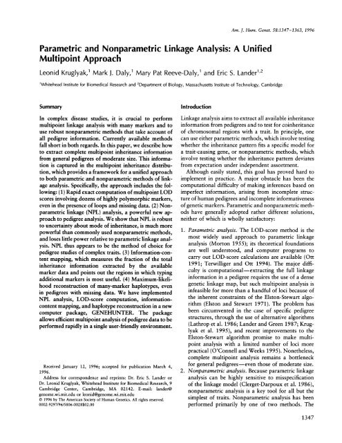
<strong>Parametric</strong> <strong>and</strong> <strong>Nonparametric</strong> <strong>Linkage</strong> <strong>Analysis</strong>: A Unified<br />
Multipoint Approach<br />
Leonid Kruglyak,' Mark J. Daly,' Mary Pat Reeve-Daly,' <strong>and</strong> Eric S. L<strong>and</strong>er',2<br />
Am. J. Hum. Genet. 58:1347-1363, 1996<br />
'Whitehead Institute for Biomedical Research <strong>and</strong> 2Department of Biology, Massachusetts Institute of Technology, Cambridge<br />
Summary Introduction<br />
In complex disease studies, it is crucial to perform<br />
multipoint linkage analysis with many markers <strong>and</strong> to<br />
use robust nonparametric methods that take account of<br />
all pedigree information. Currently available methods<br />
fall short in both regards. In this paper, we describe how<br />
to extract complete multipoint inheritance information<br />
from general pedigrees of moderate size. This information<br />
is captured in the multipoint inheritance distribution,<br />
which provides a framework for a unified approach<br />
to both parametric <strong>and</strong> nonparametric methods of linkage<br />
analysis. Specifically, the approach includes the following:<br />
(1) Rapid exact computation of multipoint LOD<br />
scores involving dozens of highly polymorphic markers,<br />
even in the presence of loops <strong>and</strong> missing data. (2) <strong>Nonparametric</strong><br />
linkage (NPL) analysis, a powerful new approach<br />
to pedigree analysis. We show that NPL is robust<br />
to uncertainty about mode of inheritance, is much more<br />
powerful than commonly used nonparametric methods,<br />
<strong>and</strong> loses little power relative to parametric linkage analysis.<br />
NPL thus appears to be the method of choice for<br />
pedigree studies of complex traits. (3) Information-content<br />
mapping, which measures the fraction of the total<br />
inheritance information extracted by the available<br />
marker data <strong>and</strong> points out the regions in which typing<br />
additional markers is most useful. (4) Maximum-likelihood<br />
reconstruction of many-marker haplotypes, even<br />
in pedigrees with missing data. We have implemented<br />
NPL analysis, LOD-score computation, informationcontent<br />
mapping, <strong>and</strong> haplotype reconstruction in a new<br />
computer package, GENEHUNTER. The package<br />
allows efficient multipoint analysis of pedigree data to be<br />
performed rapidly in a single user-friendly environment.<br />
Received January 12, 1996; accepted for publication March 4,<br />
1996.<br />
Address for correspondence <strong>and</strong> reprints: Dr. Eric S. L<strong>and</strong>er or<br />
Dr. Leonid Kruglyak, Whitehead Institute for Biomedical Research, 9<br />
Cambridge Center, Cambridge, MA 02142. E-mail: l<strong>and</strong>er@<br />
genome.wi.mit.edu or leonid@genome.wi.mit.edu<br />
© 1996 by The American Society of Human Genetics. All rights reserved.<br />
0002-9297/96/5806-0028$02.00<br />
<strong>Linkage</strong> analysis aims to extract all available inheritance<br />
information from pedigrees <strong>and</strong> to test for coinheritance<br />
of chromosomal regions with a trait. In principle, one<br />
can use either parametric methods, which involve testing<br />
whether the inheritance pattern fits a specific model for<br />
a trait-causing gene, or nonparametric methods, which<br />
involve testing whether the inheritance pattern deviates<br />
from expectation under independent assortment.<br />
Although easily stated, this goal has proved hard to<br />
implement in practice. A major obstacle has been the<br />
computational difficulty of making inferences based on<br />
imperfect information, arising from incomplete structure<br />
of human pedigrees <strong>and</strong> incomplete informativeness<br />
of genetic markers. <strong>Parametric</strong> <strong>and</strong> nonparametric methods<br />
have generally adopted rather different solutions,<br />
neither of which is wholly satisfactory:<br />
1. <strong>Parametric</strong> analysis. The LOD-score method is the<br />
most widely used approach to parametric linkage<br />
analysis (Morton 1955); its theoretical foundations<br />
are well understood, <strong>and</strong> computer programs to<br />
carry out LOD-score calculations are available (Ott<br />
1991; Terwilliger <strong>and</strong> Ott 1994). The major difficulty<br />
is computational-extracting the full linkage<br />
information in a pedigree requires the use of a dense<br />
genetic linkage map, but such multipoint analysis is<br />
infeasible for more than a h<strong>and</strong>ful of loci because of<br />
the inherent constraints of the Elston-Stewart algorithm<br />
(Elston <strong>and</strong> Stewart 1971). The problem has<br />
been circumvented in the case of specific pedigree<br />
structures, through the use of alternative algorithms<br />
(Lathrop et al. 1986; L<strong>and</strong>er <strong>and</strong> Green 1987; Kruglyak<br />
et al. 1995), <strong>and</strong> recent improvements to the<br />
Elston-Stewart algorithm promise to make multipoint<br />
analysis with a limited number of loci more<br />
practical (O'Connell <strong>and</strong> Weeks 1995). Nonetheless,<br />
complete multipoint analysis remains a bottleneck<br />
for general pedigrees-even those of moderate size.<br />
2. <strong>Nonparametric</strong> analysis. Because parametric linkage<br />
analysis can be highly sensitive to misspecification<br />
of the linkage model (Clerget-Darpoux et al. 1986),<br />
nonparametric analysis is a key tool for all but the<br />
simplest of traits. <strong>Nonparametric</strong> analysis has been<br />
performed primarily by one of two methods. The<br />
1347
1348<br />
first approach is to break pedigrees into nuclear families<br />
<strong>and</strong> apply sib-pair analysis; this is inefficient because<br />
it wastes a great deal of inheritance information<br />
contained in pedigree structure. To partly utilize<br />
pedigree information, Weeks <strong>and</strong> Lange (1988,<br />
1992) developed the affected-pedigree-member<br />
method (APM). APM is not a true linkage method.<br />
It sidesteps the thorny issue of tracing the inheritance<br />
pattern in a pedigree by focusing on whether affected<br />
relatives happen to show the same alleles at a locus<br />
(i.e., identity/identical by state [IBS]), regardless of<br />
whether the allele is actually inherited from a common<br />
ancestor (i.e., identity/identical by descent<br />
[IBD]). The extent of IBS sharing among all pairs of<br />
affected members of the pedigree is compared with<br />
Mendelian expectation under the hypothesis of no<br />
linkage. The APM approach has several drawbacks:<br />
(i) It focuses only on IBS information <strong>and</strong> ignores<br />
genotype information for additional members of the<br />
pedigree, even when this information can be used to<br />
resolve whether shared alleles are actually IBD. (ii)<br />
It involves comparisons only among pairs of individuals,<br />
which can be less powerful than tests based on<br />
larger sets of affected individuals (Whittemore <strong>and</strong><br />
Halpern 1994a; also, see below). (iii) It lacks a true<br />
multipoint formulation. Multilocus APM simply<br />
adds together statistics from several marker loci<br />
(Weeks <strong>and</strong> Lange 1992), rather than extracting linkage<br />
information about any given point. It thus tests<br />
for linkage to an extended chromosomal region<br />
rather than to a point, <strong>and</strong> therefore it cannot be<br />
used to localize a particular locus relative to a map<br />
markers. By failing to extract the full inheritance information,<br />
APM is potentially prone to false-positive<br />
<strong>and</strong> false-negative results.<br />
To avoid these inherent problems of IBS-based methods,<br />
Curtis <strong>and</strong> Sham (1994) have recently proposed an<br />
approach, called extended relative pair analysis (ERPA),<br />
that uses the risk-calculation facility of the LINKAGE<br />
package (Lathrop et al. 1984) to compute IBD-sharing<br />
probabilities for all pairs of affected individuals in a<br />
pedigree. ERPA is thus a true linkage approach to nonparametric<br />
analysis. It is limited, however, in several<br />
key respects: the comparisons are inherently confined to<br />
relative pairs; the statistical test for linkage is ad hoc;<br />
<strong>and</strong> the method cannot h<strong>and</strong>le large numbers of loci,<br />
because of the basic algorithm used in the LINKAGE<br />
package. Other approaches to nonparametric analysis<br />
have also been described (e.g., by Curtis <strong>and</strong> Sham<br />
1995).<br />
The purpose of this paper is to describe a unified<br />
approach to both parametric analysis <strong>and</strong> nonparametric<br />
analysis. The key is to separate two issues: (1) extracting<br />
information about the inheritance pattern in a<br />
Am. J. Hum. Genet. 58:1347-1363, 1996<br />
pedigree (which depends only on the genetic markers)<br />
<strong>and</strong> (2) defining a statistic to assess linkage for a given<br />
inheritance pattern (which depends only on the nature<br />
of the trait).<br />
This approach generalizes our recent methods for<br />
complete multipoint sib-pair analysis (Kruglyak <strong>and</strong><br />
L<strong>and</strong>er 1995) to the situation of arbitrary pedigrees.<br />
The generalization required the development of a new<br />
linkage algorithm for arbitrary pedigrees, as well as the<br />
definition of new statistics for performing nonparametric<br />
analysis.<br />
The paper is organized in four parts. First, we discuss<br />
how to extract all available inheritance information<br />
from a pedigree. Specifically, we present a complete<br />
multipoint algorithm for determining the probability<br />
distribution over possible inheritance patterns at each<br />
point in the genome. Second, we apply these concepts<br />
to define a unified multipoint framework for both parametric<br />
<strong>and</strong> nonparametric analysis. In the former case,<br />
the approach provides a rapid multipoint linkage algorithm<br />
for traditional LOD-score calculations. In the latter<br />
case, it provides a powerful new approach to pedigree<br />
analysis, which we refer to as nonparametric<br />
linkage (NPL) analysis. Third, we evaluate the power of<br />
NPL analysis in applications to both simulated <strong>and</strong> actual<br />
data. In all cases examined, NPL analysis is considerably<br />
more powerful than APM. Finally, we show how<br />
the framework presented here also allows reconstruction<br />
of haplotypes in pedigrees.<br />
We have implemented these methods in a computer<br />
program, GENEHUNTER, for both parametric <strong>and</strong><br />
nonparametric analysis. With current workstations, the<br />
program can rapidly analyze moderately sized pedigrees<br />
of the sort used in genetic studies of complex traits.<br />
Definitions<br />
Given a pedigree, we define nonfounders to be those<br />
individuals whose parents are in the pedigree. Without<br />
loss of generality, we will assume that pedigrees are defined<br />
to include both parents of any individual who has<br />
a sib, half-sib, or parent in the pedigree. (If such parents<br />
are unavailable for study, they are simply included in<br />
the pedigree with unknown phenotypic <strong>and</strong> genotypic<br />
status). Individuals whose parents are not in the pedigree<br />
are designated as founders. Throughout, n will denote<br />
the number of nonfounders, <strong>and</strong> f the number of founders,<br />
in a pedigree. Founders will be assumed to be unrelated;<br />
that is, they are assumed to carry 2f alleles that<br />
are distinct by descent (although some may be IBS).<br />
Representing <strong>and</strong> Computing Inheritance Information<br />
The Inheritance Vector<br />
<strong>Linkage</strong> analysis can be divided into two steps: (i)<br />
inferring information about the inheritance pattern of a
Kruglyak et al.: <strong>Parametric</strong> <strong>and</strong> <strong>Nonparametric</strong> <strong>Linkage</strong> <strong>Analysis</strong><br />
pedigree <strong>and</strong> (ii) deciding whether the inheritance information<br />
indicates the presence of a trait-causing gene.<br />
Ideally, one would like to know the precise inheritance<br />
pattern at every locus in the genome. The inheritance<br />
pattern at each point x is completely described by a<br />
binary inheritance vector v(x) = (plml Pp2,m2,<br />
... ,pn ,mn), whose coordinates describe the outcome of<br />
the paternal <strong>and</strong> maternal meioses giving rise to the n<br />
nonfounders in the pedigree (L<strong>and</strong>er <strong>and</strong> Green 1987).<br />
Specifically, pi = 0 or 1, according to whether the gr<strong>and</strong>paternal<br />
or gr<strong>and</strong>maternal allele was transmitted in the<br />
paternal meiosis giving rise to the ith nonfounder; mi<br />
carries the same information for the corresponding maternal<br />
meiosis. Thus, the inheritance vector completely<br />
specifies which of the 2f distinct founder alleles are inherited<br />
by each nonfounder. The notion of the inheritance<br />
vector is illustrated in figure 1A. The set of all 22n<br />
possible inheritance vectors will be denoted V. Similar<br />
representations of inheritance have been proposed in<br />
the context of Monte Carlo linkage analysis (Sobel <strong>and</strong><br />
Lange 1993; Thompson 1994), as well as in other applications<br />
(Whittemore <strong>and</strong> Halpern 1994a, 1994b; Guo<br />
1995).<br />
The Inheritance Distribution<br />
In practice, it is not feasible to determine the true<br />
inheritance vector at every point in the genome, since<br />
this would require genotyping all pedigree members<br />
with an infinitely dense map of fully informative markers.<br />
Because key pedigree members are frequently unavailable<br />
<strong>and</strong> genetic markers have limited heterozygosity,<br />
genotype data will provide only partial information<br />
about inheritance.<br />
Partial information extracted from a pedigree can be<br />
represented by a probability distribution over the possible<br />
inheritance vectors at each locus in the genomethat<br />
is, P(v(x) = w) for all inheritance vectors wE V. In<br />
the absence of any genotype information, all inheritance<br />
vectors are equally likely according to Mendel's first<br />
law, <strong>and</strong> the probability distribution is uniform (abbreviated<br />
as Puniform). As genotype information is added,<br />
the probability distribution is concentrated on certain<br />
inheritance vectors. The probability distribution over<br />
possible inheritance vectors will be referred to as the<br />
inheritance distribution; the notion is illustrated in figure<br />
1B <strong>and</strong> C.<br />
Calculating the Inheritance Distribution by Use of<br />
Hidden Markov Models (HMMs)<br />
To extract the full information from a data set, one<br />
must calculate the inheritance distribution conditional<br />
on the genotypes at all marker loci (abbreviated<br />
Pcomplete). L<strong>and</strong>er <strong>and</strong> Green (1987) described how, in<br />
principle, an HMM can be used to solve this problem.<br />
In brief, the approach considers the inheritance pattern<br />
a<br />
A.<br />
C.<br />
[xl,x2] [x3,x4]<br />
[xl,x3] [x5,x6]<br />
inheritance vector<br />
0000<br />
0001<br />
0010<br />
0011<br />
0100<br />
0101<br />
0110<br />
0111<br />
1000<br />
1001<br />
1010<br />
1011<br />
1100<br />
1101<br />
1110<br />
1111<br />
[xl ,x5] 5<br />
prior<br />
1/16<br />
1/16<br />
1/16<br />
1/16<br />
1/16<br />
1/16<br />
1/16<br />
1/16<br />
1/16<br />
1/16<br />
1/16<br />
1/16<br />
1/16<br />
1/16<br />
1/16<br />
1/16<br />
posterior<br />
1/8<br />
1/8<br />
0<br />
0<br />
1/8<br />
1/8<br />
0<br />
0<br />
1/8<br />
1/8<br />
0<br />
0<br />
1/8<br />
1/8<br />
0<br />
0<br />
B.<br />
AB AC<br />
true<br />
1<br />
0<br />
0<br />
0<br />
0<br />
0<br />
0<br />
0<br />
0<br />
0<br />
0<br />
0<br />
0<br />
0<br />
0<br />
0<br />
AC3 BB<br />
AB 5<br />
1349<br />
Figure 1 Illustration of the inheritance vector <strong>and</strong> its distribution,<br />
for a simple pedigree. A, Pedigree shown with individuals labeled<br />
"1" through "5." The distinct-by-descent founder alleles are labeled<br />
"xl" through "x6"; they are assumed to be phase known, with the<br />
paternally derived allele listed first. The four meiotic events whose<br />
outcomes determine inheritance in the pedigree are indicated by<br />
arrows; the labels correspond to the coordinates in the inheritance<br />
vector. The inheritance outcome shown is specified by inheritance<br />
vector (0,0,0,0)-that is, the paternally derived allele is transmitted<br />
in every meiosis. B, Same pedigree, now shown with actual genotypes<br />
at a marker with three alleles, A, B, <strong>and</strong> C. Only the outcome of<br />
meiosis 3 is unambiguously determined by the genotype data-the<br />
paternally derived allele is transmitted, fixing the third bit in the inheritance<br />
vector at 0. C, Inheritance distribution for the 16 possible inheritance<br />
vectors. "prior" denotes distribution before any genotyping has<br />
been performed; "posterior" denotes distribution based on genotypes<br />
in panel B; <strong>and</strong> "true" denotes distribution based on fully informative,<br />
phase-known genotypes as in panel A.<br />
across the genome as a Markov process (with recombination<br />
causing transitions among states) that is observed,<br />
imperfectly, only at marker loci. One uses the<br />
imperfect observations at each marker (more precisely,<br />
the probability distribution over inheritance vectors at<br />
each marker locus, conditional only on the data for the<br />
locus itself [abbreviated as Pmarker]), to reconstruct the<br />
probability distribution at any point, conditional on the<br />
entire data set, according to the st<strong>and</strong>ard forward-backward<br />
conditioning approach employed in HMMs (Rabiner<br />
1989). In the basic L<strong>and</strong>er-Green algorithm, the time<br />
-
1350<br />
required for the HMM reconstruction step with m markers<br />
is O(m 2"). Because this scales linearly with the<br />
number of loci but exponentially with the number of<br />
nonfounders, the approach is best suited to complete<br />
multipoint analyses in pedigrees of moderate size. In<br />
contrast, the Elston-Stewart algorithm scales exponentially<br />
with loci but linearly with nonfounders <strong>and</strong> thus<br />
is best suited for studying one or a few markers in large<br />
pedigrees.<br />
First Speedup<br />
Kruglyak et al. (1995) recently showed how to decrease<br />
the time required for the HMM reconstruction<br />
step from O(m * 2") to O(m * n22n), thereby effectively<br />
doubling the pedigree size to which the HMM approach<br />
can be applied. With this speedup, the approach has<br />
been implemented in special cases, to allow complete<br />
multipoint analysis for homozygosity mapping, linkage<br />
analysis in nuclear families, <strong>and</strong> sib-pair analysis (Kruglyak<br />
et al. 1995; Kruglyak <strong>and</strong> L<strong>and</strong>er 1995). To apply<br />
the approach to general pedigrees, it is necessary to have<br />
an algorithm for calculating the initial distributions used<br />
in the HMM, Pmarker for pedigrees of arbitrary structure.<br />
We have now devised such an algorithm, which is described<br />
in appendix A.<br />
Second Speedup<br />
We have devised a further substantial acceleration of<br />
the HMM, by taking advantage of a certain degeneracy<br />
among the inheritance vectors. Since a pedigree contains<br />
no information about founder phase, inheritance vectors<br />
that differ only by phase changes in the founders are<br />
completely equivalent <strong>and</strong> must therefore have equal<br />
probabilities. In a pedigree with f founders, the inheritance<br />
vectors can thus be organized into equivalence<br />
classes consisting of 2f equivalent members. The HMM<br />
algorithm can be modified to work with just a single<br />
representative from each equivalence class, as described<br />
in appendix B. This reduces both the time <strong>and</strong> space<br />
requirements of the calculation by a factor of 2f, further<br />
increasing the size of pedigrees that may be analyzed.<br />
The running time for analysis of m markers is thus<br />
- O(m n22-f )<br />
Computer Implementation<br />
We have implemented the HMM approach with these<br />
two speedups in a new computer package, GENE-<br />
HUNTER. On current workstations, GENEHUNTER<br />
can comfortably h<strong>and</strong>le pedigrees with 2n - f -<br />
16,<br />
or, typically, approximately a dozen nonfounders. Some<br />
examples of pedigrees that can be readily analyzed are<br />
given in figure 2.<br />
The same methods also can be used to estimate the<br />
number of recombination events between two markers.<br />
GENEHUNTER includes an option to compute this<br />
A<br />
B<br />
C<br />
Am. J. Hum. Genet. 58:1347-1363, 1996<br />
OIT-*2<br />
25 26<br />
30 31 0 41 42<br />
Figure 2 Examples of pedigrees that can be analyzed by using<br />
GENEHUNTER. A, Simple three-generation pedigree segregating a<br />
dominant disorder. Individuals in the last two generations are available<br />
for study. B, Complex inbred pedigree that occurred in the study<br />
of Werner syndrome (Thompson <strong>and</strong> Wijsman 1994). Only the affected<br />
individual in the last generation is available for study. C, Pedigree<br />
with three affected fourth cousins. Only the affected individuals<br />
in the last generation are available for study.<br />
number for pairs of consecutive markers, which can be<br />
useful for detecting genotyping errors that cause map<br />
inflation.<br />
Information-Content Mapping<br />
In studying a pedigree, it is useful to know how much<br />
of the total inheritance information has been extracted
Kruglyak et al.: <strong>Parametric</strong> <strong>and</strong> <strong>Nonparametric</strong> <strong>Linkage</strong> <strong>Analysis</strong><br />
at each point in the genome, given the available genotype<br />
data. We introduced a notion of "information-content<br />
mapping" in our previous work on sib-pair analysis<br />
(Kruglyak <strong>and</strong> L<strong>and</strong>er 1995). Information content provides<br />
a measure of how closely a study approaches the<br />
goal of completely determining the inheritance outcome,<br />
<strong>and</strong> it points out the regions where typing additional<br />
markers is most useful. Here, we modify our previous<br />
approach <strong>and</strong> extend it to arbitrary pedigrees.<br />
The classical information-theoretic measure of residual<br />
uncertainty in a probability distribution is its entropy,<br />
defined by E = -IPilog2Pi, where Pi is the probability<br />
of the ith outcome <strong>and</strong> where log2 is used in order<br />
for the entropy to be measured in bits (Shannon 1948).<br />
The entropy of the probability distribution over inheritance<br />
vectors thus naturally reflects information content.<br />
In the absence of genotype data, the probability distribution<br />
is uniform over all 22n-f equivalence classes of<br />
inheritance vectors. The entropy of the distribution is<br />
easily seen to be E = 2n - f bits. This result makes<br />
intuitive sense, since we are completely uncertain about<br />
the outcome of the 2n - fmeioses for which information<br />
can be obtained. If the inheritance vector is known with<br />
certainty (e.g., at a fully informative marker), the probability<br />
distribution is completely concentrated on a single<br />
outcome. The entropy is thus E = 0, which again makes<br />
intuitive sense.<br />
The information content of the inheritance pattern at<br />
point x will be defined by<br />
IE(X) = 1 - E(x)/Eo, (1)<br />
where E(x) is the entropy of the multipoint inheritance<br />
distribution at x <strong>and</strong> where Eo = 2n - f bits is the<br />
entropy in the absence of genotype data. Information<br />
content IE(X) = 1 indicates perfect informativeness at x,<br />
whereas information content IE(X) = 0 indicates total<br />
uncertainty about inheritance in the pedigree at x. Since<br />
entropy is an additive measure, it can be summed over<br />
all pedigrees in the data set. Equation (1) is then used<br />
with total entropy to obtain the overall information content<br />
of a study.<br />
IE is a general measure of information content. It does<br />
not depend on any particular test for linkage <strong>and</strong> has<br />
the desirable property that it always lies between 0 <strong>and</strong><br />
1. (This contrasts with a somewhat different measure of<br />
information content, which we discussed in previous<br />
work on sib-pair analysis [Kruglyak <strong>and</strong> L<strong>and</strong>er 1995].)<br />
An example of information content for different map<br />
densities is shown in figure 3.<br />
Unified <strong>Linkage</strong> <strong>Analysis</strong><br />
We now define both parametric <strong>and</strong> nonparametric<br />
analysis from a unified perspective, which is based on<br />
c<br />
u<br />
0<br />
(a<br />
Chromosome position (cM)<br />
Figure 3 Information-content mapping for various marker densities.<br />
Genotypes for markers spaced every 2 cM on a 100-cM map,<br />
with typical microsatellite informativeness levels (heterogeneity .75),<br />
were simulated for 10 sibships having four sibs each, with missing<br />
parents. The five curves show the information content with markers<br />
genotyped at SO-cM, 25-cM, 12-cM, 6-cM, <strong>and</strong> 2-cM average spacing<br />
(corresponding, respectively, to 3, 5, 9, 17, <strong>and</strong> 51 markers genotyped<br />
across the map). The average information content increases from<br />
-40% to 54%, 63%, 72%, <strong>and</strong> 85%, respectively.<br />
the notion of inheritance vectors. In the ideal situationthe<br />
precise inheritance vector v(x) at each point x is<br />
known with certainty-linkage analysis simply involves<br />
quantifying the extent to which the inheritance vector<br />
indicates the presence of a disease gene. This can be done<br />
by specifying a scoring function S(vA)) that depends on<br />
the inheritance vector v <strong>and</strong> the observed phenotypes 1<br />
in the pedigree.<br />
To extend the analysis to the more realistic situation<br />
in which one has only a probability distribution over<br />
v(x), one can generalize the scoring function by taking<br />
its expected value over the inheritance distribution:<br />
S(xA) = I S(w,$)P[v(x) = w].<br />
wEV<br />
Given the probability distribution over inheritance vectors<br />
at every point x, it is then straightforward to calculate<br />
S throughout the genome. Specifically, one could<br />
calculate once <strong>and</strong> store the 22n-f values of S(vA). For<br />
each point x, one could then compute the linear combination<br />
in equation (2) in time 0(22n-f ). We now consider<br />
various choices of scoring functions S that correspond<br />
to parametric linkage analysis <strong>and</strong> NPL analysis.<br />
<strong>Parametric</strong> <strong>Linkage</strong> <strong>Analysis</strong><br />
1351<br />
Scoring Function<br />
In parametric linkage analysis, one assumes a model<br />
describing the probability of phenotype given genotype<br />
(2)
1352<br />
at the disease locus <strong>and</strong> calculates the likelihood ratio<br />
under the hypothesis that a disease gene is at x, versus<br />
the hypothesis that it is unlinked to x. In the special<br />
case when the inheritance vector is known, the scoring<br />
function S is simply the likelihood ratio. It is given by<br />
LR(v) = P(( I v)<br />
E P((F W)Puniform(W)<br />
wE- V<br />
P((D v) is simply the likelihood of observed phenotypes<br />
(D, conditioned on the particular inheritance vector v; it<br />
depends only on the penetrance values <strong>and</strong> allele frequencies<br />
at the disease locus. For each v, one can efficiently<br />
compute P((D v) by a simple adaptation of st<strong>and</strong>ard<br />
peeling methods for pedigrees without loops<br />
(Elston <strong>and</strong> Stewart 1971; Lange <strong>and</strong> Elston 1975; Cannings<br />
et al. 1978; Whittemore <strong>and</strong> Halpern 1994b) <strong>and</strong><br />
by a combination of peeling, loop breaking, <strong>and</strong> enumeration<br />
of founder genotypes for pedigrees with loops (for<br />
details, see appendix C). Calculating the likelihood for<br />
each of the 22n-f equivalence classes of inheritance vectors<br />
is rapid for moderate-sized pedigrees, both with <strong>and</strong><br />
without loops.<br />
In the general case, we take the expectation of the<br />
scoring function over the inheritance distribution, as in<br />
equation (2):<br />
LR(x) = A LR(w)P(v(x) = w)<br />
we V<br />
I P(4) W)Pcomplete(W)<br />
= wEV<br />
I P(F W)Puniform(W)<br />
wEV<br />
This expression is easily seen to be equivalent to the<br />
traditional definition of the likelihood ratio-the numerator<br />
is proportional to the multipoint likelihood<br />
when the disease gene is at x, whereas the denominator<br />
is proportional to the unlinked likelihood. According to<br />
long-st<strong>and</strong>ing tradition, one reports the LOD score,<br />
loglo(LR).<br />
Because traditional LOD-score analysis can be expressed<br />
in the unified framework above, the fast HMM<br />
approach provides a rapid algorithm for performing<br />
complete multipoint linkage analysis in moderate-sized<br />
pedigrees. The LOD scores obtained by this method are<br />
exact-no approximations are involved. The only difference<br />
with conventional algorithms is the speed of<br />
computation when many markers are considered simultaneously.<br />
Implementation<br />
We have implemented parametric linkage analysis<br />
within GENEHUNTER. The program can compute<br />
LOD scores for arbitrary pedigrees under particular<br />
Am. J. Hum. Genet. 58:1347-1363, 1996<br />
models of inheritance, allowing the user to specify allele<br />
frequencies at the disease locus <strong>and</strong> penetrances for liability<br />
classes (including age- <strong>and</strong> sex-dependent penetrances).<br />
The program also allows the user to test for<br />
linkage under genetic heterogeneity by using an admixture<br />
model (Ott 1991; Terwilliger <strong>and</strong> Ott 1994) to estimate<br />
the proportion of linked families a. Alternatively,<br />
the user can specify the admixture parameter a.<br />
To illustrate its performance, GENEHUNTER was<br />
applied to simulated data for the pedigrees shown in<br />
figure 2. For each pedigree, we simulated genotype data<br />
for a genetic map of 20 markers under the hypothesis<br />
of a disease-causing gene located in the middle of the<br />
map. We then calculated complete multipoint LOD<br />
scores at each marker <strong>and</strong> at four points within each<br />
interval between markers, that is, at 96 distinct map<br />
locations (fig. 4). On a DEC Alpha workstation, the<br />
computation times for these 96 21-point LOD scores<br />
(disease locus plus all 20 markers) were 24 min, 82 min,<br />
<strong>and</strong> 280 min, for pedigrees A, B. <strong>and</strong> C, respectively.<br />
(The respective values of 2n - f are 14, 15, <strong>and</strong> 16).<br />
For each of the three pedigrees, the maximum LOD<br />
score computed by using complete multipoint analysis<br />
approaches the theoretical maximum LOD score that<br />
would be obtained with an infinitely polymorphic<br />
marker located at a recombination fraction of zero from<br />
the disease gene. In particular, for pedigree C in figure<br />
2, the three isolated fourth cousins have a probability of<br />
( 1/2)13 of sharing an allele IBD, resulting in a theoretical<br />
maximum LOD score of 3.91. The multipoint LOD<br />
score nearly achieves this maximum, with a LOD of<br />
3.84 (fig. 4C), indicating that it has extracted essentially<br />
all inheritance information. In contrast, the maximum<br />
LOD score attainable with a single marker is only 1.87,<br />
<strong>and</strong> the maximum LOD score with two flanking markers<br />
is 1.98. In this case, multipoint analysis increases the<br />
LOD score from moderately interesting to significant,<br />
providing almost 100-fold-higher odds in favor of linkage<br />
than does two-point analysis.<br />
To further explore the value of multipoint analysis,<br />
we considered the simpler case of a pedigree with two<br />
affected fourth cousins <strong>and</strong> all other pedigree members<br />
unavailable for study. We once again simulated a 20marker<br />
map under the hypothesis of a linked rare dominant<br />
gene. The IBD-sharing probability for two fourth<br />
cousins is 1/256, yielding a theoretical maximum LOD<br />
score of 2.41. In figure 5, we plot the maximum LOD<br />
score achieved by analyzing k = 1, . . . ,20 consecutive<br />
markers simultaneously. Complete 20-marker analysis<br />
yields a LOD score of 2.2 (91% of theoretical maximum).<br />
In contrast, the highest two-point LOD score<br />
is only 0.83 (34% of theoretical maximum), <strong>and</strong> even<br />
simultaneous six-marker analysis yields, at most, a LOD<br />
score of 1.74 (72% of theoretical maximum). These results<br />
underscore the value that multipoint analysis with
Kruglyak et al.: <strong>Parametric</strong> <strong>and</strong> <strong>Nonparametric</strong> <strong>Linkage</strong> <strong>Analysis</strong><br />
(M<br />
0<br />
0<br />
0<br />
A<br />
0 w<br />
'0 0<br />
-J la<br />
ao<br />
B<br />
Map position (cM) Map position (cM) Map position (cM)<br />
Figure 4 Multipoint LOD-score plots for the pedigrees shown in figure 2. Genotypes for 20 markers were simulated under the assumption<br />
of a disease gene at the location indicated by an arrow. A total of 96 21-point LOD scores were computed, with the disease locus tested at<br />
each marker <strong>and</strong> at four evenly spaced locations in each interval between markers. Marker positions are indicated by tick marks on the<br />
horizontal axis. A, Pedigree of figure 2A, with a rare dominant gene (frequency 10-4). B, Pedigree of figure 2B, with a rare recessive gene<br />
(frequency 10-4). C, Pedigree of figure 2C, with a very rare dominant gene (frequency 10-6).<br />
many markers has for extracting the full inheritance<br />
information. Such multipoint analysis is clearly desirable,<br />
since it requires only 40 s on a SUN SPARC workstation<br />
running GENEHUNTER.<br />
To compare the performance of GENEHUNTER with<br />
that of other linkage packages, we analyzed the pedigree<br />
with two affected fourth cousins, using FASTLINK<br />
(Cottingham et al. 1993) <strong>and</strong> VITESSE (O'Connell <strong>and</strong><br />
Weeks 1995), both running on a SUN SPARC workstation.<br />
FASTLINK required 32 min to compute LOD<br />
scores when using overlapping sets of two markers (28<br />
three-point calculations), with a maximum LOD score<br />
of 0.98. Four-point calculations failed to complete after<br />
-1-00 h. VITESSE required 85 s to compute LOD scores<br />
when using two markers simultaneously, 30 min to compute<br />
LOD scores when using three markers simultaneously<br />
(54 four-point calculations; maximum LOD score<br />
of 1.28), <strong>and</strong> 19 h 14 min to compute lod scores when<br />
using four markers simultaneously (68 five-point calculations;<br />
maximum LOD score of 1.43). Six-point calculations<br />
failed to complete after '100 h. These other<br />
programs thus can perform multipoint analysis with a<br />
h<strong>and</strong>ful of markers, but not the complete multipoint<br />
calculations necessary to extract all available inheritance<br />
information. On the other h<strong>and</strong>, these programs are able<br />
to h<strong>and</strong>le very large pedigrees that are beyond the computational<br />
limitations of GENEHUNTER.<br />
GENEHUNTER's speed is independent of the number<br />
of alleles per marker (thereby allowing highly polymorphic<br />
markers to be used without recoding) <strong>and</strong> is essentially<br />
independent of the amount of missing information<br />
in the pedigree. The program has been tested extensively<br />
a)<br />
0 n<br />
U,<br />
'0 0<br />
-..<br />
C<br />
by comparing the results with those produced by LINK-<br />
AGE (Lathrop et al. 1984) <strong>and</strong> FASTLINK (Cottingham<br />
et al. 1993), for a variety of family structures <strong>and</strong> modes<br />
of inheritance (in analyses using a small number of<br />
markers). In all case examined, the three programs produced<br />
identical answers.<br />
NPL <strong>Analysis</strong><br />
1353<br />
Scoring Functions<br />
We begin by considering the special case in which the<br />
inheritance vector is known with certainty. The inheritance<br />
vector fully determines which of the 2f distinct<br />
founder alleles was inherited by each person <strong>and</strong> thus<br />
completely specifies IBD sharing in the pedigree. The<br />
only issue is to define a suitable scoring function to<br />
measure whether affected individuals share alleles IBD<br />
more often than expected under r<strong>and</strong>om segregation.<br />
One simple approach would be to assign a score of 1 if<br />
all affected individuals in a pedigree share an allele IBD<br />
<strong>and</strong> to assign a score of 0 otherwise (Thomas et al.<br />
1994). However, this statistic is likely not to be robust<br />
in the presence of phenocopies <strong>and</strong> common disease alleles.<br />
We consider below two useful scoring functions,<br />
Spairs <strong>and</strong> Sall, previously discussed by Whittemore <strong>and</strong><br />
Halpern (1994a); other scoring functions can be defined.<br />
1. IBD sharing in pairs.-One possible approach is to<br />
count pairwise allele sharing among affected relatives.<br />
Given the inheritance vector v, Spairs(v) is defined to be<br />
the number of pairs of alleles from distinct affected pedigree<br />
members that are IBD. The traditional APM statistic<br />
(Weeks <strong>and</strong> Lange 1988) also counts pairwise allele
1354<br />
I-<br />
0<br />
0<br />
2-<br />
I<br />
..s.............................................................................................<br />
0<br />
0<br />
0<br />
00<br />
0<br />
*0<br />
t i-I- . .<br />
0 5 10 15 20<br />
Marker number<br />
Figure 5 Maximum LOD score achieved in a pedigree with two<br />
affected fourth cousins, plotted as a function of k, the number of<br />
markers analyzed simultaneously. Genotypes for 20 markers were<br />
simulated by assuming the presence of a very rare dominant disease<br />
gene (frequency 10-6) in the middle of an 18-cM map, as in figure<br />
4C. LOD scores were computed with the disease locus tested at the<br />
markers <strong>and</strong> at four points within each interval between markers;<br />
genotype data from overlapping sets of k consecutive markers were<br />
used. Black dots show results for multipoint analysis with sets of<br />
1,2,3,. . . ,11, <strong>and</strong> 20 markers; <strong>and</strong> the dotted line shows the theoretical<br />
maximum LOD score of 2.41 for this pedigree. The maximum<br />
LOD score of 2.2, achieved with 20 markers, is the highest possible<br />
with this marker density <strong>and</strong> polymorphism; doubling the marker<br />
density <strong>and</strong> performing multipoint analysis with 40 markers raises the<br />
maximum LOD score to 2.4 (data not shown).<br />
sharing, but it is based on sharing IBS rather than on<br />
sharing IBD; the two statistics will coincide only at<br />
markers for which IBS unambiguously determines IBD.<br />
2. IBD sharing in larger sets.-One can often increase<br />
statistical power by considering larger sets of affected<br />
relatives, rather than just pairs. For example, it is more<br />
impressive to find that five affected relatives share the<br />
same allele IBD than to find that each pair of them shares<br />
some allele IBD. Whittemore <strong>and</strong> Halpern (1994a) proposed<br />
an interesting statistic to capture the allele sharing<br />
associated with a given inheritance vector v. Let a denote<br />
the number of affected individuals in the pedigree, let h<br />
be a collection of alleles obtained by choosing one allele<br />
from each of these affected individuals, <strong>and</strong> let bi(h)<br />
denote the number of times that the ith founder allele<br />
appears in h (for i = 1, . .. ,2f). The score Sall is defined<br />
as<br />
Sali(V) = 2 a L[ bi(h)!1<br />
h i= 1<br />
where the sum is taken over the 2a possible ways to<br />
choose h. In effect, the score is the average number of<br />
4<br />
Am. J. Hum. Genet. 58:1347-1363, 1996<br />
permutations that preserve a collection obtained by<br />
choosing one allele from each affected person. It gives<br />
sharply increasing weight as the number of affected individuals<br />
sharing a particular allele increases.<br />
For either approach, we define a normalized score<br />
Z(v) = [S(v) - p1/a, (3)<br />
where J <strong>and</strong> a are the mean <strong>and</strong> SD of S under Puniform<br />
the uniform distribution over the possible inheritance<br />
vectors. (These quantities can be calculated by enumeration<br />
over all vectors.) Under the null hypothesis of no<br />
linkage (i.e., Puniform), the normalized score Z has mean<br />
0 <strong>and</strong> variance 1.<br />
To combine scores among m pedigrees, one can take<br />
a linear combination<br />
m<br />
Z= xYiZi,<br />
i=l<br />
where m is the number of pedigrees, Zi denotes the normalized<br />
score for the ith pedigree, <strong>and</strong> the y, are<br />
weighting factors. The weighting factors should be chosen<br />
so that i = 1, so that Z has mean 0 <strong>and</strong> variance<br />
1 under the null hypothesis of no linkage. We will use<br />
Yj = i1Fm in the applications below; this choice appears<br />
to provide a good compromise between small <strong>and</strong> large<br />
pedigrees. It may be possible to increase power by selecting<br />
y, according to the nature of the pedigrees, but we<br />
will not explore this issue here, other than to note that<br />
the optimal choice will likely depend on the (usually<br />
unknown) genetic architecture of particular diseases.<br />
We will refer to Z as the NPL score for the collection<br />
of pedigrees. In some cases, we will speak of NPLpairs<br />
<strong>and</strong> NPLall scores, to indicate the scoring function under<br />
consideration.<br />
Statistical Significance<br />
Suppose that analysis of pedigrees yields an NPL statistic<br />
of Zobs. What is the significance level of this observation?<br />
There are two simple approaches:<br />
1. Exact distribution. It is straightforward to compute<br />
the exact probability distribution of the overall score<br />
Z under the null hypothesis of no linkage. Specifically,<br />
one can calculate the distribution for each pedigree<br />
by enumerating all possible inheritance vectors;<br />
the distribution for the collection of pedigrees is then<br />
obtained by convolving these distributions. One can<br />
then simply look up the exact value, P(Z ' Zobs).<br />
2. Normal approximation. Under the null hypothesis<br />
of no linkage, the score Z will tend toward a st<strong>and</strong>ard<br />
normal variable as one studies many similar pedigrees.<br />
(This follows from the central limit theorem,<br />
since Z is an appropriately normalized sum of inde-<br />
(4)
Kruglyak et al.: <strong>Parametric</strong> <strong>and</strong> <strong>Nonparametric</strong> <strong>Linkage</strong> <strong>Analysis</strong><br />
pendent r<strong>and</strong>om variables.) The significance level of<br />
an observation Zobs can then be approximated by<br />
consulting a table of tail probabilities for the st<strong>and</strong>ard<br />
normal. Although less precise than the exact<br />
distribution, the normal approximation is useful in<br />
some settings.<br />
Imperfect Data<br />
We have so far considered the situation in which the<br />
inheritance vector is known with certainty. In fact, it is<br />
straightforward to extend Z to the general case, by taking<br />
its expected value over the inheritance distribution,<br />
as in equation (2): Z(x,F) = 4wev Z(wA) Prob[v(x)<br />
= w], where the probability distribution over inheritance<br />
vectors here refers to the joint distribution over<br />
all pedigrees. To be precise, for a single pedigree we<br />
replace S(v) by SKin equation (3); the normalized scores<br />
for individual pedigrees are then combined into an overall<br />
score as in equation (4).<br />
The only complication is in evaluating the statistical<br />
significance of Z. Because Z is the expectation over the<br />
observed inheritance distribution, its statistical properties<br />
depend on the distribution of possible inheritance<br />
distributions (given the markers <strong>and</strong> pedigree structure).<br />
This distribution could be explicitly studied by Monte<br />
Carlo sampling from all possible realizations of the<br />
marker data. However, it is not hard to show that Z<br />
has the following properties under the null hypothesis<br />
of no linkage (see appendix D):<br />
1.<br />
2.<br />
mean(Z) = mean(Z) = 0;<br />
variance(Z) -<br />
variance(Z) = 1;<br />
3. Z is asymptotically normally distributed as one studies<br />
a large number of similar pedigrees.<br />
Moreover, Z approaches Z as information content approaches<br />
100%, under both the null hypothesis of no<br />
linkage <strong>and</strong> the alternative hypothesis of linkage. Given<br />
these properties, it seems reasonable to evaluate the statistical<br />
significance of an observation Zobs by using the<br />
null distribution of Z expected in the case of complete<br />
informativeness. The significance level is likely to be<br />
conservative (in view of 1 <strong>and</strong> 2; eqq. [5] <strong>and</strong> [6]) <strong>and</strong><br />
becomes increasingly accurate as information content<br />
increases. We will refer to this approach as the perfectdata<br />
approximation.<br />
Simulation studies (see below) show that the perfectdata<br />
approximation is indeed conservative but that it<br />
sacrifices relatively little power except when information<br />
content is very low. Indeed, significance levels appear to<br />
be within twofold of the empirical values obtained from<br />
simulations. The approximation should thus not hamper<br />
initial detection of interesting regions <strong>and</strong> should grow<br />
I<br />
II<br />
inl<br />
Figure 6 Pedigree structure used in the power simulations. Disease<br />
inheritance was simulated for four models: dominant, recessive,<br />
<strong>and</strong> two intermediate models (for details on the models, see table 1).<br />
Pedigrees were selected for analysis if they had at least three affecteds<br />
in generation III, including at least one affected individual in each<br />
sibship. Individuals in generation I were assumed to be unavailable<br />
for genotyping. Genotypic data were simulated for 11 markers spaced<br />
every 10 cM on a 100-cM map; all markers had five equally frequent<br />
alleles (heterogeneity .8). The disease locus was assumed to lie in the<br />
middle of the map, exactly at marker 6. A total of 100 pedigrees were<br />
simulated for each model, <strong>and</strong> 100 sets of 5 or 10 pedigrees each<br />
(depending on the model; see table 1) were resampled from this initial<br />
set for power calculations.<br />
increasingly accurate as one genotypes additional markers<br />
in these regions.<br />
Implementation<br />
We have implemented the calculation of both NPLpairs<br />
<strong>and</strong> NPLall scores within GENEHUNTER. Given the<br />
inheritance distribution at each point in the genome, the<br />
calculation of NPL scores is rapid. The program reports<br />
the normalized score Zi for each pedigree, the overall<br />
statistic Z, <strong>and</strong> the significance levels for the perfectdata<br />
approximation based on the exact approach.<br />
Although we have focused only on Spairs <strong>and</strong> Sal, it is<br />
straightforward to substitute other scoring functions to<br />
include further information about sharing among affected<br />
individuals or even about nonsharing between<br />
affected individuals <strong>and</strong> unaffected individuals. Such<br />
scoring functions can be easily incorporated into GENE-<br />
HUNTER.<br />
Evaluation of NPL <strong>Analysis</strong><br />
1355<br />
Power Comparisons<br />
We compared the performance of the various linkage<br />
methods on simulated data, assuming dominant, recessive,<br />
<strong>and</strong> two intermediate models <strong>and</strong> a 10-cM genetic<br />
map with markers having heterozygosity of 80%. The<br />
pedigree structure used in the simulations is shown in<br />
figure 6 (for details, see the legend to fig. 6). The pedigrees<br />
were analyzed by using complete multipoint parametric<br />
linkage analysis (under the model used to generate<br />
the data), complete multipoint NPL analysis (using<br />
both the Spairs <strong>and</strong> Saii scoring functions), <strong>and</strong> APM analysis<br />
(Weeks <strong>and</strong> Lange 1988, 1992). The performance
13S6<br />
Table 1<br />
Power Comparisons Based on Simulations<br />
P<br />
== =<br />
Am. J. Hum. Genet. 58:1347-1363, 1996<br />
.05 .01 .001 .0001 .00001 .05 .01 .001 .0001 .00001<br />
Power to Detect <strong>Linkage</strong> with N Pedigrees Expected No. of Pedigrees Required for<br />
(%) Detection of <strong>Linkage</strong><br />
Dominant: Dominant:<br />
NPLai1 100 99 95 92 81 NPLaii 1 1 2 3 4<br />
NPLpairs 99 95 67 33 10 NPLpairs 2 3 5 7 9<br />
APM 62 42 15 5 2 APM 5 8 15 22 29<br />
LOD 100 100 100 100 100 LOD 1 1 2 2 3<br />
Recessive: Recessive:<br />
NPLall 100 99 96 79 66 NPLaii 1 2 3 3 4<br />
NPLpairs 100 100 97 82 62 NPLpairs 1 2 3 4 5<br />
APM 87 59 34 19 10 APM 2 4 6 9 11<br />
LOD 100 100 100 100 100 LOD 1 1 2 3 3<br />
Complex 1: Complex 1:<br />
NPLail 64 40 17 7 4 NPLaIj 10 20 34 50 65<br />
NPLpairs 58 25 7 1 0 NPLpairs 16 31 55 79 102<br />
APM 40 23 10 2 1 APM 21 42 74 107 141<br />
LOD 77 57 27 4 1 LOD 6 11 19 28 36<br />
Complex 2: Complex 2:<br />
NPLaii 100 99 98 92 79 NPLaii 2 3 4 6 8<br />
NPLpairs 100 99 92 71 49 NPLpairs 2 4 6 8 11<br />
APM 83 68 41 14 5 APM 4 8 14 20 26<br />
LOD 99 99 97 95 87 LOD 1 2 4 5 7<br />
NoTE.-N = S was used for the dominant <strong>and</strong> recessive models, <strong>and</strong> N = 10 was used for the two complex models. Power was defined as<br />
the number of data sets (from 100) in which the appropriate threshold was exceeded. Model parameters were as follows (fd = disease gene<br />
frequency; P++, P+d, <strong>and</strong> Pdd = penetrances of + +, +d, <strong>and</strong> dd genotypes, respectively): for the dominant model, fd = .01, p++<br />
= .001, P+d = .999, <strong>and</strong> Pdd = .999; for the recessive model, fd = .05, pI+ = .001, P+d = .001, <strong>and</strong> pdd = .999; for the complex model 1, fd =<br />
.05, P++ = .05, P+d = .4, <strong>and</strong> Pdd = .6; <strong>and</strong>, for the complex model 2, fd = .01, p++ = .01, P+d = .45, <strong>and</strong> Pdd = .75. These parameters correspond<br />
to disease incidence of 2.1%, 0.35%, 8.5%, <strong>and</strong> 1.9%, respectively, <strong>and</strong> to phenocopy rates of 5%, 29%, 53%, <strong>and</strong> 52%, respectively. The<br />
thresholds used for asymptotic significance levels of .05, .01, .001, <strong>and</strong> .0001, <strong>and</strong> .00001 were .59, 1.17, 2.07, 3.00, <strong>and</strong> 3.95, respectively, for<br />
the LOD score (LOD) <strong>and</strong> 1.65, 2.33, 3.09, 3.72, <strong>and</strong> 4.27, respectively, for the normal scores (NPL <strong>and</strong> APM). LOD scores were computed by<br />
using GENEHINTER, in order to carry out multipoint analysis with 11 markers in reasonable time. Multipoint NPL statistics <strong>and</strong> multipoint<br />
LOD scores were computed by using all 11 markers simultaneously. As noted in the text, multilocus APM does not compute a multipoint statistic<br />
as a function of location. Instead, a statistic testing linkage to a region is computed. Recombination between loci is not fully taken into account,<br />
with the result that the statistic can decrease as additional flanking markers are considered, even in the presence of linkage. Therefore, we computed<br />
single-locus APM statistics by using the marker at the true locus, as well as multilocus APM statistics including 1, 2, 3, 4, <strong>and</strong> 5 closest flanking<br />
markers on each side, <strong>and</strong> we chose the highest statistic for each replicate when estimating power.<br />
of the parametric LOD-score method under the correct<br />
model was used as a benchmark, although it should be<br />
noted that the correct model is usually unknown <strong>and</strong><br />
that model misspecification can lead to considerable loss<br />
of power.<br />
We used two criteria to assess performance: (1) the<br />
power to detect a locus in a fixed sample of pedigrees<br />
<strong>and</strong> (2) the expected number of pedigrees required to<br />
detect a locus. Both measures were completed for various<br />
nominal significance levels (p = .05, .01, .001,<br />
.0001, <strong>and</strong> .00001). The results are summarized in table<br />
1. Three main conclusions emerge.<br />
First, the NPLai statistic performed better than the<br />
NPLpairs statistic in all cases studied (except for the reces-<br />
sive case, where the two showed comparable performance).<br />
This accords with the intuition that testing<br />
whether the same allele is found IBD in many affected<br />
relatives is a more powerful strategy than considering<br />
one relative pair at a time. The NPLa,, statistic thus appears<br />
to have the desirable property of robustness, <strong>and</strong><br />
it was used in all other comparisons.<br />
Second, the NPL statistic was much more powerful<br />
than the APM statistic, for all models examined. On<br />
average, at a given significance level, NPL required two<br />
to seven times fewer pedigrees for detecting linkage. The<br />
greater power of NPL is explained by its efficient use of<br />
all available information from simultaneous consideration<br />
of both all relatives <strong>and</strong> all markers.
Kruglyak et al.: <strong>Parametric</strong> <strong>and</strong> <strong>Nonparametric</strong> <strong>Linkage</strong> <strong>Analysis</strong><br />
Table 2<br />
Empirical False-Positive Rates Observed in 50,000 Simulations<br />
FALSE-POSITIVE RATE AT P =<br />
.05 .01 .001 .0001 .00001<br />
Sall, exact .03 .004 .0003 .00002 0<br />
Sall, normal .04 .008 .001 .0002 .00006<br />
Spairs, exact .03 .005 .0004 0 0<br />
Spairs, normal .04 .008 .001 .0001 0<br />
NoTE.-Genotypes for 50,000 data sets consisting of seven small<br />
two- <strong>and</strong> three-generation pedigrees were simulated, under the assumption<br />
that there is no linked disease-causing locus. "exact" refers<br />
to p values obtained from the exact distribution of scores; <strong>and</strong> "normal"<br />
refers to p values obtained from the normal approximation. The<br />
perfect-data approximation is used in both cases.<br />
Third, the performance of NPL was roughly comparable<br />
to that of the LOD-score analysis under the correct<br />
model. NPLaI thus appears to provide a nonparametric<br />
pedigree-analysis method that loses relatively little power<br />
when compared with the best parametric method. This<br />
feature is particularly significant because the NPL method<br />
requires neither consideration of multiple models of inheritance<br />
(thus avoiding corrections for multiple testing) nor<br />
advance knowledge of the correct model of inheritance<br />
(thus avoiding problems of misspecification).<br />
In addition to the power comparisons, we also examined<br />
the false-positive rate of NPL via simulation (table<br />
2). The theoretical significance levels based on the perfectdata<br />
approximation provide a somewhat conservative test<br />
(with empirical false-positive rates roughly half those expected<br />
from theory), whereas those based on the asymptotic<br />
approximation of normality are closer to (<strong>and</strong> occasionally<br />
exceed) the empirical values. In summary, the<br />
procedures for evaluating statistical significance that are<br />
outlined above appear to be reasonable.<br />
Application to Idiopathic Generalized Epilepsy<br />
To compare NPL <strong>and</strong> APM on real data, we reanalyzed<br />
pedigrees with idiopathic generalized epilepsy<br />
(IGE) that recently were reported by Zara et al. (1995).<br />
IGE is a neurological disorder of unknown etiology<br />
characterized by recurring seizures. The pedigrees are<br />
shown in figure 7. Zara et al. used APM to obtain evidence<br />
for linkage of IGE to chromosome 8q24. Singlelocus<br />
APM gave the strongest evidence for linkage at<br />
D8S256, with an APM statistic of 3.44, when allele<br />
frequencies taken from GDB were used, <strong>and</strong> 2.90, when<br />
allele frequencies estimated from the study sample were<br />
used. (We quote only the APM scores obtained with the<br />
1/V weighting function, which gave the strongest results).<br />
These APM scores correspond, respectively, to<br />
theoretical p values of .0003 <strong>and</strong> .002 when the statistic<br />
1357<br />
is assumed to follow a normal distribution <strong>and</strong> to empirical<br />
p values of .002 <strong>and</strong> .006 on the basis of simulations<br />
(Zara et al. 1995). Multilocus APM using D8S284,<br />
D8S256, <strong>and</strong> D8S534 gave somewhat weaker evidence<br />
for linkage. The statistics were 2.647 (GDB allele frequencies)<br />
<strong>and</strong> 1.478 (sample allele frequencies), corresponding<br />
to theoretical p values of .004 <strong>and</strong> .018, respectively,<br />
<strong>and</strong> to empirical p values of .008 <strong>and</strong> .07,<br />
respectively. Zara et al. considered these results as suggestive<br />
of the presence of an IGE susceptibility locus on<br />
8q24 <strong>and</strong> stressed the need for confirmation in additional<br />
family sets.<br />
We reanalyzed these data, using the NPL statistic<br />
Spairs, which is the appropriate IBD generalization of the<br />
IBS APM statistic. A single-marker analysis yielded a<br />
score of 2.26 at D8S256 (p = .02). A complete<br />
multipoint analysis involving all three markers yielded<br />
a lower score, 1.79 (p = .063). The results were almost<br />
identical for both choices of allele frequencies.<br />
Interestingly, NPL detects less evidence for linkage<br />
than does APM. Why? It turns out that the APM analysis<br />
gives weight to several instances of allele sharing that<br />
are IBS but not IBD. For example, it is clear that D8S256<br />
is completely uninformative for linkage in family 13,<br />
since both parents are homozygous for the "10" allele<br />
(fig. 7). NPL assigns a score of 0 to this pedigree, since<br />
the allele sharing among affected individuals does not<br />
reflect IBD. In contrast, APM gives substantial weight<br />
to the observation of allele sharing at this locus. Indeed,<br />
the APM score for this pedigree is 1.08. Similarly, affected<br />
individuals 4 <strong>and</strong> 5 in family 8 share the "9"<br />
allele at D8S256 <strong>and</strong> thus contribute to the APM score.<br />
However, consideration of haplotypes clearly shows<br />
that this allele is not shared IBD. NPL analysis correctly<br />
does not detect this as sharing.<br />
This example illustrates key advantages of NPL. Because<br />
NPL assesses IBD sharing on the basis of information<br />
from multiple markers <strong>and</strong> all genotyped relatives,<br />
it is less likely to be misled by chance sharing of alleles<br />
<strong>and</strong> is less sensitive to specification of allele frequencies.<br />
In contrast, APM has been reported to be prone to false<br />
positives, particularly when the single-locus method is<br />
used <strong>and</strong> correct allele frequencies are not known<br />
(Babron et al. 1993; Weeks <strong>and</strong> Harby 1995).<br />
Application to Schizophrenia<br />
To further evaluate the performance of NPL, we applied<br />
it to the data reported by Straub et al. (1995) on<br />
the 265 pedigrees in the Irish Study of High Density<br />
Schizophrenia Families (ISHDSF). This study used both<br />
parametric <strong>and</strong> nonparametric methods to map a potential<br />
schizophrenia-vulnerability locus to chromosome<br />
6p24-22 <strong>and</strong> provided evidence for genetic heterogeneity.<br />
A total of 16 markers spanning 38.4 cM on 6p were<br />
examined.
1358<br />
Pedigree 3 Pedge 5 Pedigree 7<br />
1 2<br />
8 4 2<br />
7 9 5 9<br />
4 7 6 2<br />
3 4 7<br />
432 448 48 4 2 478 4a8<br />
9 9 9 5 9 5 9 9 9 5 9 5<br />
7 2 7 6 7 6 7 2 7 6 7 6<br />
Pedigree 12<br />
Pedigree 13<br />
12<br />
a 6 8 3<br />
10 10 10 10<br />
6 6 4 2<br />
3 4<br />
a a 8 3<br />
10 10 10 10<br />
6 4 6 2<br />
8 4 8 4 8 6<br />
5 1 S a 6 5<br />
6 1 6 1 2 6<br />
Pedigree 15 Pedigree 17 Pedigree 19<br />
1 2<br />
6 3 2 4<br />
5 2 6 10<br />
6 2 9 7<br />
3 4<br />
2 6 2 6<br />
6 5 6 2<br />
9 6 9 2<br />
1 2<br />
6 8<br />
4 4<br />
2 2<br />
3 4<br />
736 5 3<br />
10 4 3 10<br />
7 2 3 6<br />
56<br />
3 4<br />
3 2<br />
Am. J. Hum. Genet. 58:1347-1363, 1996<br />
1 2<br />
3 6 6 6<br />
6 3 6 3<br />
10 10 10 10<br />
5 4 8 8<br />
Pedigree 8<br />
E--\<br />
1 2<br />
7 6<br />
9 9<br />
1 2<br />
4 3 5 6<br />
8 7 66 8 6 3 6<br />
2 9 6 9 2 9 9 9<br />
7 1 6 2 7 2 3 5<br />
7 8 9<br />
6 7 6 7 3 6<br />
9 9 9 9 9 9<br />
2 1 2 1 3 2<br />
Pedigree 30<br />
1 2<br />
4 3<br />
4 10<br />
6 8<br />
S<br />
8 4 2 8 4 3<br />
2 4 105 2 4<br />
9 6 6 5 6 6<br />
6 7<br />
2 4 8 8<br />
104 5 2<br />
66 5 9<br />
Figure 7 Ten pedigrees used in the IGE study, redrawn from the report by Zara et al. (1995). Blackened symbols indicate individuals<br />
considered as affected in the analysis. Genotypes for D8S284, D8S256, <strong>and</strong> D8S534 (from top to bottom) are shown under each individual's<br />
symbol.<br />
In their parametric analysis, Straub et al. computed<br />
two-point LOD scores under the assumption of heterogeneity,<br />
using four genetic models each with four diagnostic<br />
categories. They obtained the strongest evidence<br />
for linkage at marker D6S296, under the "Pen" model<br />
<strong>and</strong> the broad diagnostic category (D1-D8), with a twopoint<br />
LOD score of 3.51 (p = .0002) at 0 = .004 <strong>and</strong><br />
proportion of linked pedigrees a = .40. To extract all<br />
available linkage information, we extended the parametric<br />
study from single-marker analyses to a complete 16marker<br />
multipoint analysis under the same model <strong>and</strong><br />
diagnostic category (fig. 8A). The LOD curve peaked at<br />
D6S470 (2.6 cM proximal of D6S296), with a LOD<br />
score of 2.96 <strong>and</strong> a = .26. The multipoint results are<br />
likely to be more accurate because they do not rely on<br />
properties of a single marker. Indeed, the estimate of<br />
the heterogeneity parameter a agrees more closely with<br />
the estimate of 15%-30% that Straub et al. (1995) obtained<br />
by other means. Multipoint analysis also allowed<br />
us to compute the two-LOD support region, which extended<br />
over a 24-cM interval from D6S477 to D6S422.<br />
Straub et al. also performed nonparametric single-<br />
marker analysis with ESPA (extended-sib-pair analysis<br />
[S<strong>and</strong>kuijl 1989]), but they obtained much weaker evidence<br />
of linkage. Under the broad diagnostic category,<br />
they found values of p = .17 at D6S296 <strong>and</strong> p = .03 at<br />
D6S285, which is 16 cM proximal of D6S296. (Under the<br />
narrower D1-DS diagnostic category, a p value of .005<br />
was found at D6S285.) To compare the power of NPL<br />
analysis, we performed a complete 16-marker analysis<br />
with the NPLaII statistic. Under the broad diagnostic category,<br />
we obtained a maximum NPL score of 3.25 (p =<br />
.0005) at D6S470, in the same position as that of the<br />
multipoint LOD-score peak (fig. 8B). Secondary peaks of<br />
-2.9 were obtained at D6S260 <strong>and</strong> D6S422.<br />
Our results support the findings by Straub et al.<br />
(1995) <strong>and</strong> illustrate the advantages of the new analysis<br />
method. NPL analysis provided the same degree of evidence<br />
for linkage as did the parametric LOD-score<br />
method, without the need to examine multiple models<br />
of inheritance. (Of course, the choice of diagnostic categories<br />
remains important.) NPL provided strong evidence<br />
for linkage, whereas the other nonparametric<br />
method, ESPA, showed, at best, weak evidence. We at-
Kruglyak et al.: <strong>Parametric</strong> <strong>and</strong> <strong>Nonparametric</strong> <strong>Linkage</strong> <strong>Analysis</strong><br />
0<br />
a0 go 0<br />
-j<br />
A B C<br />
Map position (cM)<br />
0<br />
0~<br />
z<br />
4-<br />
3-<br />
2-<br />
1-<br />
10 20 30<br />
Map position (cM)<br />
4,<br />
0r.<br />
To~~~~~~~~~~~~~~~~~~~~~' wo<br />
1-<br />
0.8-<br />
0.4-<br />
0.2-<br />
* *.<br />
0<br />
.0*<br />
10 20 30<br />
0<br />
Map position (cM)<br />
Figure 8 <strong>Analysis</strong> of pedigree data from the Irish schizophrenia study by Straub et al. (1995). Map position is in Kosambi centimorgams,<br />
from D6S477. A, Multipoint LOD scores computed under the Pen model, against a fixed map of 16 markers on chromosome 6p (LOD scores<br />
were computed at all markers <strong>and</strong> at four points within each interval between markers). B, Multipoint NPL scores (Sai, statistic). C, Informationcontent<br />
mapping. The solid line shows the multipoint information content across the map when all 16 markers are used simultaneously; <strong>and</strong><br />
black dots show the information content of individual markers.<br />
tribute the superior performance of NPL to its efficient<br />
use of information from multiple markers <strong>and</strong> from all<br />
family members. To examine this point, we calculated<br />
the information content for single-marker analysis versus<br />
that for the complete multipoint analysis (fig. 8C).<br />
Whereas the information content of individual markers<br />
ranged from -50% to 70%, the information content<br />
for the map of markers was -80% across the entire<br />
region, indicating a substantial gain in informativeness<br />
for the multipoint approach. In summary, the various<br />
analyses indicate that NPL provides a useful, powerful,<br />
<strong>and</strong> robust method for demonstrating linkage to a disease<br />
with an uncertain mode of inheritance in a heterogeneous<br />
data set.<br />
Haplotype Determination<br />
Last, we turn to the problem of inference of haplotypes-that<br />
is, the determination of the particular<br />
founder alleles carried on each chromosome. It is often<br />
useful to infer haplotypes in order to identify double<br />
crossovers that may reveal erroneous data, to visualize<br />
single crossovers that may help confine a gene hunt,<br />
<strong>and</strong> to seek evidence of an ancestral chromosome in<br />
an isolated population. Some systematic methods for<br />
haplotype reconstruction that have been suggested previously<br />
have been based on rule-based heuristics, approximate-likelihood<br />
calculations, or exact-likelihood<br />
calculations (Weeks et al. 1995). The first two methods<br />
are ad hoc <strong>and</strong> sometimes fail to produce the best haplotype<br />
reconstruction, particularly in the presence of missing<br />
data. The third method has hitherto been limited to<br />
small numbers of markers <strong>and</strong> pedigrees with few miss-<br />
us 9 rl<br />
0.61<br />
A-<br />
.00<br />
1359<br />
ing data, owing to computational problems (Weeks et<br />
al. 1995).<br />
Inheritance vectors provide a general framework for<br />
haplotype reconstruction. Since the inheritance vectors<br />
completely determine the haplotype, the problem reduces<br />
to choosing the "optimal" inheritance vector at<br />
the loci to be haplotyped. In the HMM literature, this<br />
is a well-studied question known as the "hidden-state<br />
reconstruction problem." There are two st<strong>and</strong>ard solutions,<br />
based on somewhat different optimality criteria<br />
(Rabiner 1989):<br />
1. The first approach is to treat each locus separately<br />
<strong>and</strong> select the most likely inheritance vector at each<br />
locus (i.e., such that Pcomplete(w) is largest). This<br />
method is clearly trivial to implement, given the inheritance<br />
distribution.<br />
2. The second approach is to treat the loci together <strong>and</strong><br />
select the most likely set of vectors at the loci (i.e.,<br />
the vectors having the largest joint probability when<br />
considered as a sample path of the underlying Markov<br />
chain). This can be accomplished by using the<br />
Viterbi algorithm (Rabiner 1989).<br />
The first method has the advantages that it is simple<br />
<strong>and</strong> easily reveals regions of uncertainty (in which distinct<br />
vectors have similar probabilities). The second<br />
method has theoretical appeal because it finds the globally<br />
most likely inheritance pattern. In practice, we find<br />
that both approaches tend to yield similar performance<br />
<strong>and</strong> results.<br />
We have implemented both methods for haplotype<br />
reconstruction within GENEHUNTER. The program
1360<br />
I<br />
9<br />
534<br />
4<br />
3<br />
7<br />
S<br />
8<br />
3<br />
6<br />
2<br />
9<br />
5<br />
4<br />
3<br />
7 1<br />
5<br />
8<br />
3<br />
3<br />
2<br />
4 226<br />
9<br />
1<br />
S<br />
6<br />
9<br />
S<br />
4 173473<br />
6 16<br />
2 6<br />
-Q27<br />
91<br />
52<br />
44<br />
13<br />
77<br />
31<br />
45<br />
77<br />
33<br />
6 1<br />
6 6<br />
31<br />
11<br />
2 5x<br />
44<br />
21<br />
27<br />
63<br />
94<br />
57<br />
13<br />
56<br />
6I6<br />
9 4 1 4<br />
25<br />
5 4 2 S<br />
4 4 4 3<br />
3<br />
7 1<br />
5<br />
8<br />
3<br />
6<br />
2<br />
6<br />
2 1<br />
7 10<br />
5<br />
5<br />
24<br />
94<br />
55<br />
x4 3<br />
66<br />
27<br />
13<br />
78<br />
10 7<br />
11<br />
55<br />
54<br />
40<br />
49<br />
55<br />
34<br />
63<br />
77<br />
36<br />
x7 5<br />
10 7<br />
12<br />
57<br />
56<br />
2<br />
2<br />
6<br />
9<br />
5<br />
1<br />
5<br />
6<br />
6<br />
7<br />
3<br />
8<br />
7 1<br />
5<br />
4<br />
28<br />
9 9<br />
5 8<br />
4 4<br />
3 3<br />
7 7<br />
6 1<br />
5 4<br />
7 11<br />
2 2<br />
7 5<br />
6 6<br />
41<br />
4 9<br />
5 8<br />
3 4<br />
6 3<br />
7 7<br />
3 1<br />
8 4<br />
7 11<br />
1 2<br />
5 5<br />
4 6<br />
25<br />
41<br />
42<br />
44<br />
62<br />
22<br />
16<br />
79<br />
10 5<br />
11<br />
X6 5<br />
26<br />
Figure 9 Example of haplotype reconstruction. Eleven markers<br />
were spaced every 2 cM across a 20-cM region. Individuals in generation<br />
1 were not genotyped. Crossovers are denoted by x's.<br />
reports the most likely haplotype, marking crossovers<br />
<strong>and</strong> highlighting double crossovers. It also indicates regions<br />
of haplotype uncertainty. The methods work for<br />
any number of markers <strong>and</strong> find the most likely haplotype<br />
even in pedigrees with missing data. An example is<br />
shown in figure 9.<br />
Discussion<br />
Collecting <strong>and</strong> genotyping data sets of a size sufficient<br />
for mapping complex disease genes is a formidable task,<br />
<strong>and</strong> it is desirable to have powerful analysis tools that<br />
efficiently make use of all available data. This requires<br />
(a) multipoint methods that extract inheritance information<br />
from all markers <strong>and</strong> (b) robust, nonparametric<br />
linkage methods that take account of all pedigree members.<br />
Currently available methods fall short in both regards.<br />
In this paper, we describe algorithms for extracting<br />
all available inheritance information about segregation<br />
at every point in the genome, based on genotypes at<br />
any number of markers considered simultaneously. Such<br />
multipoint analysis is important for several reasons: (i)<br />
I<br />
9<br />
5<br />
4 371<br />
S<br />
8<br />
3<br />
6 2<br />
2<br />
4<br />
2<br />
2<br />
6<br />
9 S<br />
1<br />
5<br />
6<br />
Am. J. Hum. Genet. 58:1347-1363, 1996<br />
Even with relatively polymorphic microsatellite loci,<br />
multipoint analysis of many markers is required to infer<br />
IBD across several generations in pedigrees with substantial<br />
missing data; it can thus substantially increase<br />
the power to detect linkage. (ii) Multipoint analysis is<br />
more robust to misspecification of allele frequencies <strong>and</strong><br />
statistical fluctuations at individual markers <strong>and</strong> can<br />
provide a confidence interval for the location of the gene.<br />
(iii) We expect that human genetic studies will soon<br />
employ a third-generation genetic map consisting of biallelic<br />
markers, because such markers are potentially<br />
amenable to high-throughput automation; their lower<br />
degree of informativeness can be offset through the use<br />
of a somewhat denser map, but this will depend crucially<br />
on the ability to perform extensive multipoint analysis.<br />
The available inheritance information is captured in<br />
the multipoint inheritance distribution. This distribution<br />
provides a natural definition of information-content<br />
mapping, which measures the extent to which all inheritance<br />
information has been extracted. In addition, the<br />
inheritance distribution allows reliable reconstruction of<br />
many-marker haplotypes, even in pedigrees with missing<br />
data.<br />
The inheritance distribution provides a unified framework<br />
for both parametric <strong>and</strong> nonparametric analysis.<br />
We have shown how to apply it to perform multipoint<br />
parametric LOD-score calculations <strong>and</strong> to define a<br />
multipoint nonparametric method, NPL. The framework<br />
also makes it straightforward to incorporate other<br />
linkage statistics.<br />
We have studied the performance of NPL in applications<br />
to both simulated <strong>and</strong> actual data. NPL appears<br />
to have many advantages over the commonly used APM<br />
method, including much greater power to detect linkage<br />
<strong>and</strong> less sensitivity to misspecification of allele frequencies.<br />
In fact, in our comparisons, NPL was nearly as<br />
powerful as LOD-score analysis under the correct parametric<br />
model-but without the need to know <strong>and</strong> specify<br />
the model in advance. Because it appears to be robust<br />
to uncertainty about mode of inheritance <strong>and</strong> to lose<br />
little power compared with parametric methods, NPL<br />
would seem to be the method of choice for linkage analysis<br />
of pedigree data for complex traits. Of the two NPL<br />
methods described, we favor the NPLaii statistic <strong>and</strong> recommend<br />
using the perfect-data approximation to the<br />
significance level, for both the exact <strong>and</strong> the normal<br />
distributions. (The exact distribution provides a more<br />
accurate estimate of significance.)<br />
The methods described in this paper are computationally<br />
feasible for pedigrees of moderate size (2n - f<br />
S 16, with current workstations), although not for large<br />
multigenerational pedigrees of the sort used to map simple<br />
dominant disorders such as Huntington disease. Fortunately,<br />
moderate-sized pedigrees are precisely the kind<br />
of pedigrees being used in most complex-disease studies.
Kruglyak et al.: <strong>Parametric</strong> <strong>and</strong> <strong>Nonparametric</strong> <strong>Linkage</strong> <strong>Analysis</strong><br />
Such pedigrees are easier to collect for diseases characterized<br />
by late onset, low penetrance, <strong>and</strong> diagnostic<br />
uncertainty. They are also more likely to reflect the genetic<br />
etiology of the disease in the general population<br />
<strong>and</strong> are less likely to show intrafamilial genetic heterogeneity.<br />
The methods described here have all been incorporated<br />
into a new interactive computer package, GENE-<br />
HUNTER. The computer program is written in C <strong>and</strong><br />
is freely available from the authors, by anonymous ftp<br />
(at ftp-genome.wi.mit.edu, in the directory distribution/<br />
software/genehunter) or from our World Wide Web site<br />
(http: / / www-genome.wi.mit.edu / ftp/distribution /<br />
software/genehunter). We hope that GENEHUNTER<br />
will ease the task of efficiently analyzing pedigree data<br />
from genetic studies of complex traits.<br />
Acknowledgments<br />
L.K. would like to thank David Haussler for useful discussions<br />
<strong>and</strong> the Aspen Center for Physics for its hospitality during<br />
the 1995 workshop on biological sequences. We thank<br />
Richard Straub, Kenneth Kendler, <strong>and</strong> colleagues for sharing<br />
data from ISHDSF; Massimo P<strong>and</strong>olfo <strong>and</strong> colleagues for sharing<br />
their IGE data; <strong>and</strong> Melanie Mahtani, Elizabeth Widen,<br />
Mark McCarthy, Leif Groop, <strong>and</strong> other members of the Botnia<br />
diabetes project for helpful discussions <strong>and</strong> for sharing unpublished<br />
data. This work was supported in part by National<br />
Center for Human Genome Research grants HGO0017 (to<br />
L.K.) <strong>and</strong> HG00098 (to E.S.L.).<br />
Appendix A<br />
Computing the Single-Locus Inheritance Distribution<br />
at Codominant Loci<br />
We describe an algorithm for computing Pmarker, the inheritance<br />
distribution at a codominant marker locus,<br />
conditional only on the data for that locus. We begin<br />
by noting that it is sufficient to calculate P(Omarker v),<br />
the probability of observing the marker data for each<br />
inheritance vector v. One can then apply Bayes's theorem,<br />
together with the fact that all inheritance vectors<br />
are equally likely a priori, to calculate the probability<br />
distribution over inheritance vectors.<br />
Let X = {x1 ,x2, .. . ,X2f} be symbols corresponding to<br />
the 2f founder alleles at the marker locus, which are<br />
assumed to be distinct by descent. An inheritance vector<br />
v specifies the precise founder alleles inherited by each<br />
individual in the pedigree; let xi1(v) <strong>and</strong> xi2(v) denote the<br />
alleles carried by the ith individual. Let A = {a1, . .. ,ak}<br />
denote the observable allelic states; note that distinct<br />
founder alleles may have the same state. Let ai1 <strong>and</strong> ai2<br />
be the two observed alleles carried by the ith individual.<br />
An assignment of the founder alleles is a mapping<br />
function, f: X -- A. For any inheritance vector v, an<br />
1361<br />
assignment f is said to be v-compatible with the observed<br />
marker data if {f[x,1(v)],f[xi2(v)]) = ja,1 ,aiJ2 for all individuals<br />
who have been genotyped. (In other words, the<br />
assignment of founder alleles specified by f <strong>and</strong> the transmission<br />
specified by v are compatible with the observed<br />
genotype data.) Let p(ai) denote the population frequency<br />
of alleles having state ai. The probability of the<br />
assignment f is 17i p[f(xi)], which is the chance that the<br />
founder alleles will happen to have the states specified<br />
in the assignment.<br />
For a given inheritance vector v, the quantity<br />
P(oFmarker v) is equal to the sum of the probabilities of<br />
all v-compatible assignments. It thus suffices to find all<br />
v-compatible assignments. This can be done through a<br />
simple graph-theoretic process. Given v, define a graph<br />
G(v) whose vertices are the founder alleles<br />
{x1 ,x2, ... ,X2f} <strong>and</strong> whose edges are ei =[Xil(V),Xi2(V)b<br />
where i runs over all genotyped individuals. (Pairs of<br />
vertices in G(v) can be connected by multiple edges.)<br />
Label edge ei with the corresponding genotype fai1 ,ai2.<br />
The v-compatible assignments are those such that the<br />
label on each edge is consistent with the assignment of<br />
the two vertices of that edge. Choose an arbitrary starting<br />
vertex y. If y has no edges, then the corresponding<br />
founder allele does not appear in any genotyped individual,<br />
<strong>and</strong> it may be assigned to any ai. If y has edges, then<br />
its assignment necessarily must lie in the intersection of<br />
the labels on all edges from y; there are thus, at most,<br />
two choices for y. Given the assignment of y, the assignment<br />
of each neighboring vertex z is uniquely determined<br />
(since the pair of assignments of y <strong>and</strong> z must<br />
correspond to the label on any edge connecting them).<br />
Similarly, assignments are uniquely determined for<br />
neighbors of neighbors of y, <strong>and</strong> so on. In other words,<br />
the assignment of y automatically forces the assignment<br />
of all other vertices in the same connected component.<br />
(If this process leads to no assignment conflicts, it produces<br />
the unique v-compatible assignment for the component,<br />
given the assignment of y. If it produces a conflict,<br />
there is no v-compatible assignment, given the<br />
assignment of y.) Each connected component can be<br />
treated separately.<br />
For any given inheritance vector v, the running time<br />
is easily seen to be O(n) to find all v-compatible assignments<br />
of graph G(v) <strong>and</strong> thus to compute P(oFmarker v).<br />
The overall running time is thus O(n22n-f) to compute<br />
P(oFmarker v) for all v <strong>and</strong> to apply Bayes's theorem to<br />
calculate Pmarker-<br />
Appendix B<br />
The REDUCE Algorithm for Fast HMM Computation:<br />
Second Speedup<br />
As in the earlier description of the algorithm (Kruglyak<br />
et al. 1995), we identify the set of all n-bit binary vectors
1362<br />
with (Z2)V, the additive vector space over the field with<br />
two elements (i.e., vector addition is component-wise<br />
modulo 2). Switching the phase of the ith founder corresponds<br />
to addition of a vector s, in which the bits representing<br />
that founder's meioses equal 1 <strong>and</strong> all other bits<br />
are 0. Let S denote the subspace spanned by the vectors<br />
sl,... ,sf. Equivalence classes of vectors that differ only<br />
by founder phase are precisely the cosets of S; each coset<br />
contains 2f vectors. Because a pedigree contains no information<br />
about founder phase, vectors that differ only by<br />
founder phase have equal probability; that is, probability<br />
is constant on equivalence classes (cosets). The rows<br />
of the matrices Wk are also constant on cosets:Wa,<br />
= W~p , where a <strong>and</strong> ,3 are two vectors in the same coset.<br />
We therefore can interpret probability vectors <strong>and</strong> Wk<br />
matrices as indexed by cosets rather than by vectors <strong>and</strong><br />
can perform the matrix-reduction algorithm as before,<br />
with cosets replacing vectors. This reduces the complexity<br />
of the problem by a factor of 2f (i.e., from 22n to<br />
22-f ), resulting in comparable savings in both time <strong>and</strong><br />
memory.<br />
Appendix C<br />
Computing the Single-Locus Inheritance Distribution<br />
at Disease Loci<br />
We describe an algorithm for computing Pdisease the inheritance<br />
distribution at a disease-causing locus, conditional<br />
only on the phenotype data (disease for the disease.<br />
The disease will be assumed to have an arbitrary but<br />
specified mode of inheritance <strong>and</strong> two alleles, normal<br />
<strong>and</strong> disease, of specified frequency. As in appendix A,<br />
we note that it is sufficient to calculate P(Ddisease v), the<br />
probability of observing the phenotypic data for each<br />
inheritance vector v.<br />
We need to compute P(Fdisease v) = 1GP({gi} v)<br />
x HliP(4i Igi), where P({gi) v) is the joint probability of<br />
the genotypes {gi) of all pedigree members, conditional<br />
on the inheritance vector v, <strong>and</strong> where P(DI, gi) is the<br />
probability that the ith pedigree member has phenotype<br />
(i, conditional on having genotype gi (this probability<br />
is determined by the penetrance function for pedigree<br />
member i). Conditioning on the inheritance vector<br />
means that {gi) is completely determined by the founder<br />
genotypes. The sum over (gil can be computed in three<br />
ways:<br />
1. Direct summation over founder genotypes. With f<br />
founders, this requires computing 0(4 ) terms,<br />
which grows exponentially with the number of<br />
founders.<br />
2. Peeling in pedigrees without loops. In peeling (Elston<br />
<strong>and</strong> Stewart 1971; Lange <strong>and</strong> Elston 1975; Whittemore<br />
<strong>and</strong> Halpern 1994b), one identifies peripheral<br />
Am. J. Hum. Genet. 58:1347-1363, 1996<br />
nuclear families that are connected to the rest of the<br />
pedigree by a single individual, designated the pivot.<br />
One then computes the probability of the phenotype<br />
data in the nuclear family, conditional on the genotype<br />
of the pivot, <strong>and</strong> replaces the penetrance function<br />
of the pivot with these probabilities. In traditional<br />
peeling, one sums over all possible allele<br />
transmissions by the parents in the nuclear families.<br />
Conditioning on an inheritance vector specifies all<br />
transmissions; thus, only one term needs to be computed<br />
for each pair of parental genotypes. Peeling<br />
runs in time to O(NF), where NF is the number of<br />
nuclear families in the pedigree.<br />
3. Loop breaking in pedigrees with loops. If loops remain<br />
after all peripheral families have been peeled<br />
off, one can either (a) sum over the genotypes of all<br />
remaining founders, as in procedure 1, or (b) break<br />
loops, by creating loop breakers or "twins" <strong>and</strong> conditioning<br />
on their genotypes (Lange <strong>and</strong> Elston 1975;<br />
Whittemore <strong>and</strong> Halpern 1994b), <strong>and</strong> then peel off<br />
additional founders, as in procedure 2. Each founder<br />
who must be summed over in direct enumeration <strong>and</strong><br />
each "twin" contribute a factor of 4 to the number<br />
of terms that must be computed; that is, the algorithm<br />
runs in time O(NF + 4r+t) where NF is the<br />
number of nuclear families that can be peeled off, r<br />
is the number of founders summed over at the end,<br />
<strong>and</strong> t is the number of loop breakers. We minimize<br />
the running time by choosing to break or not break<br />
loops so that r + t is as small as possible.<br />
In pedigrees without loops, peeling runs in constant<br />
time for each inheritance vector <strong>and</strong> is very rapid. Although<br />
computing time increases for more-complex pedigrees,<br />
we consider only pedigrees of moderate size,<br />
which cannot contain both many loops <strong>and</strong> many<br />
founders. Therefore, in practice, we can rapidly compute<br />
P(Ddisease v) -<strong>and</strong> hence LOD scores -for any pedigree<br />
for which the REDUCE algorithm is computationally<br />
feasible.<br />
Appendix D<br />
Distribution of Z<br />
We now prove equations (5) <strong>and</strong> (6), concerning the<br />
distribution of Z under the null hypothesis of no linkage.<br />
Let the operator EG denote expectation over all possible<br />
realizations of the observed marker genotype data, G.<br />
Note that, for every inheritance vector w, EG[P(W G)]<br />
= Puniform(W) under the null hypothesis.<br />
To prove equation (5), we note that Z = YwEvP(w G)<br />
Z(w) for observed data G. Applying the operator EG,<br />
we have
Kruglyak et al.: <strong>Parametric</strong> <strong>and</strong> <strong>Nonparametric</strong> <strong>Linkage</strong> <strong>Analysis</strong> 1363<br />
mean (Z) = EG(Z)<br />
= EG LE P(WIG) Z(w)1<br />
- E EG[P(W G)Z(w)]<br />
wEV<br />
E P.niform(W)Z(W)<br />
wEV<br />
- mean(Z).<br />
To prove equation (6), we note that<br />
2<br />
E: P(wl G)Z(w) S E P(wl G)[Z(W)]2 .<br />
The inequality follows from a straightforward application<br />
of Jensen's inequality (Royden 1968), since f(x)<br />
= x2 is a convex function. When the operator EG is<br />
applied to both sides, the inequality becomes var(Z)<br />
var(Z).<br />
References<br />
Babron MC, Martinez M, Bonaiti-Pellie C, Clerget-Darpoux<br />
F (1993) <strong>Linkage</strong> detection by the affected-pedigree-member<br />
method: what is really tested? Genet Epidemiol 10:389-394<br />
Cannings C, Thompson EA, Skolnick MH (1978) Probability<br />
functions on complex pedigrees. Adv Appl Prob 10:26-61<br />
Clerget-Darpoux F, Bonaiti-Pellie C, Hochez J (1986) Effects<br />
of misspecifying genetic parameters in lod score analysis.<br />
Biometrics 42:393-399<br />
Cottingham RW Jr, Idury RM, Schaffer AA (1993) Faster<br />
sequential genetic linkage computations. Am J Hum Genet<br />
53:252-263<br />
Curtis D, Sham PC (1994) Using risk calculation to implement<br />
an extended relative pair analysis. Ann Hum Genet 58:151 -<br />
162 (1995) Model-free linkage analysis using likelihoods.<br />
Am J Hum Genet 57:703-716<br />
Elston RC, Stewart J (1971) A general model for the genetic<br />
analysis of pedigree data. Hum Hered 21:523-542<br />
Guo S-W (1995) Proportion of genome shared identical by<br />
descent by relatives: concept, computation, <strong>and</strong> applications.<br />
Am J Hum Genet 56:1468-1476<br />
Kruglyak L, Daly MJ, L<strong>and</strong>er ES (1995) Rapid multipoint<br />
linkage analysis of recessive traits in nuclear families, including<br />
homozygosity mapping. Am J Hum Genet 56:519-527<br />
Kruglyak L, L<strong>and</strong>er ES (1995) Complete multipoint sib-pair<br />
analysis of qualitative <strong>and</strong> quantitative traits. Am J Hum<br />
Genet 57:439-454<br />
L<strong>and</strong>er ES, Green P (1987) Construction of multilocus genetic<br />
maps in humans. Proc Natl Acad Sci USA 84:2363-2367<br />
Lange K, Elston RC (1975) Extensions to pedigree analysis.<br />
I. Likelihood calculations for simple <strong>and</strong> complex pedigrees.<br />
Hum Hered 25:95-105<br />
Lathrop GM, Lalouel JM, Julier C, Ott J (1984) Strategies for<br />
multilocus linkage analysis in humans. Proc Natl Acad Sci<br />
USA 81:3443-3446<br />
Lathrop GM, Lalouel JM, White RL (1986) Construction of<br />
human linkage maps: likelihood calculations for multipoint<br />
analysis. Genet Epidemiol 3:39-52<br />
Morton NE (1955) Sequential tests for the detection of linkage.<br />
Am J Hum Genet 7:277-318<br />
O'Connell JR, Weeks DE (1995) The VITESSE algorithm for<br />
rapid exact multilocus linkage analysis via genotype setrecoding<br />
<strong>and</strong> fuzzy inheritance. Nat Genet 11:402-408<br />
Ott J (1991) <strong>Analysis</strong> of human genetic linkage, rev. ed. Johns<br />
Hopkins <strong>University</strong> Press, Baltimore <strong>and</strong> London<br />
Rabiner LR (1989) A tutorial on hidden Markov models <strong>and</strong><br />
selected applications in speech recognition. Proc IEEE 77:<br />
257-286<br />
Royden HL (1968) Real analysis, 2d ed. Macmillan Publishing,<br />
New York<br />
S<strong>and</strong>kuijl LA (1989) <strong>Analysis</strong> of affected sib-pairs using information<br />
form extended families. In: Elston RC, Spence MA,<br />
Hodge SE, MacCluer JW (eds) Multipoint mapping <strong>and</strong><br />
linkage based upon affected pedigree members: Genetic<br />
<strong>Analysis</strong> Workshop 6. Alan R Liss, New York<br />
Shannon CE (1948) A mathematical theory of communication.<br />
Bell Syst Tech J 27:379-423<br />
Sobel E, Lange K (1993) Metropolis sampling in pedigree analysis.<br />
Stat Methods Med Res 2:263-282<br />
Straub RE, MacLean CJ, O'Neill FA, Burke J, Murphy B,<br />
Duke F, Shinkwin R, et al (1995) A potential vulnerability<br />
locus for schizophrenia on chromosome 6p24-22: evidence<br />
for genetic heterogeneity. Nat Genet 11:287-293<br />
Terwilliger JD, Ott J (1994). H<strong>and</strong>book of human genetic<br />
linkage. Johns Hopkins <strong>University</strong> Press, Baltimore<br />
Thomas A, Skolnick MH, Lewis CM (1994) Genomic mismatch<br />
scanning in pedigrees. Int Math Assoc J Math Appl<br />
Med Biol 11:1-16<br />
Thompson EA (1994) Monte Carlo likelihood in genetic mapping.<br />
Stat Sci 9:355-366<br />
Thompson EA, Wijsman EM (1994) Multilocus homozygosity<br />
mapping <strong>and</strong> autozygosity patterns. Am J Hum Genet Suppl<br />
S5:A167<br />
Weeks DE, Harby LD (1995) The affected-pedigree-member<br />
method: power to detect linkage. Hum Hered 45:13-24<br />
Weeks DE, Lange K (1988) The affected-pedigree-member<br />
method of linkage analysis. Am J Hum Genet 42:315-326<br />
(1992) A multilocus extension of the affected-pedigreemember<br />
method of linkage analysis. Am J Hum Genet 50:<br />
859-868<br />
Weeks DE, Sobel E, O'Connell JR, Lange K (1995) Computer<br />
programs for multilocus haplotyping of general pedigrees.<br />
Am J Hum Genet 56:1506-1507<br />
Whittemore AS, Halpern J (1994a) A class of tests for linkage<br />
using affected pedigree members. Biometrics 50:118-127<br />
(1994b) Probability of gene identity by descent: computation<br />
<strong>and</strong> applications. Biometrics 50:109-117<br />
Zara F, Bianchi A, Avnanzini G. Di Donato S, Castellotti B,<br />
Patel PI, P<strong>and</strong>olfo M (1995) Mapping of genes predisposing<br />
to idiopathic generalized epilepsy. Hum Mol Genet 4:1201 -<br />
1207