Efficient MR image reconstruction for compressed MR imaging
Efficient MR image reconstruction for compressed MR imaging
Efficient MR image reconstruction for compressed MR imaging

Create successful ePaper yourself
Turn your PDF publications into a flip-book with our unique Google optimized e-Paper software.
Medical Image Analysis 15 (2011) 670–679<br />
Contents lists available at ScienceDirect<br />
Medical Image Analysis<br />
journal homepage: www.elsevier.com/locate/media<br />
<strong>Efficient</strong> <strong>MR</strong> <strong>image</strong> <strong>reconstruction</strong> <strong>for</strong> <strong>compressed</strong> <strong>MR</strong> <strong>imaging</strong><br />
Junzhou Huang ⇑ , Shaoting Zhang, Dimitris Metaxas<br />
Department of Computer Science, 110 Frelinghuysen Road Piscataway, NJ 08854-8019, USA<br />
article<br />
info<br />
abstract<br />
Article history:<br />
Available online 24 June 2011<br />
Keywords:<br />
Convex optimization<br />
Compressive sensing<br />
<strong>MR</strong> <strong>image</strong> <strong>reconstruction</strong><br />
In this paper, we propose an efficient algorithm <strong>for</strong> <strong>MR</strong> <strong>image</strong> <strong>reconstruction</strong>. The algorithm minimizes a<br />
linear combination of three terms corresponding to a least square data fitting, total variation (TV) and L1<br />
norm regularization. This has been shown to be very powerful <strong>for</strong> the <strong>MR</strong> <strong>image</strong> <strong>reconstruction</strong>. First, we<br />
decompose the original problem into L1 and TV norm regularization subproblems respectively. Then,<br />
these two subproblems are efficiently solved by existing techniques. Finally, the reconstructed <strong>image</strong><br />
is obtained from the weighted average of solutions from two subproblems in an iterative framework.<br />
We compare the proposed algorithm with previous methods in term of the <strong>reconstruction</strong> accuracy<br />
and computation complexity. Numerous experiments demonstrate the superior per<strong>for</strong>mance of the proposed<br />
algorithm <strong>for</strong> <strong>compressed</strong> <strong>MR</strong> <strong>image</strong> <strong>reconstruction</strong>.<br />
Ó 2011 Elsevier B.V. All rights reserved.<br />
1. Introduction<br />
Magnetic Resonance (<strong>MR</strong>) <strong>imaging</strong> has been widely used in<br />
medical diagnosis because of its non-invasive manner and excellent<br />
depiction of soft tissue changes. Recent developments in compressive<br />
sensing theory (Candes et al., 2006; Donoho, 2006) show<br />
that it is possible to accurately reconstruct the Magnetic Resonance<br />
(<strong>MR</strong>) <strong>image</strong>s from highly undersampled K-space data and there<strong>for</strong>e<br />
significantly reduce the scanning duration.<br />
Suppose x is a <strong>MR</strong> <strong>image</strong> and R is a partial Fourier trans<strong>for</strong>m, the<br />
sampling measurement b of x in K-space is defined as b = Rx. The<br />
<strong>compressed</strong> <strong>MR</strong> <strong>image</strong> <strong>reconstruction</strong> problem is to reconstruct x<br />
given the measurement b and the sampling matrix R. Motivated<br />
by the compressive sensing theory, Lustig et al. (Lustig et al.,<br />
2007) proposed their pioneering work <strong>for</strong> the <strong>MR</strong> <strong>image</strong> <strong>reconstruction</strong>.<br />
Their method can effectively reconstruct <strong>MR</strong> <strong>image</strong>s<br />
with only 20% sampling. The improved results were obtained by<br />
having both a wavelet trans<strong>for</strong>m and a discrete gradient in the<br />
objective, which is <strong>for</strong>mulated as follows:<br />
<br />
<br />
1<br />
^x ¼ arg min<br />
x 2 kRx bk2 þ akxk TV<br />
þ bkUxk 1<br />
ð1Þ<br />
where a and b are two positive parameters, b is the undersampled<br />
measurements of K-space data, R is a partial Fourier trans<strong>for</strong>m and<br />
U is a wavelet trans<strong>for</strong>m. It is based on the fact that the piecewise<br />
smooth <strong>MR</strong> <strong>image</strong>s of organs can be sparsely represented by the<br />
wavelet basis and should have small total variations. The TV was defined<br />
discretely as kxk TV<br />
¼ P P<br />
ððr i j 1x ij Þ 2 þðr 2 x ij Þ 2 Þ where r 1 and<br />
⇑ Corresponding author.<br />
E-mail address: jzhuang@cs.rutgers.edu (J. Huang).<br />
r 2 denote the <strong>for</strong>ward finite difference operators on the first and second<br />
coordinates, respectively. Since both L1 and TV norm regularization<br />
terms are nonsmooth, this problem is very difficult to solve. The<br />
conjugate gradient (CG) (Lustig et al., 2007) and PDE (He et al., 2006)<br />
methods were used to attack it. However, they are very slow and<br />
impractical <strong>for</strong> real <strong>MR</strong> <strong>image</strong>s. Computation became the bottleneck<br />
that prevented this good model (1) from being used in practical <strong>MR</strong><br />
<strong>image</strong> <strong>reconstruction</strong>. There<strong>for</strong>e, the key problem in <strong>compressed</strong><br />
<strong>MR</strong> <strong>image</strong> <strong>reconstruction</strong> is thus to develop efficient algorithms to<br />
solve problem (1) with nearly optimal <strong>reconstruction</strong> accuracy.<br />
Other methods tried to reconstruct <strong>compressed</strong> <strong>MR</strong> <strong>image</strong>s by<br />
per<strong>for</strong>ming L p -quasinorm (p < 1) regularization optimization (Ye<br />
et al., 2007; Chartrand, 2007; Chartrand, 2009). Although they<br />
may achieve a little bit of higher compression ratio, these nonconvex<br />
methods do not always give global minima and are also<br />
relatively slow. Trzasko et al. (Trzasko et al., 2009) used the homotopic<br />
nonconvex L 0 -minimization to reconstruct <strong>MR</strong> <strong>image</strong>s. They<br />
created a gradual nonconvex objective function which may allow<br />
global convergence with designed parameters. It was faster than<br />
those L p -quasinorm regularization methods. However, it still<br />
needed 1–3 min to obtain <strong>reconstruction</strong>s of 256 256 <strong>image</strong>s in<br />
MATLAB on a 3 GHz desktop computer. Recently, two fast methods<br />
were proposed to directly solve (1). In(Ma et al., 2008), Ma et al.<br />
proposed an operator-splitting algorithm (TVC<strong>MR</strong>I) to solve the<br />
<strong>MR</strong> <strong>image</strong> <strong>reconstruction</strong> problem. In Yang et al. (2010), a variable<br />
splitting method (RecPF) was proposed to solve the <strong>MR</strong> <strong>image</strong><br />
<strong>reconstruction</strong> problem. Both of them can replace iterative linear<br />
solvers with Fourier domain computations, which can gain substantial<br />
time savings. In MATLAB on a 3 GHz desktop computer, they can<br />
be used to obtain good <strong>reconstruction</strong>s of 256 256 <strong>image</strong>s in ten<br />
seconds or less. They are two of the fastest <strong>MR</strong> <strong>image</strong> <strong>reconstruction</strong><br />
methods so far.<br />
1361-8415/$ - see front matter Ó 2011 Elsevier B.V. All rights reserved.<br />
doi:10.1016/j.media.2011.06.001
J. Huang et al. / Medical Image Analysis 15 (2011) 670–679 671<br />
Model (1) can be interpreted as a special case of general optimization<br />
problems consisting of a loss function and convex functions<br />
as priors. Two classes of algorithms to solve this generalized problem<br />
are operator-splitting algorithms and variable-splitting algorithms.<br />
Operator-splitting algorithms search <strong>for</strong> an x that makes<br />
the sum of the corresponding maximal-monotone operators equal<br />
to zero. These algorithms widely use the Forward–Backward<br />
schemes (Gabay, 1983; Combettes and Wajs, 2008; Tseng, 2000),<br />
Douglas-Rach<strong>for</strong>d splitting schemes (Spingarn, 1983) and projective<br />
splitting schemes (Eckstein and Svaiter, 2009). The Iterative<br />
Shrinkage-Thresholding Algorithm (ISTA) and Fast ISTA (FISTA)<br />
(Beck and Teboulle, 2009b) are two well known operator-splitting<br />
algorithms. They have been successfully used in signal processing<br />
(Beck and Teboulle, 2009b; Beck and Teboulle, 2009a) and multitask<br />
learning (Ji and Ye, 2009). Variable splitting algorithms, on<br />
the other hand, are based on combinations of alternating direction<br />
methods (ADM) under an augmented Lagrangian framework. It is<br />
firstly used to solve the PDE problem in Gabay and Mercier<br />
(1976), Glowinski and Le Tallec (1989). Tseng and He et al. extended<br />
it to solve variational inequality problems (Tseng, 1991;<br />
He et al., 2002). Wang et al. (2008) showed that the ADMs are very<br />
efficient <strong>for</strong> solving TV regularization problems. They also outper<strong>for</strong>m<br />
previous interior-point methods on some structured SDP<br />
problems (Malick et al., 2009). Two variable-splitting algorithms,<br />
namely the Multiple Splitting Algorithm (MSA) and Fast MSA<br />
(FaMSA), have been recently proposed to efficiently solve (1), while<br />
all convex functions are assumed to be smooth (Goldfarb and Ma,<br />
2009).<br />
However, all these above-mentioned algorithms can not efficiently<br />
solve (1) with provable convergence complexity. Moreover,<br />
none of them can provide the complexity bounds of iterations <strong>for</strong><br />
their problems, except ISTA/FISTA in Beck and Teboulle (2009b)<br />
and MSA/FaMSA in Goldfarb and Ma (2009). Both ISTA and MSA<br />
are first order methods. Their complexity bounds are O(1/) <strong>for</strong><br />
-optimal solutions. Their fast versions, FISTA and FaMSA, have<br />
p<br />
complexity bounds Oð1=<br />
ffiffiffi Þ, which are inspired by the seminal results<br />
of Nesterov and are optimal according to the conclusions of<br />
Nesterov (1983, 2007). However, both ISTA and FISTA are designed<br />
<strong>for</strong> simpler regularization problems and can not be applied efficiently<br />
to the composite regularization problem (1) using both L1<br />
and TV norm. While the MSA/FaMSA assume that all convex functions<br />
are smooth, it makes them unable to directly solve the problem<br />
(1) as we have to smooth the nonsmooth function first be<strong>for</strong>e<br />
applying them. Since the smooth parameters are related to , the<br />
p<br />
FaMSA with complexity bound Oð1= <br />
ffiffiffi Þ requires O(1/) iterations<br />
to compute an -optimal solution, which means that it is not optimal<br />
<strong>for</strong> this problem. Section 2.1 will further introduce the related<br />
algorithms in details.<br />
In this paper, we propose a new optimization algorithm <strong>for</strong> <strong>MR</strong><br />
<strong>image</strong> <strong>reconstruction</strong> method. It is based on the combination of<br />
both variable and operator splitting techniques. We decompose<br />
the hard composite regularization problem (1) into two simpler<br />
regularization subproblems by: (1) splitting variable x into two<br />
variables {x i } i=1,2 ; (2) per<strong>for</strong>ming operator splitting to minimize total<br />
variation regularization and L1 norm regularization subproblems<br />
over {x i } i=1,2 respectively and (3) obtaining the solution x by<br />
linear combination of {x i } i=1,2 . This includes both variable splitting<br />
and operator splitting. We call it the Composite Splitting Algorithm<br />
(CSA). Motivated by the effective acceleration scheme in FISTA<br />
(Beck and Teboulle, 2009b), the proposed CSA is further accelerated<br />
with an additional acceleration step. Numerous experiments<br />
have been conducted on real <strong>MR</strong> <strong>image</strong>s to compare the proposed<br />
algorithm with previous methods. Experimental results show that<br />
it impressively outper<strong>for</strong>ms previous methods <strong>for</strong> the <strong>MR</strong> <strong>image</strong><br />
<strong>reconstruction</strong> in terms of both <strong>reconstruction</strong> accuracy and computation<br />
complexity.<br />
The remainder of the paper is organized as follows. Section 2.1<br />
briefly reviews the related acceleration algorithm FISTA which<br />
motivates our method. In Section 2.2, our new <strong>MR</strong> <strong>image</strong> <strong>reconstruction</strong><br />
methods are proposed to solve problem (1). Numerical<br />
experiment results are presented in Section 3. Finally, we provide<br />
our conclusions in Section 4.<br />
The conference version of this submission has appeared in MIC-<br />
CAI’10 (Huang et al., 2010). This submission has undergone substantial<br />
revisions and offers new contributions in the following<br />
aspects:<br />
1. The introduction section is rewritten to provide an extensive<br />
review of relevant work and to make our contributions clear.<br />
Two important optimization techniques are explained <strong>for</strong> the<br />
motivation purpose. Their convergence complexity is also<br />
analyzed.<br />
2. We provide the theoretical proof of the algorithm convergence<br />
in the methodology section. It mathematically demonstrates<br />
the benefit of the proposed method.<br />
3. The experiment section is substantially extended by adding<br />
numerous comparisons, such as new data, CPU time, SNR and<br />
sample ratio. The extensive comparisons further demonstrate<br />
the superior per<strong>for</strong>mance of the proposed method.<br />
2. Methodology<br />
2.1. Related acceleration algorithm<br />
In this section, we briefly review the FISTA in Beck and Teboulle<br />
(2009b), since our methods are motivated by it. FISTA considers to<br />
minimize the following problem:<br />
minfFðxÞ f ðxÞþgðxÞ; x 2 R p g<br />
where f is a smooth convex function with Lipschitz constant L f , and<br />
g is a convex function which may be nonsmooth.<br />
-optimal solution: Suppose x ⁄ is an optimal solution to (2).<br />
x 2 R p is called an -optimal solution to (2) if F(x) F(x ⁄ ) 6 <br />
holds.<br />
Gradient: rf(x) denotes the gradient of the function f at the<br />
point x.<br />
The proximal map: given a continuous convex function g(x) and<br />
any scalar q > 0, the proximal map associated with function g is<br />
defined as follows (Beck and Teboulle, 2009b; Beck and<br />
Teboulle, 2009a):<br />
<br />
prox q ðgÞðxÞ :¼ arg min gðuÞþ 1<br />
u 2q ku<br />
Algorithm 1 outlines the FISTA. It can obtain an -optimal solution<br />
p<br />
in Oð1=<br />
ffiffiffi Þ iterations.<br />
<br />
Theorem 2.1. (Theorem 4.1 in Beck and Teboulle, 2009b): Suppose<br />
{x k } and {r k } are iteratively obtained by the FISTA, then, we have<br />
Fðx k Þ Fðx Þ 6 2L f kx 0 x k 2<br />
ðk þ 1Þ 2 ; 8x 2 X <br />
The efficiency of the FISTA highly depends on being able to quickly<br />
solve its second step x k = prox q (g)(x g ). For simpler regularization<br />
problems, it is possible, i.e., the FISTA can rapidly solve the L1 regularization<br />
problem with cost Oðp logðpÞÞ (Beck and Teboulle,<br />
2009b) (where p is the dimension of x), since the second step<br />
x k = prox q (bkUxk 1 )(x g ) has a close <strong>for</strong>m solution; It can also quickly<br />
solve the TV regularization problem, since the step x k = proxq(akxk<br />
TV )(x g ) can be computed with cost OðpÞ (Beck and Teboulle,<br />
xk2<br />
<br />
ð2Þ<br />
ð3Þ
672 J. Huang et al. / Medical Image Analysis 15 (2011) 670–679<br />
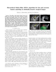
Fig. 1. <strong>MR</strong> <strong>image</strong>s: (a) cardiac; (b) brain; (c) chest and (d) artery.<br />
2009a). However, the FISTA cannot efficiently solve the composite<br />
L1 and TV regularization problem (1), since no efficient algorithm<br />
exists to solve the step<br />
Algorithm 1. FISTA (Beck and Teboulle, 2009b)<br />
Input: q =1/L f , r 1 = x 0 , t 1 =1<br />
<strong>for</strong> k =1to K do<br />
x g = r k qrf(r k )<br />
x k = prox q (g)(x g )<br />
pffiffiffiffiffiffiffiffiffiffiffiffiffiffi<br />
t kþ1 ¼ 1þ 1þ4ðt k Þ 2<br />
2<br />
r kþ1 ¼ x k þ tk 1<br />
ðx k t kþ1 x k 1 Þ<br />
end <strong>for</strong><br />
Algorithm 2. CSD<br />
Input: q ¼ 1=L; a; b; z 0 1 ¼ z0 2 ¼ x g<br />
<strong>for</strong> j =1to J do<br />
x 1 ¼ prox q ð2akxk TV Þðz j 1<br />
1 Þ<br />
x 2 ¼ prox q ð2bkUxk 1 Þðz j 1<br />
2 Þ<br />
x j = (x 1 + x 2 )/2<br />
z j 1 ¼ zj 1<br />
1<br />
þ x j x 1<br />
z j 2 ¼ zj 1<br />
2<br />
þ x j x 2<br />
end <strong>for</strong><br />
x k ¼ prox q ðakxk TV<br />
þ bkUxk 1<br />
Þðx g Þ:<br />
To solve the problem (1), the key problem is thus to develop an efficient<br />
algorithm to solve problem (4). In the following section, we<br />
will show that a scheme based on composite splitting techniques<br />
can be used to do this.<br />
2.2. CSA and FCSA<br />
From the above introduction, we know that, if we can develop a<br />
fast algorithm to solve problem (4), the <strong>MR</strong> <strong>image</strong> <strong>reconstruction</strong><br />
problem can then be efficiently solved by the FISTA, which obtains<br />
p<br />
an -optimal solution in Oð1=<br />
ffiffiffi Þ iterations. Actually, problem (4)<br />
can be considered as a denoising problem:<br />
<br />
<br />
x k 1<br />
¼ arg min<br />
x 2 kx x gk 2 þ qakxk TV<br />
þ qbkUxk 1<br />
: ð5Þ<br />
We use composite splitting techniques to solve this problem: (1)<br />
splitting variable x into two variables {x i } i=1,2 ; (2) per<strong>for</strong>ming operator<br />
splitting over each of {x i } i=1,2 independently and (3) obtaining<br />
the solution x by linear combination of {x i } i=1,2 . We call it Composite<br />
Splitting Denoising (CSD) method, which is outlined in Algorithm 2.<br />
Its validity is guaranteed by the following theorem:<br />
ð4Þ<br />
Theorem 2.2. Suppose {x j } the sequence generated by the CSD. Then,<br />
x j will converge to prox q (akxk TV + bkUxk 1 )(x g ), which means that we<br />
have x j prox q (akxk TV + bkUxk 1 )(x g ).<br />
Sketch Proof of The Theorem 2.2:<br />
Consider a more general <strong>for</strong>mulation:<br />
min FðxÞ f ðxÞþXm g<br />
p i ðB i xÞ<br />
x2R<br />
i¼1<br />
where f is the loss function and {g i } i=1,...,m are the prior models,<br />
both of which are convex functions; {B i } i=1,...,m are orthogonal<br />
matrices.<br />
Proposition 2.1. (Theorem 3.4 in Combettes and Pesquet, 2008):<br />
Let H be a real Hilbert space, and let g ¼ P m<br />
i¼1 g i in C 0 ðHÞ such that<br />
dom g i \ dom g j – ;. Let r 2Hand {x j } be generated by the Algorithm<br />
3. Then, x j will converge to prox(g)(r).<br />
The detailed proof <strong>for</strong> this proposition can be found in Combettes<br />
and Pesquet (2008) and Combettes (2009).<br />
Algorithm 3. (Algorithm 3.1 in Combettes and Pesquet, 2008)<br />
Input: q,{z i } i=1,...,m = r, {w i } i=1,... ,m =1/m,<br />
<strong>for</strong> j =1to J do<br />
<strong>for</strong> i =1to m do<br />
p i,j = prox q (g i /w i )(z j )<br />
end <strong>for</strong><br />
p j ¼ P m<br />
i¼1 w ip i;j<br />
q j+1 = z j + q j x j<br />
k j 2 [0,2]<br />
<strong>for</strong> i =1to m do<br />
z i,j+1 = z i,j+1 + k j (2p j x j p i,j )<br />
end <strong>for</strong><br />
x j+1 = x j + k j (p j x j )<br />
end <strong>for</strong><br />
Suppose that y i ¼ B i x; s i ¼ B T i r and h i(y i )=mqg i (B i x). Because the<br />
operators {B i } i=1,...,m are orthogonal, we can easily obtain that<br />
1<br />
2q kx rk2 ¼ P m<br />
i¼1 2mq 1 ky i s i k 2 . The above problem is transferred<br />
to:<br />
X m <br />
<br />
1<br />
^y i ¼ arg min<br />
yi 2 ky i s i k 2 þ h i ðy i Þ ; x ¼ B T i y i; i ¼ 1; ...; m<br />
i¼1<br />
ð7Þ<br />
Obviously, this problem can be solved by Algorithm 3. According to<br />
Proposition 2.1, we know that x will converge to prox(g)(r). Assuming<br />
g 1 (x)=akxk TV , g 2 (x)=bkxk 1 , m =2, w 1 = w 2 = 1/2 and k j =1, we<br />
obtain the proposed CSD algorithm. x will converge to prox(g)(r),<br />
where g = g 1 + g 2 = akxk TV + bkUxk 1 . h<br />
Combining the CSD with FISTA, a new algorithm FCSA is proposed<br />
<strong>for</strong> <strong>MR</strong> <strong>image</strong> <strong>reconstruction</strong> problem (1). In practice, we<br />
ð6Þ
J. Huang et al. / Medical Image Analysis 15 (2011) 670–679 673<br />
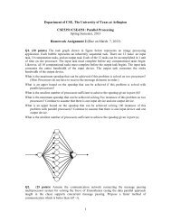
Fig. 2. Cardiac <strong>MR</strong> <strong>image</strong> <strong>reconstruction</strong> from 20% sampling (a) original <strong>image</strong>; (b–f) are the reconstructed <strong>image</strong>s by the CG (Lustig et al., 2007), TVC<strong>MR</strong>I (Ma et al., 2008),<br />
RecPF (Yang et al., 2010), CSA and FCSA. Their SNR are 9.86, 14.43, 15.20, 16.46 and 17.57 (db). Their CPU time are 2.87, 3.14, 3.07, 2.22 and 2.29 (s).<br />
Fig. 3. Brain <strong>MR</strong> <strong>image</strong> <strong>reconstruction</strong> from 20% sampling (a) original <strong>image</strong>; (b–f) are the reconstructed <strong>image</strong>s by the CG (Lustig et al., 2007), TVC<strong>MR</strong>I (Ma et al., 2008),<br />
RecPF (Yang et al., 2010), CSA and FCSA. Their SNR are 8.71, 12.12, 12.40, 18.68 and 20.35 (db). Their CPU time are 2.75, 3.03, 3.00, 2.22 and 2.20 (s).<br />
found that a small iteration number J in the CSD is enough <strong>for</strong> the<br />
FCSA to obtain good <strong>reconstruction</strong> results. Especially, it is set as 1<br />
in our algorithm. Numerous experimental results in the next<br />
section will show that it is good enough <strong>for</strong> real <strong>MR</strong> <strong>image</strong><br />
<strong>reconstruction</strong>.<br />
Algorithm 5 outlines the proposed FCSA. In this algorithm, if we<br />
remove the acceleration step by setting t k+1 1 in each iteration,<br />
we will obtain the Composite Splitting Algorithm (CSA), which is<br />
outlined in Algorithm 4. A key feature of the FCSA is its fast convergence<br />
per<strong>for</strong>mance borrowed from the FISTA. From Theorem 2.1,
674 J. Huang et al. / Medical Image Analysis 15 (2011) 670–679<br />
Fig. 4. Chest <strong>MR</strong> <strong>image</strong> <strong>reconstruction</strong> from 20% sampling (a) original <strong>image</strong>; (b–f) are the reconstructed <strong>image</strong>s by the CG (Lustig et al., 2007), TVC<strong>MR</strong>I (Ma et al., 2008),<br />
RecPF (Yang et al., 2010), CSA and FCSA. Their SNR are 11.80, 15.06, 15.37, 16.53 and 16.07 (db). Their CPU time are 2.95, 3.03, 3.00, 2.29 and 2.234 (s).<br />
Fig. 5. Artery <strong>MR</strong> <strong>image</strong> <strong>reconstruction</strong> from 20% sampling (a) original <strong>image</strong>; (b–f) are the reconstructed <strong>image</strong>s by the CG (Lustig et al., 2007), TVC<strong>MR</strong>I (Ma et al., 2008),<br />
RecPF (Yang et al., 2010), CSA and FCSA. Their SNR are 11.73, 15.49, 16.05, 22.27 and 23.70 (db). Their CPU time are 2.78, 3.06, 3.20, 2.22 and 2.20 (s).<br />
we know that the FISTA can obtain an -optimal solution in<br />
p<br />
Oð1= <br />
ffiffiffi Þ iterations.<br />
Another key feature of the FCSA is that the cost of each iteration<br />
is Oðp logðpÞÞ, as confirmed by the following observations. The step<br />
4, 6 and 7 only involve adding vectors or scalars, thus cost only<br />
OðpÞ or Oð1Þ. In step 1, rf(r k = R T (R r k b)) since f ðr k Þ¼<br />
1<br />
2 kRrk bk 2 in this case. Thus, this step only costs Oðp logðpÞÞ. As<br />
introduced above, the step x k = prox q (2akxk TV )(x g ) can be computed<br />
quickly with cost OðpÞ (Beck and Teboulle, 2009a); The step<br />
x k = prox q (2bkUxk 1 )(x g ) has a close <strong>for</strong>m solution and can be
J. Huang et al. / Medical Image Analysis 15 (2011) 670–679 675<br />
SNR<br />
SNR<br />
20<br />
18<br />
16<br />
14<br />
12<br />
10<br />
8<br />
CG<br />
TVC<strong>MR</strong>I<br />
RecPF<br />
CSA<br />
FCSA<br />
6<br />
0 0.5 1 1.5 2 2.5 3 3.5<br />
CPU Time (s)<br />
18<br />
16<br />
14<br />
12<br />
10<br />
8<br />
(a)<br />
CG<br />
TVC<strong>MR</strong>I<br />
RecPF<br />
CSA<br />
FCSA<br />
6<br />
0 0.5 1 1.5 2 2.5 3 3.5<br />
CPU Time (s)<br />
(c)<br />
SNR<br />
SNR<br />
16<br />
14<br />
12<br />
10<br />
CG<br />
8<br />
TVC<strong>MR</strong>I<br />
RecPF<br />
6<br />
CSA<br />
FCSA<br />
4<br />
0 0.5 1 1.5 2 2.5 3 3.5<br />
CPU Time (s)<br />
(b)<br />
24<br />
22<br />
20<br />
18<br />
16<br />
14<br />
12<br />
CG<br />
TVC<strong>MR</strong>I<br />
10<br />
RecPF<br />
8<br />
CSA<br />
FCSA<br />
6<br />
0 0.5 1 1.5 2 2.5 3 3.5<br />
CPU Time (s)<br />
(d)<br />
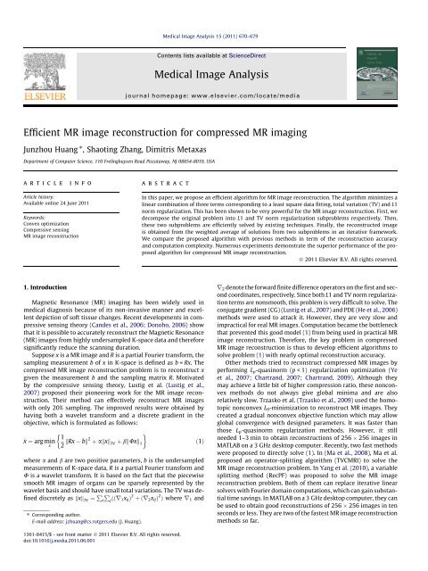
Fig. 6. Per<strong>for</strong>mance comparisons (CPU-Time vs. SNR) on different <strong>MR</strong> <strong>image</strong>s: (a) cardiac <strong>image</strong>; (b) brain <strong>image</strong>; (c) chest <strong>image</strong> and (d) artery <strong>image</strong>.<br />
Table 1<br />
Comparisons of the SNR (db) over 100 runs.<br />
CG TVC<strong>MR</strong>I RecPF CSA FCSA<br />
Cardiac 12.43 ± 1.53 17.54 ± 0.94 17.79 ± 2.33 18.41 ± 0.73 19.26 ± 0.78<br />
Brain 10.33 ± 1.63 14.11 ± 0.34 14.39 ± 2.17 15.25 ± 0.23 15.86 ± 0.22<br />
Chest 12.83 ± 2.05 16.97 ± 0.32 17.03 ± 2.36 17.10 ± 0.31 17.58 ± 0.32<br />
Artery 13.74 ± 2.28 18.39 ± 0.47 19.30 ± 2.55 22.03 ± 0.18 23.50 ± 0.20<br />
Table 2<br />
Comparisons of the CPU Time (s) over 100 runs.<br />
CG TVC<strong>MR</strong>I RecPF CSA FCSA<br />
Cardiac 2.82 ± 0.16 3.16 ± 0.10 2.97 ± 0.12 2.27 ± 0.08 2.30 ± 0.08<br />
Brain 2.81 ± 0.15 3.12 ± 0.15 2.95 ± 0.10 2.27 ± 0.12 2.31 ± 0.13<br />
Chest 2.79 ± 0.16 3.00 ± 0.11 2.89 ± 0.07 2.21 ± 0.06 2.26 ± 0.07<br />
Artery 2.81 ± 0.17 3.04 ± 0.13 2.94 ± 0.09 2.22 ± 0.07 2.27 ± 0.13<br />
computed with cost Oðp logðpÞÞ. In the step x k = project(x k ,[l,u]), the<br />
function x = project(x,[l,u]) is defined as: (1) x = x if l 6 x 6 u; (2)<br />
x = l if x < u; and (3) x = u if x > u, where [l,u] is the range of x. For<br />
example, in the case of <strong>MR</strong> <strong>image</strong> <strong>reconstruction</strong>, we can let l =0<br />
and u = 255 <strong>for</strong> 8-bit gray <strong>MR</strong> <strong>image</strong>s. This step costs OðpÞ. Thus,<br />
the total cost of each iteration in the FCSA is Oðp logðpÞÞ.<br />
With these two key features, the FCSA efficiently solves the <strong>MR</strong><br />
<strong>image</strong> <strong>reconstruction</strong> problem (1) and obtains better <strong>reconstruction</strong><br />
results in terms of both the <strong>reconstruction</strong> accuracy and computation<br />
complexity. The experimental results in the next section<br />
demonstrate its superior per<strong>for</strong>mance compared with all previous<br />
methods <strong>for</strong> <strong>compressed</strong> <strong>MR</strong> <strong>image</strong> <strong>reconstruction</strong>.<br />
Algorithm 4. CSA<br />
Input: q =1/L, a, b, t 1 =1x 0 = r 1<br />
<strong>for</strong> k =1to K do<br />
x g = r k qrf(r k )<br />
x 1 = prox q (2akxk TV )(x g )<br />
x 2 = prox q (2bkUxk 1 )(x g )<br />
x k = (x 1 + x 2 )/2<br />
x k =project (x k ,[l,u])<br />
r k+1 = x k<br />
end<strong>for</strong><br />
Algorithm 5. FCSA<br />
Input: q =1/L, a, b, t 1 =1x 0 = r 1<br />
<strong>for</strong> k =1to K do<br />
x g = r k qrf(r k )<br />
x 1 = prox q (2akxk TV )(x g )<br />
x 2 = prox q (2bkUxk 1 )(x g )<br />
x k = (x 1 + x 2 )/2;<br />
x k =project (x k ,[l,u])<br />
qffiffiffiffiffiffiffiffiffiffiffiffiffiffiffiffiffiffiffiffiffi<br />
t kþ1 ¼ð1 þ 1 þ 4ðt k Þ 2 Þ=2<br />
r k+1 = x k + ((t k 1)/t k+1 )(x k x k 1 )<br />
end <strong>for</strong>
676 J. Huang et al. / Medical Image Analysis 15 (2011) 670–679<br />
Fig. 7. Full Body <strong>MR</strong> <strong>image</strong> <strong>reconstruction</strong> from 25% sampling (a) original <strong>image</strong>; (b–e) are the reconstructed <strong>image</strong>s by the TVC<strong>MR</strong>I (Ma et al., 2008), RecPF (Yang et al., 2010),<br />
CSA and FCSA. Their SNR are 12.56, 13.06, 18.21 and 19.45 (db). Their CPU time are 12.57, 11.14, 10.20 and 10.64 (s).<br />
3. Experiments<br />
3.1. Experiment setup<br />
Suppose a <strong>MR</strong> <strong>image</strong> x has n pixels, the partial Fourier trans<strong>for</strong>m<br />
R in problem (1) consists of m rows of a n n matrix corresponding<br />
to the full 2D discrete Fourier trans<strong>for</strong>m. The m selected<br />
rows correspond to the acquired b. The sampling ratio is defined<br />
as m/n. The scanning duration is shorter if the sampling ratio is<br />
smaller. In <strong>MR</strong> <strong>imaging</strong>, we have certain freedom to select rows,<br />
which correspond to certain frequencies. In the following experiments,<br />
we select the corresponding frequencies according to the<br />
following manner. In the k-space, we randomly obtain more samples<br />
in low frequencies and less samples in higher frequencies.<br />
This sampling scheme has been widely used <strong>for</strong> <strong>compressed</strong> <strong>MR</strong><br />
<strong>image</strong> <strong>reconstruction</strong> (Lustig et al., 2007; Ma et al., 2008; Yang<br />
et al., 2010). Practically, the sampling scheme and speed in <strong>MR</strong><br />
<strong>imaging</strong> also depend on the physical and physiological limitations<br />
(Lustig et al., 2007).<br />
We implement our CSA and FCSA <strong>for</strong> problem (1) and apply<br />
them on 2D real <strong>MR</strong> <strong>image</strong>s. The code that was used <strong>for</strong> the<br />
experiment is available <strong>for</strong> download at the link listed in footnote.<br />
1 All experiments are conducted on a 2.4 GHz PC in Matlab<br />
environment. We compare the CSA and FCSA with the classic <strong>MR</strong><br />
<strong>image</strong> <strong>reconstruction</strong> method based on the CG (Lustig et al.,<br />
2007). We also compare them with two of the fastest <strong>MR</strong> <strong>image</strong><br />
<strong>reconstruction</strong> methods, TVC<strong>MR</strong>I 2 (Ma et al., 2008) and RecPF 3<br />
(Yang et al., 2010). For fair comparisons, we download the codes<br />
from their websites and carefully follow their experiment setup.<br />
For example, the observation measurement b is synthesized as<br />
b = Rx + n, where n is the Gaussian white noise with standard<br />
deviation r = 0.01. The regularization parameter a and b are set<br />
as 0.001 and 0.035. R and b are given as inputs, and x is the unknown<br />
target. For quantitative evaluation, the Signal-to-Noise Ratio<br />
(SNR) is computed <strong>for</strong> each <strong>reconstruction</strong> result. Let x 0 be the<br />
original <strong>image</strong> and x a reconstructed <strong>image</strong>, the SNR is computed<br />
as: SNR = 10 log 10 (V s /V n ), where V n is the Mean Square Error between<br />
the original <strong>image</strong> x 0 and the reconstructed <strong>image</strong> x;<br />
V s = var(x 0 ) denotes the power level of the original <strong>image</strong> where<br />
var(x 0 ) denotes the variance of the values in x 0 .<br />
3.2. Visual comparisons<br />
We apply all methods on four 2D <strong>MR</strong> <strong>image</strong>s: cardiac, brain,<br />
chest and artery respectively. Fig. 1 shows these <strong>image</strong>s. For convenience,<br />
they have the same size of 256 256. The sample ratio is<br />
set to be approximately 20%. To per<strong>for</strong>m fair comparisons, all<br />
methods run 50 iterations except that the CG runs only eight iterations<br />
due to its higher computational complexity.<br />
Figs. 2–5 show the visual comparisons of the reconstructed results<br />
by different methods. The FCSA always obtains the best visual<br />
1 http://paul.rutgers.edu/jzhuang/R_FCSA<strong>MR</strong>I.htm.<br />
2 http://www.columbia.edu/sm2756/TVC<strong>MR</strong>I.htm.<br />
3 http://www.caam.rice.edu/optimization/L1/RecPF/.
J. Huang et al. / Medical Image Analysis 15 (2011) 670–679 677<br />
SNR<br />
SNR<br />
SNR<br />
24<br />
22<br />
20<br />
18<br />
16<br />
14<br />
12<br />
TVC<strong>MR</strong>I<br />
10<br />
RecPF<br />
CSA<br />
8<br />
FCSA<br />
6<br />
0 10 20 30 40 50<br />
Iterations<br />
20<br />
18<br />
16<br />
14<br />
12<br />
10<br />
TVC<strong>MR</strong>I<br />
RecPF<br />
8<br />
CSA<br />
FCSA<br />
6<br />
0 10 20 30 40 50<br />
Iterations<br />
18<br />
16<br />
14<br />
12<br />
10<br />
8<br />
TVC<strong>MR</strong>I<br />
RecPF<br />
6<br />
CSA<br />
FCSA<br />
4<br />
0 10 20 30 40 50<br />
Iterations<br />
(a)<br />
CPU Time (s)<br />
CPU Time (s)<br />
CPU Time (s)<br />
14<br />
12<br />
10<br />
8<br />
6<br />
4<br />
TVC<strong>MR</strong>I<br />
RecPF<br />
2<br />
CSA<br />
FCSA<br />
0<br />
0 10 20 30 40 50<br />
Iterations<br />
14<br />
12<br />
10<br />
8<br />
6<br />
4<br />
TVC<strong>MR</strong>I<br />
RecPF<br />
2<br />
CSA<br />
FCSA<br />
0<br />
0 10 20 30 40 50<br />
Iterations<br />
14<br />
12<br />
10<br />
8<br />
6<br />
4<br />
TVC<strong>MR</strong>I<br />
RecPF<br />
2<br />
CSA<br />
FCSA<br />
0<br />
0 10 20 30 40 50<br />
Iterations<br />
(b)<br />
Fig. 8. Per<strong>for</strong>mance comparisons on the full body <strong>MR</strong> <strong>image</strong> with different sampling ratios. The sample ratios are: (1) 36%; (2) 25% and (3) 20%. The per<strong>for</strong>mance: (a)<br />
Iterations vs. SNR (db) and (b) iterations vs. CPU time (s).<br />
effects on all <strong>MR</strong> <strong>image</strong>s in less CPU time. The CSA is always inferior<br />
to the FCSA, which shows the effectiveness of acceleration<br />
steps in the FCSA <strong>for</strong> the <strong>MR</strong> <strong>image</strong> <strong>reconstruction</strong>. The classical<br />
CG (Lustig et al., 2007) is far worse than others because of its higher<br />
cost in each iteration, the RecPF is slightly better than the<br />
TVC<strong>MR</strong>I, which is consistent with observations in Ma et al.<br />
(2008) and Yang et al. (2010).<br />
In our experiments, these methods have also been applied on<br />
the test <strong>image</strong>s with the sample ratio set to 100%. We observed<br />
that all methods obtain almost the same <strong>reconstruction</strong> results,<br />
with SNR 64.8, after sufficient iterations. This was to be expected,<br />
since all methods are essentially solving the same <strong>for</strong>mulation<br />
‘‘Model (1)’’.<br />
3.3. CPU time and SNRs<br />
Fig. 6 gives the per<strong>for</strong>mance comparisons between different<br />
methods in terms of the CPU time over the SNR. Tables 1 and 2 tabulate<br />
the SNR and CPU Time by different methods, averaged over<br />
100 runs <strong>for</strong> each experiment, respectively. The FCSA always obtains<br />
the best <strong>reconstruction</strong> results on all <strong>MR</strong> <strong>image</strong>s by achieving<br />
the highest SNR in less CPU time. The CSA is always inferior to the<br />
FCSA, which shows the effectiveness of acceleration steps in the<br />
FCSA <strong>for</strong> the <strong>MR</strong> <strong>image</strong> <strong>reconstruction</strong>. While the classical CG (Lustig<br />
et al., 2007) is far worse than others because of its higher cost in<br />
each iteration, the RecPF is slightly better than the TVC<strong>MR</strong>I, which<br />
is consistent to observations in Ma et al. (2008) and Yang et al.<br />
(2010).<br />
3.4. Sample ratios<br />
To test the efficiency of the proposed method, we further per<strong>for</strong>m<br />
experiments on a full body <strong>MR</strong> <strong>image</strong> with size of<br />
924 208. Each algorithm runs 50 iterations. Since we have shown<br />
that the CG method is far less efficient than other methods, we will<br />
not include it in this experiment. The sample ratio is set to be
678 J. Huang et al. / Medical Image Analysis 15 (2011) 670–679<br />
approximately 25%. To reduce the randomness, we run each experiment<br />
100 times <strong>for</strong> each parameter setting of each method. The<br />
examples of the original and recovered <strong>image</strong>s by different algorithms<br />
are shown in Fig. 7. From there, we can observe that the results<br />
obtained by the FCSA are not only visibly better, but also<br />
superior in terms of both the SNR and CPU time.<br />
To evaluate the <strong>reconstruction</strong> per<strong>for</strong>mance with different<br />
sampling ratio, we use sampling ratio 36%, 25% and 20% to obtain<br />
the measurement b respectively. Different methods are then used<br />
to per<strong>for</strong>m <strong>reconstruction</strong>. To reduce the randomness, we run<br />
each experiments 100 times <strong>for</strong> each parameter setting of each<br />
method. The SNR and CPU time are traced in each iteration <strong>for</strong> each<br />
methods.<br />
Fig. 8 gives the per<strong>for</strong>mance comparisons between different<br />
methods in terms of the CPU time and SNR when the sampling ratios<br />
are 36%, 25% and 20% respectively. The <strong>reconstruction</strong> results<br />
produced by the FCSA are far better than those produced by the<br />
CG, TVC<strong>MR</strong>I and RecPF. The <strong>reconstruction</strong> per<strong>for</strong>mance of the<br />
FCSA is always the best in terms of both the <strong>reconstruction</strong> accuracy<br />
and the computational complexity, which further demonstrates<br />
the effectiveness and efficiency of the FCSA <strong>for</strong> the<br />
<strong>compressed</strong> <strong>MR</strong> <strong>image</strong> construction.<br />
3.5. Discussion<br />
The experimental results reported above validate the effectiveness<br />
and efficiency of the proposed composite splitting algorithms<br />
<strong>for</strong> <strong>compressed</strong> <strong>MR</strong> <strong>image</strong> <strong>reconstruction</strong>. Our main contributions<br />
are:<br />
We propose an efficient algorithm (FCSA) to reconstruct the<br />
<strong>compressed</strong> <strong>MR</strong> <strong>image</strong>s. It minimizes a linear combination<br />
of three terms corresponding to a least square data fitting,<br />
total variation (TV) and L1 norm regularization. The computational<br />
complexity of the FCSA is Oðp logðpÞÞ in each iteration<br />
(p is the pixel number in reconstructed <strong>image</strong>). It also has fast<br />
convergence properties. It has been shown to significantly<br />
outper<strong>for</strong>m the classic CG methods (Lustig et al., 2007) and<br />
two state-of-the-art methods (TVC<strong>MR</strong>I (Ma et al., 2008) and<br />
RecPF (Yang et al., 2010)) in terms of both accuracy and<br />
complexity.<br />
The step size in the FCSA is designed according to the inverse<br />
of the Lipschitz constant L f . Actually, using larger values is<br />
known to be a way of obtaining faster versions of the algorithm<br />
(Wright et al., 2009). Future work will study the<br />
combination of this technique with the CSD or FCSA, which is<br />
expected to further accelerate the optimization <strong>for</strong> this kind of<br />
problems.<br />
In this paper, the proposed methods are developed to efficiently<br />
solve model (1), which has been addressed by Sparse<strong>MR</strong>I,<br />
TVC<strong>MR</strong>I and RecPF. There<strong>for</strong>e, with enough iterations, Sparse-<br />
<strong>MR</strong>I, TVC<strong>MR</strong>I and RecPF will obtain the same solution as that<br />
obtained by our methods. Since all of them solve the same <strong>for</strong>mulation,<br />
they will lead to the same gain in in<strong>for</strong>mation content.<br />
In our future work, we will develop new effective<br />
models <strong>for</strong> <strong>compressed</strong> <strong>MR</strong> <strong>image</strong> <strong>reconstruction</strong>, which can<br />
lead to more in<strong>for</strong>mation gains.<br />
4. Conclusion<br />
We have proposed an efficient algorithm <strong>for</strong> the <strong>compressed</strong><br />
<strong>MR</strong> <strong>image</strong> <strong>reconstruction</strong>. Our work has the following contributions.<br />
First, the proposed FCSA can efficiently solve a composite<br />
regularization problem including both TV term and L1 norm term,<br />
which can be easily extended to other medical <strong>image</strong> applications.<br />
Second, the computational complexity of the FCSA is only<br />
Oðp logðpÞÞ in each iteration where p is the pixel number of the<br />
reconstructed <strong>image</strong>. It also has strong convergence properties.<br />
These properties make the real <strong>compressed</strong> <strong>MR</strong> <strong>image</strong> <strong>reconstruction</strong><br />
much more feasible than be<strong>for</strong>e. Finally, we conduct numerous<br />
experiments to compare different <strong>reconstruction</strong> methods.<br />
Our method is shown to impressively outper<strong>for</strong>m the classical<br />
methods and two of the fastest methods so far in terms of both<br />
accuracy and complexity.<br />
References<br />
Beck, A., Teboulle, M., 2009a. Fast gradient-based algorithms <strong>for</strong> constrained total<br />
variation <strong>image</strong> denoising and deblurring problems. IEEE Transaction on Image<br />
Processing 18, 2419–2434.<br />
Beck, A., Teboulle, M., 2009b. A fast iterative shrinkage-thresholding algorithm <strong>for</strong><br />
linear inverse problems. SIAM Journal on Imaging Sciences 2, 183–202.<br />
Candes, E.J., Romberg, J., Tao, T., 2006. Robust uncertainty principles: exact signal<br />
<strong>reconstruction</strong> from highly incomplete frequency in<strong>for</strong>mation. IEEE<br />
Transactions on In<strong>for</strong>mation Theory 52, 489–509.<br />
Chartrand, R., 2007. Exact <strong>reconstruction</strong> of sparse signals via nonconvex<br />
minimization. IEEE Signal Processing Letters 14, 707–710.<br />
Chartrand, R., 2009. Fast algorithms <strong>for</strong> nonconvex compressive sensing: <strong>MR</strong>I<br />
<strong>reconstruction</strong> from very few data. In: Proceedings of the Sixth IEEE<br />
international conference on Symposium on Biomedical Imaging: From Nano<br />
to Macro. IEEE Press, pp. 262–265.<br />
Combettes, P.L., 2009. Iterative construction of the resolvent of a sum of maximal<br />
monotone operators. Journal of Convex Analysis 16, 727–748.<br />
Combettes, P.L., Pesquet, J.C., 2008. A proximal decomposition method <strong>for</strong> solving<br />
convex variational inverse problems. Inverse Problems 24, 1–27.<br />
Combettes, P.L., Wajs, V.R., 2008. Signal recovery by proximal <strong>for</strong>ward-backward<br />
splitting. SIAM Journal on Multiscale Modeling and Simulation 19, 1107–1130.<br />
Donoho, D., 2006. Compressed sensing. IEEE Transactions on In<strong>for</strong>mation Theory 52,<br />
1289–1306.<br />
Eckstein, J., Svaiter, B.F., 2009. General projective splitting methods <strong>for</strong> sums of<br />
maximal monotone operators. SIAM Journal on Control Optimization 48, 787–<br />
811.<br />
Gabay, D., 1983. Chapter IX applications of the method of multipliers to variational<br />
inequalities. Studies in Mathematics and its Applications 15, 299–331.<br />
Gabay, D., Mercier, B., 1976. A dual algorithm <strong>for</strong> the solution of nonlinear<br />
variational problems via finite-element approximations. Computers and<br />
Mathematics with Applications 2, 17–40.<br />
Glowinski, R., Le Tallec, P., 1989. Augmented Lagrangian and Operator-Splitting<br />
Methods in Nonlinear Mechanics, vol. 9. Society <strong>for</strong> Industrial Mathematics.<br />
Goldfarb, D., Ma, S., 2009. Fast Multiple Splitting Algorithms <strong>for</strong> Convex<br />
Optimization. Technical Report, Department of IEOR, Columbia University,<br />
New York.<br />
He, B.S., Liao, L.Z., Han, D., Yang, H., 2002. A new inexact alternating direction<br />
method <strong>for</strong> monotone variational inequalities. Mathematical Programming 92,<br />
103–118.<br />
He, L., Chang, T.C., Osher, S., Fang, T., Speier, P., 2006. <strong>MR</strong> <strong>image</strong> <strong>reconstruction</strong> by<br />
using the iterative refinement method and nonlinear inverse scale space<br />
methods. Technical Report UCLA CAM 06-35. .<br />
Huang, J., Zhang, S., Metaxas, D., 2010. <strong>Efficient</strong> <strong>MR</strong> <strong>image</strong> <strong>reconstruction</strong> <strong>for</strong><br />
<strong>compressed</strong> <strong>MR</strong> <strong>imaging</strong>. In: Proceedings of the 13th International Conference<br />
on Medical Image Computing and Computer-Assisted Intervention: Part I. LNCS,<br />
vol. 6361. Springer-Verlag, pp. 135–142.<br />
Ji, S., Ye, J., 2009. An accelerated gradient method <strong>for</strong> trace norm minimization. In:<br />
Proceedings of the 26th Annual International Conference on Machine Learning.<br />
ACM, pp. 457–464.<br />
Lustig, M., Donoho, D., Pauly, J., 2007. Sparse <strong>MR</strong>I: the application of <strong>compressed</strong><br />
sensing <strong>for</strong> rapid <strong>MR</strong> <strong>imaging</strong>. Magnetic Resonance in Medicine 58, 1182–1195.<br />
Ma, S., Yin, W., Zhang, Y., Chakraborty, A., 2008. An efficient algorithm <strong>for</strong><br />
<strong>compressed</strong> mr <strong>imaging</strong> using total variation and wavelets. In: IEEE<br />
Conference on Computer Vision and Pattern Recognition, CVPR 2008, pp. 1–8.<br />
Malick, J., Povh, J., Rendl, F., Wiegele, A., 2009. Regularization methods <strong>for</strong><br />
semidefinite programming. SIAM Journal on Optimization 20, 336–356.<br />
Nesterov, Y.E., 1983. A method <strong>for</strong> solving the convex programming<br />
problem with convergence rate o(1/k 2 ). Doklady Akademii Nauk SSSR<br />
269, 543–547.<br />
Nesterov, Y.E., 2007. Gradient methods <strong>for</strong> minimizing composite objective<br />
function. Technical Report. .<br />
Spingarn, J.E., 1983. Partial inverse of a monotone operator. Applied Mathematics<br />
and Optimization 10, 247–265.<br />
Trzasko, J., Manduca, A., Borisch, E., 2009. Highly undersampled magnetic resonance<br />
<strong>image</strong> <strong>reconstruction</strong> via homotopic l0-minimization. IEEE Transactions on<br />
Medical Imaging 28, 106–121.<br />
Tseng, P., 1991. Applications of a splitting algorithm to decomposition in convex<br />
programming and variational inequalities. SIAM Journal on Control and<br />
Optimization 29, 119–138.<br />
Tseng, P., 2000. A modified <strong>for</strong>ward-backward splitting method <strong>for</strong> maximal<br />
monotone mappings. SIAM Journal on Control and Optimization 38, 431–446.
J. Huang et al. / Medical Image Analysis 15 (2011) 670–679 679<br />
Wang, Y., Yang, J., Yin, W., Zhang, Y., 2008. A new alternating minimization<br />
algorithm <strong>for</strong> total variation <strong>image</strong> <strong>reconstruction</strong>. SIAM Journal on Imaging<br />
Sciences 1, 248–272.<br />
Wright, S., Nowak, R., Figueiredo, M., 2009. Sparse <strong>reconstruction</strong> by separable<br />
approximation. IEEE Transactions on Signal Processing 57, 2479–2493.<br />
Yang, J., Zhang, Y., Yin, W., 2010. A fast alternating direction method <strong>for</strong> TVL1-L2<br />
signal <strong>reconstruction</strong> from partial fourier data. IEEE Journal of Selected Topics in<br />
Signal Processing 4, 288–297.<br />
Ye, J., Tak, S., Han, Y., Park, H., 2007. Projection <strong>reconstruction</strong> <strong>MR</strong> <strong>imaging</strong> using<br />
focuss. Magnetic Resonance in Medicine 57, 764–775.