Background subtraction using group sparsity and low-rank constraint
Background subtraction using group sparsity and low-rank constraint
Background subtraction using group sparsity and low-rank constraint

Create successful ePaper yourself
Turn your PDF publications into a flip-book with our unique Google optimized e-Paper software.
<strong>Background</strong> Subtraction Using Low Rank<br />
<strong>and</strong> Group Sparsity Constraints<br />
Xinyi Cui 1 , Junzhou Huang 2 , Shaoting Zhang 1 , <strong>and</strong> Dimitris N. Metaxas 1<br />
1 CS Dept., Rutgers University<br />
Piscataway, NJ 08854, USA<br />
2 CSE Dept., Univ. of Texas at Arlington<br />
Arlington, TX, 76019, USA<br />
{xycui,shaoting,dnm}@cs.rutgers.edu,<br />
jzhuang@uta.edu<br />
Abstract. <strong>Background</strong> <strong>subtraction</strong> has been widely investigated in recent<br />
years. Most previous work has focused on stationary cameras. Recently,<br />
moving cameras have also been studied since videos from mobile<br />
devices have increased significantly. In this paper, we propose a unified<br />
<strong>and</strong> robust framework to effectively h<strong>and</strong>le diverse types of videos,<br />
e.g., videos from stationary or moving cameras. Our model is inspired<br />
by two observations: 1) background motion caused by orthographic cameras<br />
lies in a <strong>low</strong> <strong>rank</strong> subspace, <strong>and</strong> 2) pixels belonging to one trajectory<br />
tend to <strong>group</strong> together. Based on these two observations, we introduce<br />
a new model <strong>using</strong> both <strong>low</strong> <strong>rank</strong> <strong>and</strong> <strong>group</strong> <strong>sparsity</strong> <strong>constraint</strong>s. It is<br />
able to robustly decompose a motion trajectory matrix into foreground<br />
<strong>and</strong> background ones. After obtaining foreground <strong>and</strong> background trajectories,<br />
the information gathered on them is used to build a statistical<br />
model to further label frames at the pixel level. Extensive experiments<br />
demonstrate very competitive performance on both synthetic data <strong>and</strong><br />
real videos.<br />
1 Introduction<br />
<strong>Background</strong> <strong>subtraction</strong> is an important preprocessing step in video surveillance<br />
systems. It aims to find independent moving objects in a scene. Many algorithms<br />
have been proposed for background <strong>subtraction</strong> under stationary. In recent years,<br />
videos from moving cameras have also been studied [1] because the number of<br />
moving cameras (such as smart phones <strong>and</strong> digital videos) has increased significantly.<br />
However, h<strong>and</strong>ling diverse types of videos robustly is still a challenging<br />
problem (see the related work in Sec. 2). In this paper, we propose a unified<br />
framework for background <strong>subtraction</strong>, which can robustly deal with videos from<br />
stationary or moving cameras with various number of righd/non-rigid objects.<br />
The proposed method for background <strong>subtraction</strong> is based on two <strong>sparsity</strong><br />
<strong>constraint</strong>s applied on foreground <strong>and</strong> background levels, i.e., <strong>low</strong> <strong>rank</strong> [2] <strong>and</strong><br />
<strong>group</strong> <strong>sparsity</strong> <strong>constraint</strong>s [3]. It is inspired by recently proposed <strong>sparsity</strong> theories<br />
[4, 5]. There are two “<strong>sparsity</strong>” observations behind our method. First, when<br />
A. Fitzgibbon et al. (Eds.): ECCV 2012, Part I, LNCS 7572, pp. 612–625, 2012.<br />
c○ Springer-Verlag Berlin Heidelberg 2012
<strong>Background</strong> Subtraction Using Low Rank <strong>and</strong> Group Sparsity Constraints 613<br />
the scene in a video does not have any foreground moving objects, video motion<br />
has a <strong>low</strong> <strong>rank</strong> <strong>constraint</strong> for orthographic cameras [6]. Thus the motion of<br />
background points forms a <strong>low</strong> <strong>rank</strong> matrix. Second, foreground moving objects<br />
usually occupy a small portion of the scene. In addition, when a foreground<br />
object is projected to pixels on multiple frames, these pixels are not r<strong>and</strong>omly<br />
distributed. They tend to <strong>group</strong> together as a continuous trajectory. Thus these<br />
foreground trajectories usually satisfy the <strong>group</strong> <strong>sparsity</strong> <strong>constraint</strong>.<br />
These two observations provide important information to differentiate independent<br />
objects from the scene. Based on them, the video background <strong>subtraction</strong><br />
problem is formulated as a matrix decomposition problem. First, the video<br />
motion is represented as a matrix on trajectory level (i.e. each row in the motion<br />
matrix is a trajectory of a point). Then it is decomposed into a background<br />
matrix <strong>and</strong> a foreground matrix, where the background matrix is <strong>low</strong> <strong>rank</strong>,<br />
<strong>and</strong> the foreground matrix is <strong>group</strong> sparse. This <strong>low</strong> <strong>rank</strong> <strong>constraint</strong> is able to<br />
automatically model background from both stationary <strong>and</strong> moving cameras, <strong>and</strong><br />
the <strong>group</strong> <strong>sparsity</strong> <strong>constraint</strong> improves the robustness to noise.<br />
The trajectories recognized by the above model can be further used to label<br />
a frame into foreground <strong>and</strong> background at the pixel level. Motion segments on<br />
a video sequence are generated <strong>using</strong> fairly st<strong>and</strong>ard techniques. Then the color<br />
<strong>and</strong> motion information gathered from the trajectories is employed to classify<br />
the motion segments as foreground or background. Our approach is validated on<br />
various types of data, i.e., synthetic data, real-world video sequences recorded<br />
by stationary cameras or moving cameras <strong>and</strong>/or nonrigid foreground objects.<br />
Extensive experiments also show that our method compares favorably to the<br />
recent state-of-the-art methods.<br />
The main contribution of the proposed approach is a new model <strong>using</strong> <strong>low</strong><br />
<strong>rank</strong> <strong>and</strong> <strong>group</strong> <strong>sparsity</strong> <strong>constraint</strong>s to differentiate foreground <strong>and</strong> background<br />
motions. This approach has three merits: 1) The <strong>low</strong> <strong>rank</strong> <strong>constraint</strong> is able<br />
to h<strong>and</strong>le both static <strong>and</strong> moving cameras; 2)The <strong>group</strong> <strong>sparsity</strong> <strong>constraint</strong><br />
leverages the information of neighboring pixels, which makes the algorithm<br />
robust to r<strong>and</strong>om noise; 3) It is relatively insensitive to parameter settings.<br />
2 Related Work<br />
<strong>Background</strong> Subtraction. A considerable amount of work has studied the<br />
problem of background <strong>subtraction</strong> in videos. Here we review a few related<br />
work, <strong>and</strong> please refer to [7] for comprehensive surveys. The mainstream in<br />
the research area of background <strong>subtraction</strong> focuses on stationary cameras.<br />
The earliest background <strong>subtraction</strong> methods use frame difference to detect<br />
foreground [8]. Many subsequent approaches have been proposed to model the<br />
uncertainty in background appearance, such as, but not limited to, W4 [9], single<br />
gaussian model [10], mixture of gaussian [11], non-parametric kernel density [12]<br />
<strong>and</strong> joint spatial-color model [13]. One important variation in stationary camera<br />
based research is the background dynamism. When the camera is stationary, the<br />
background scene may change over time due to many factors (e.g. illumination
614 X. Cui et al.<br />
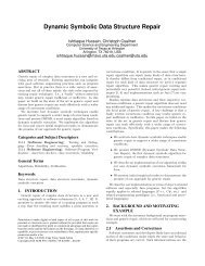
Trajectory level separation<br />
b) Tracked<br />
trajectories<br />
c) Trajectory<br />
matrix<br />
d) Decomposed<br />
trajectories<br />
e) Decomposed trajectories<br />
on original video<br />
a) Input video<br />
h) Output<br />
f) Optical f<strong>low</strong> Pixel level labeling g) Motion segments<br />
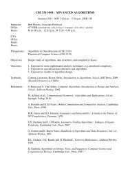
Fig. 1. The framework. Our method takes a raw video sequence as input, <strong>and</strong> produces<br />
a binary labeling as the output. Two major steps are trajectory level separation <strong>and</strong><br />
pixel level labeling.<br />
changes, waves in water bodies, shadows, etc). Several algorithms have been<br />
proposed to h<strong>and</strong>le dynamic background [14–16].<br />
The research for moving cameras has recently attracted people’s attention.<br />
Motion segmentation approaches [17, 18] segment point trajectories based on<br />
subspace analysis. These algorithms provide interesting analysis on sparse trajectories,<br />
though do not output a binary mask as many background <strong>subtraction</strong><br />
methods do. Another popular way to h<strong>and</strong>le camera motion is to have strong<br />
priors of the scene, e.g., approximating background by a 2D plane or assuming<br />
that camera center does not translate [19, 20], assuming a dominant plane [21],<br />
etc. [22] propose a method to use belief propagation <strong>and</strong> Bayesian filtering<br />
to h<strong>and</strong>le moving cameras. Different from their work, long-term trajectories<br />
we use encode more information for background <strong>subtraction</strong>. Recently, [1] has<br />
been proposed to build a background model <strong>using</strong> RANSAC to estimate the<br />
background trajectory basis. This approach assumes that the background motion<br />
spans a three dimensional subspace. Then sets of three trajectories are r<strong>and</strong>omly<br />
selected to construct the background motion space until a consensus set is<br />
discovered, by measuring the projection error on the subspace spanned by the<br />
trajectory set. However, RANSAC based methods are generally sensitive to<br />
parameter selection, which makes it less robust when h<strong>and</strong>ling different videos.<br />
Group <strong>sparsity</strong> [23, 24] <strong>and</strong> <strong>low</strong> <strong>rank</strong> <strong>constraint</strong> [2] have also been applied to<br />
background <strong>subtraction</strong> problem. However, these methods only focus on stationary<br />
camera <strong>and</strong> their <strong>constraint</strong>s are at spatial pixel level. Different from their<br />
work, our method is based on <strong>constraint</strong>s in temporal domain <strong>and</strong> analyzing the<br />
trajectory properties.<br />
3 Methodology<br />
Our background <strong>subtraction</strong> algorithm takes a raw video sequence as input,<br />
<strong>and</strong> generates a binary labeling at the pixel level. Fig. 1 shows our framework.<br />
It has two major steps: trajectory level separation <strong>and</strong> pixel level labeling. In
<strong>Background</strong> Subtraction Using Low Rank <strong>and</strong> Group Sparsity Constraints 615<br />
the first step, a dense set of points is tracked over all frames. We use an offthe-shelf<br />
dense point tracker [25] to produce the trajectories. With the dense<br />
point trajectories, a <strong>low</strong> <strong>rank</strong> <strong>and</strong> <strong>group</strong> <strong>sparsity</strong> based model is proposed to<br />
decompose trajectories into foreground <strong>and</strong> background. In the second step,<br />
motion segments are generated <strong>using</strong> optical f<strong>low</strong> [26] <strong>and</strong> graph cuts [27].<br />
Then the color <strong>and</strong> motion information gathered from the recognized trajectories<br />
builds statistics to label motion segments as foreground or background.<br />
3.1 Low Rank <strong>and</strong> Group Sparsity Based Model<br />
Notations: Given a video sequence, k points are tracked over l frames. Each<br />
trajectory is represented as p i =[x 1i ,y 1i ,x 2i ,y 2i , ...x li ,y li ] ∈ R 1×2l ,wherex <strong>and</strong><br />
y denote the 2D coordinates in each frame. The collection of k trajectories is<br />
represented as a k × 2l matrix, φ =[p T 1 ,p T 2 , ..., p T l ]T , φ ∈ R k×2l .<br />
In a video with moving foreground objects, a subset of k trajectories comes<br />
from the foreground, <strong>and</strong> the rest belongs to the background. Our goal is to<br />
decompose tracked k trajectories into two parts: m background trajectories <strong>and</strong><br />
n foreground trajectories. If we already know exactly which trajectories belong<br />
to the background, then foreground objects can be easily obtained by subtracting<br />
them from k trajectories, <strong>and</strong> vice versa. In other words, φ can be decomposed<br />
as:<br />
φ = B + F, (1)<br />
where B ∈ R k×2l <strong>and</strong> F ∈ R k×2l denote matrices of background <strong>and</strong> foreground<br />
trajectories, respectively. In the ideal case, the decomposed foreground matrix<br />
F consists of n rows of foreground trajectories <strong>and</strong> m rows of flat zeros, while<br />
B has m rows of background trajectories <strong>and</strong> n rows of zeros.<br />
Eq. 1 is a severely under-constrained problem. It is difficult to find B <strong>and</strong> F<br />
without any prior information. In our method, we incorporate two effective priors<br />
to robustly solve this problem, i.e., the <strong>low</strong> <strong>rank</strong> <strong>constraint</strong> for the background<br />
trajectories <strong>and</strong> the <strong>group</strong> <strong>sparsity</strong> <strong>constraint</strong> for the foreground trajectories.<br />
Low Rank Constraint for the <strong>Background</strong>. In a 3D structured scene<br />
without any moving foreground object, video motion solely depends on the scene<br />
<strong>and</strong> the motion of the camera. Our background modeling is inspired from the<br />
fact that B canbefactoredasak × 3 structure matrix of 3D points <strong>and</strong> a 3 × 2l<br />
orthogonal matrix [6]. Thus the background matrix is a <strong>low</strong> <strong>rank</strong> matrix with<br />
<strong>rank</strong> value at most 3. This leads us to build a <strong>low</strong> <strong>rank</strong> <strong>constraint</strong> model for the<br />
background matrix B:<br />
<strong>rank</strong>(B) ≤ 3, (2)<br />
Another <strong>constraint</strong> has been used in the previous research work <strong>using</strong> RANSAC<br />
based method [1]. This work assumes that the background matrix is of <strong>rank</strong><br />
three: <strong>rank</strong>(B) = 3. This is a very strict <strong>constraint</strong> for the problem. We refer<br />
the above two types of <strong>constraint</strong>s as the General Rank model (GR) <strong>and</strong> the<br />
Fixed Rank model (FR). Our GR model is more general <strong>and</strong> h<strong>and</strong>les more<br />
situations. A <strong>rank</strong>-3 matrix models 3D scenes under moving cameras; a <strong>rank</strong>-2
616 X. Cui et al.<br />
matrix models a 2D scene or 3D scene under stationary cameras; a <strong>rank</strong>-1 matrix<br />
is a degenerated case when scene only has one point. The usage of GR model<br />
al<strong>low</strong>s us to develop a unified framework to h<strong>and</strong>le both stationary cameras <strong>and</strong><br />
moving cameras. The experiment section (Sec. 4.2) provides more analysis on<br />
the effectiveness of the GR model when h<strong>and</strong>ling diverse types videos.<br />
Group Sparsity Constraint for the Foreground. Foreground moving objects,<br />
in general, occupy a small portion of the scene. This observation motivates<br />
us to use another important prior, i.e., the number of foreground trajectories<br />
should be smaller than a certain ratio of all trajectories: m ≤ αk, whereα<br />
controls the <strong>sparsity</strong> of foreground trajectories.<br />
Another important observation is that each row in φ represents one trajectory.<br />
Thus the entries in φ are not r<strong>and</strong>omly distributed. They are spatially clustered<br />
within each row. If one entry of the ith row φ i belongs to the foreground,<br />
the whole φ i is also in the foreground. This observation makes the foreground<br />
trajectory matrix F satisfy the <strong>group</strong> <strong>sparsity</strong> <strong>constraint</strong>:<br />
‖F ‖ 2,0 ≤ αk, (3)<br />
where ‖·‖ 2,0 is the mixture of both L 2 <strong>and</strong> L 0 norm. The L 2 norm <strong>constraint</strong> is<br />
applied to each <strong>group</strong> separately (i.e., each row of F ). It ensures that all elements<br />
in the same row are either zero or nonzero at the same time. The L 0 norm<br />
<strong>constraint</strong> is applied to count the nonzero <strong>group</strong>s/rows of F . It guarantees that<br />
only a sparse number of rows are nonzero. Thus this <strong>group</strong> <strong>sparsity</strong> <strong>constraint</strong> not<br />
only ensures that the foreground objects are spatially sparse, but also guarantees<br />
that each trajectory is treated as one unit. Group <strong>sparsity</strong> is a powerful tool in<br />
computer vision problems [28, 23]. The st<strong>and</strong>ard <strong>sparsity</strong> <strong>constraint</strong>, L 0 norm,<br />
(we refer this as Std. sparse method) has been intensively studied in recent<br />
years. However, it does not work well for this problem compared to the <strong>group</strong><br />
<strong>sparsity</strong> one. Std. sparse method treats each element of F independently. It does<br />
not consider any neighborhood information. Thus it is possible that points from<br />
the same trajectory are classified into two classes. In the experiment section<br />
(Sec. 4.1), we discuss the advantage of <strong>group</strong> <strong>sparsity</strong> <strong>constraint</strong> over <strong>sparsity</strong><br />
<strong>constraint</strong> through synthetic data analysis, <strong>and</strong> also show that this <strong>constraint</strong><br />
improves the robustness of our model.<br />
Based on the <strong>low</strong> <strong>rank</strong> <strong>and</strong> <strong>group</strong> <strong>sparsity</strong> <strong>constraint</strong>s, we formulate our<br />
objective function as:<br />
( ) ( ) ˆB, ˆF =argmin ‖ φ − B − F ‖<br />
2<br />
F ,<br />
B,F<br />
s.t. <strong>rank</strong>(B) ≤ 3, ‖ F ‖ 2,0<br />
<strong>Background</strong> Subtraction Using Low Rank <strong>and</strong> Group Sparsity Constraints 617<br />
Trajectory<br />
matrix<br />
Low <strong>rank</strong> matrix<br />
B=UΣV T<br />
Group sparse<br />
matrix F<br />
=<br />
…<br />
…<br />
+<br />
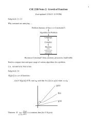
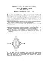
Fig. 2. Illustration of our model. Trajectory matrix φ is decomposed into a background<br />
matrix B <strong>and</strong> a foreground matrix F . B is a <strong>low</strong> <strong>rank</strong> matrix, which only has a<br />
few nonzero eigenvalues (i.e. the diagonal elements of Σ in SVD); F is a <strong>group</strong><br />
sparse matrix. Elements in one row belongs to the same <strong>group</strong> (either foreground or<br />
background), since they lie on one trajectory. The foreground rows are sparse comparing<br />
to all rows. White color denotes zero values, while blue color denotes nonzero values.<br />
datasets. Our method is relatively insensitive to parameter selection. Using α =<br />
0.3 works for all tested videos.<br />
Low <strong>rank</strong> <strong>constraint</strong> is a powerful method in computer vision <strong>and</strong> machine<br />
learning area [29]. Low <strong>rank</strong> <strong>constraint</strong>s <strong>and</strong> Robust PCA have been recently<br />
used to solve vision problems [30, 2, 31], including background <strong>subtraction</strong> at the<br />
pixel level [2]. It assumes that the stationary scenes satisfy a <strong>low</strong> <strong>rank</strong> <strong>constraint</strong>.<br />
However, this assumption does not hold when camera moves. Furthermore, that<br />
formulation does not consider any <strong>group</strong> information, which is an important<br />
<strong>constraint</strong> to make sure neighbor elements are considered together.<br />
3.2 Optimization Framework<br />
This subsection discusses how to effectively solve Eq. 4. The first challenge is that<br />
it is not a convex problem, because of the nonconvexity of the <strong>low</strong> <strong>rank</strong> <strong>constraint</strong><br />
<strong>and</strong> the <strong>group</strong> <strong>sparsity</strong> <strong>constraint</strong>. Furthermore, we also need to simultaneously<br />
recover matrix B <strong>and</strong> F , which is generally a Chicken-<strong>and</strong>-Egg problem.<br />
In our framework, alternating optimization <strong>and</strong> greedy methods are employed<br />
to solve this problem. We first focus on the fixed <strong>rank</strong> problem (i.e., <strong>rank</strong> equals<br />
to 3), <strong>and</strong> then will discuss how to deal with the more general <strong>constraint</strong> of<br />
<strong>rank</strong> ≤ 3.<br />
Eq. 4 is divided into two subproblems with unknown B or F ,<strong>and</strong>solvedby<br />
<strong>using</strong> two steps iteratively:<br />
Step 1: Fix B, <strong>and</strong> update F . The subproblem is:<br />
( ) ( ˆF =argmin ‖ φ ′ − F ‖ 2 )<br />
F , s.t. ‖F ‖2,0
618 X. Cui et al.<br />
To initialize this optimization framework, we simply choose B init = φ, <strong>and</strong><br />
F init = 0. Greedy methods are used to solve both subproblems. To solve Eq. 5,<br />
we compute ‖F i ‖ 2 ,i∈ 1, 2, ..., k, which represents the L 2 norm of each row. Then<br />
the αk rows with largest values are preserved, while the rest rows are set to zero.<br />
This is the estimated F in the first step. In the second step, φ ′′ is computed as per<br />
newly-updated F . To solve Eq. 6. Singular value decomposition (SVD) is applied<br />
on φ ′′ . Then three eigenvectors with largest eigenvalues are used to reconstruct<br />
B. Two steps are alternatively employed until a stable solution of ˆB is found.<br />
Then ˆF is computed as φ − ˆB. The reason of updating ˆF after all iterations is<br />
that the greedy method of solving Eq. 5 discovers exact αk number of foreground<br />
trajectories, which may not be the real foreground number. On the contrary, B<br />
can be always well estimated, since a subset of unknown number of background<br />
trajectories is able to have a good estimation of background subspace. Thus we<br />
finalize ˆF by φ − ˆB. Since the whole framework is based on greedy algorithms,<br />
it does not guarantee a global minimum. In our experiments, however, it is<br />
able to generate reliable <strong>and</strong> stable results. The above-mentioned method solves<br />
the fixed <strong>rank</strong> problem, but the <strong>rank</strong> value in the background problem usually<br />
cannot be pre-determined. To h<strong>and</strong>le this undetermined <strong>rank</strong> issue, we propose<br />
a multiple <strong>rank</strong> iteration method. First, B <strong>and</strong> F are initialized as B (0)<br />
init = φ<br />
<strong>and</strong> F (0)<br />
init = 0k×2l . Then the fixed <strong>rank</strong> optimization procedure is performed on<br />
each specific <strong>rank</strong> starting from 1 to 3. The output of the current fixed <strong>rank</strong><br />
procedure is fed to the next <strong>rank</strong> as its initialization. We obtain the final result<br />
B (3) <strong>and</strong> F (3) in the <strong>rank</strong>-3 iteration. Given a data matrix of K × 2L with K<br />
trajectories over L frames, the major calculation is O(KL 2 ) for SVD on each<br />
iteration. Convergence of each fixed <strong>rank</strong> problem is achieved 6.7 iterations on<br />
average. The overall time complexity is O(KL 2 ).<br />
To explain why our framework works for the general <strong>rank</strong> problem, we discuss<br />
two examples. First, if the <strong>rank</strong> of B is 3 (i.e., moving cameras), then this<br />
framework discovers an optimal solution in the third iteration, i.e., <strong>using</strong> <strong>rank</strong>-3<br />
model. The reason is that the first two iterations, i.e. the <strong>rank</strong>-1 <strong>and</strong> <strong>rank</strong>-<br />
2 models, cannot find the correct solution as they are <strong>using</strong> the wrong <strong>rank</strong><br />
<strong>constraint</strong>s. Second, if the <strong>rank</strong> of the matrix is 2 (i.e., stationary cameras),<br />
then this framework obtains stable solution in the second iteration. This solution<br />
will not be affected in the <strong>rank</strong>-3 iteration. The reason is that the greedy<br />
method is used to solve Eq. 6. When selecting the eigenvectors with three largest<br />
eigenvalues, one of them is simply flat zero. Thus B does not change, <strong>and</strong> the<br />
solution is the same in this iteration. Note that <strong>low</strong> <strong>rank</strong> problems can also<br />
be solved <strong>using</strong> convex relaxation on the <strong>constraint</strong> problem [2]. However, our<br />
greedy method on unconstrained problem is better than convex relaxation in<br />
this application. Convex relaxation is not able to make use of the specific <strong>rank</strong><br />
value <strong>constraint</strong> (≤ 3 in our case). The convex relaxation uses λ to implicitly<br />
constrain the <strong>rank</strong> level, which is hard to constrain a matrix to be <strong>low</strong>er than a<br />
specific <strong>rank</strong> value.
<strong>Background</strong> Subtraction Using Low Rank <strong>and</strong> Group Sparsity Constraints 619<br />
3.3 Pixel Level Labeling<br />
The labeled trajectories from the previous step are then used to label each frame<br />
at the pixel level (i.e. return a binary mask for a frame). In this step, each frame<br />
is treated as an individual labeling task. First, the optical f<strong>low</strong> [26] is calculated<br />
between two consecutive frames. Then motion segments are computed <strong>using</strong><br />
graph cuts [27] on optical f<strong>low</strong>. After collecting the motion segments, we want<br />
to label each motion segment s as f or b, wheref <strong>and</strong> b denotes the label of<br />
foreground <strong>and</strong> background. There are two steps to label the segments. First,<br />
segments with high confidence belonging to f <strong>and</strong> b are selected. Second, a<br />
statistical model is built based on those segments. This model is used to label<br />
segments with <strong>low</strong> confidence. The confidence of a segment is determined by<br />
the number of labeled f <strong>and</strong> b trajectories. The <strong>low</strong> confidence segments are<br />
those ambiguous areas. To predict the labels of these <strong>low</strong> confidence segments,<br />
a statistical model is built for f <strong>and</strong> b based on high confidence ones. First, 20%<br />
pixels are uniformly sampled on segments with high confidence. Each sampled<br />
pixel w is represented by color in hue-saturation space (h, s), optical f<strong>low</strong> (u, v)<br />
<strong>and</strong> position on the frame (x, y). The reason we use sampled points to build<br />
the model instead of the original trajectories is that the sparse trajectories<br />
may not cover enough information (i.e., color <strong>and</strong> positions) on the motion<br />
unit. Uniform sampling covering the whole segment can build a richer model.<br />
The segments are then evaluated <strong>using</strong> a kernel density function:P (s i |c) =<br />
1<br />
N·|s i|<br />
∑ N<br />
i=1<br />
∑<br />
j∈s i<br />
κ(e j − w i ),c ∈ {f,b}, whereκ(·) is the Normal kernel, N<br />
is the total number of sampled pixels, <strong>and</strong> |s i | is the pixel number of s i .For<br />
every pixel j lying on s i , e j denotes the vector containing color, optical f<strong>low</strong> <strong>and</strong><br />
position.<br />
4 Experiments<br />
To evaluate the performance of our algorithm, we conduct experiments on different<br />
data sources: synthetic data, real-world videos from both moving <strong>and</strong><br />
stationary cameras. The performance is evaluated by F -Measure, the harmonic<br />
mean of recall <strong>and</strong> precision. This is a st<strong>and</strong>ard measurement for background<br />
<strong>subtraction</strong> [7, 16]: F =2·recall·precision/(recall+precision). Since our major<br />
contribution is to separate background/foreground motions at trajectory level,<br />
thus our comparisons <strong>and</strong> analysis mainly focus on the first step: trajectory level<br />
labeling.<br />
4.1 Evaluations on Synthetic Data<br />
Experimental Settings. A grid of background points <strong>and</strong> four shapes are<br />
generated to simulate objects moving under camera movements. The homogeneous<br />
representation of each point is (X, Y, Z, 1) as its position in the 3D world.<br />
Then the projected points (x, y) are obtained in a 2D image by (x, y, 1) T =<br />
C · (X, Y, Z, 1) T ,whereC is a 3 × 4 camera projection matrix. The depth value
620 X. Cui et al.<br />
Z in the 3D world for foreground shapes <strong>and</strong> background grid is 10±5<strong>and</strong>20±10,<br />
respectively. The foreground shapes move <strong>and</strong> the background grid stays still.<br />
Changing the camera projection matrix C simulates the camera movement <strong>and</strong><br />
generates projected images.<br />
Group Sparsity Constraint<br />
versus St<strong>and</strong>ard Sparsity<br />
Constraint. We compare the<br />
performance between the <strong>group</strong><br />
<strong>sparsity</strong> <strong>constraint</strong> (L 2,0 norm)<br />
<strong>and</strong> Std. sparse <strong>constraint</strong><br />
(L 0 norm). The <strong>sparsity</strong> <strong>constraint</strong><br />
aims to find a sparse<br />
set of nonzero elements, which<br />
is ‖F ‖ 0 < αk × 2l in our<br />
problem. k × 2l denotes the<br />
total number of nonzero elements.<br />
It is equivalent to the<br />
total number of nonzero elements<br />
in the <strong>group</strong> <strong>sparsity</strong><br />
F-Measure<br />
(a) Stationary Camera<br />
1<br />
0.8<br />
0.6<br />
0.4<br />
0.2<br />
0<br />
0 50 100<br />
Variance<br />
F-Measure<br />
1<br />
0.8<br />
0.6<br />
0.4<br />
0.2<br />
(b) Moving Camera<br />
L20<br />
L0<br />
0<br />
0 20 40<br />
Variance<br />
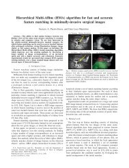
Fig. 3. Comparison between <strong>group</strong> <strong>sparsity</strong> <strong>constraint</strong><br />
(L 2,0 norm) <strong>and</strong> Std. sparse <strong>constraint</strong>. The<br />
left is synthetic data simulated with a stationary<br />
camera, <strong>and</strong> the right is simulated with a moving<br />
camera.<br />
<strong>constraint</strong>. Note that the formulation with this Std. sparse method is similar<br />
to Robust PCA method [2]. The difference is that we use it at the trajectory<br />
level instead of pixel level.<br />
Two sets of data are generated to evaluate the performance. One is simulated<br />
with a stationary camera, <strong>and</strong> the other is from a moving one. Foreground keeps<br />
moving in the whole video sequence. R<strong>and</strong>om noise with variance v is added to<br />
both the foreground moving trajectories <strong>and</strong> camera projection matrix C. The<br />
performance is shown in Fig. 3. In the noiseless case (i.e. v = 0), the motion<br />
pattern from the foreground is distinct from the background in the whole video<br />
sequence. Thus each element on the foreground trajectories is different from<br />
the background element. Sparsity <strong>constraint</strong> produces the same perfect result as<br />
<strong>group</strong> <strong>sparsity</strong> <strong>constraint</strong>. When v goes up, the distinction of elements between<br />
foreground <strong>and</strong> background goes down. Thus some elements from the foreground<br />
may be recognized as background. On the contrary, the <strong>group</strong> <strong>sparsity</strong> <strong>constraint</strong><br />
connects the elements in the neighboring frames. It treats the elements on one<br />
trajectory as one unit. Even some elements on this trajectories are similar to<br />
the background, the distinction along the whole trajectory is still large from the<br />
background. As shown in Fig. 3, <strong>using</strong> the <strong>group</strong> <strong>sparsity</strong> <strong>constraint</strong> is more<br />
robust than <strong>using</strong> the <strong>sparsity</strong> <strong>constraint</strong> when variance increases.<br />
4.2 Evaluations on Videos<br />
Experimental Settings. We test our algorithm on publicly available videos<br />
from various sourcese. One video source is provided by S<strong>and</strong> <strong>and</strong> Teller [32]<br />
(refer this as ST sequences). ST sequences are recorded with h<strong>and</strong> held cameras,<br />
both indoors <strong>and</strong> outdoors, containing a variety of non-rigidly deforming objects
<strong>Background</strong> Subtraction Using Low Rank <strong>and</strong> Group Sparsity Constraints 621<br />
(h<strong>and</strong>s, faces <strong>and</strong> bodies). They are high resolution images with large frame-toframe<br />
motion <strong>and</strong> significant parallax. Another source of videos is provided from<br />
Hopkins 155 dataset [33], witch has two or three motions from indoor <strong>and</strong> outdoor<br />
scenes. These sequences contain degenerate <strong>and</strong> non-degenerate motions,<br />
independent <strong>and</strong> partially dependent motions, articulated <strong>and</strong> non-rigid motions.<br />
We also test our algorithm on a typical video for stationary camera: “truck”.<br />
The trajectories in these sequences were created <strong>using</strong> an off-the-shelf dense<br />
particle tracker [25]. We manually label the pixels into foreground/background<br />
(binary maps). If a trajectory falls into the foreground area, it is considered as<br />
foreground, <strong>and</strong> verse versa.<br />
H<strong>and</strong>ling Stationary <strong>and</strong> Moving<br />
Cameras. We first demonstrate<br />
that our approach h<strong>and</strong>les<br />
both stationary cameras <strong>and</strong><br />
moving cameras automatically in<br />
a unified framework, by <strong>using</strong> the<br />
General Rank <strong>constraint</strong> (GR) instead<br />
of the Fixed Rank <strong>constraint</strong><br />
(FR). We use two videos<br />
to show the difference. One is<br />
“VH<strong>and</strong>” from a moving camera<br />
(<strong>rank</strong>(B) = 3), <strong>and</strong> the other<br />
is “truck” captured by stationary<br />
camera (<strong>rank</strong>(B) = 2). We use<br />
3000<br />
2000<br />
1000<br />
3000<br />
2000<br />
1000<br />
GR Rank 1<br />
0<br />
0 0.5 1<br />
0<br />
0 0.5 1<br />
150<br />
100<br />
50<br />
GR Rank 2<br />
0<br />
0 0.5 1<br />
150<br />
100<br />
50<br />
0<br />
0 0.5 1<br />
60<br />
40<br />
20<br />
GR Rank 3<br />
0<br />
0 0.5 1<br />
150<br />
100<br />
50<br />
0<br />
0 0.5 1<br />
60<br />
40<br />
20<br />
FR Rank 3<br />
0<br />
0 0.5 1<br />
30<br />
20<br />
10<br />
0<br />
0 0.5 1<br />
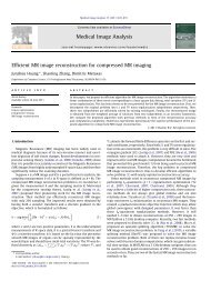
Fig. 4. ‖ ˆF i‖ 2 distribution of the GR <strong>and</strong> the FR<br />
model. Green means foreground <strong>and</strong> blue means<br />
background. Separation means good result. Top<br />
row is from moving camera, <strong>and</strong> bottom row is<br />
from stationary camera. The four columns are<br />
GR−1, GR−2, GR−3 <strong>and</strong>FR.<br />
the distribution of L 2 norms of<br />
estimated foreground trajectories<br />
(i.e., ‖ ˆF i ‖ 2 ,i ∈ 1, 2, ..., k) to show how well background <strong>and</strong> foreground is<br />
separated in our model. For a good separation result, F should be well estimated.<br />
Thus ‖ ˆF i ‖ 2 is large for foreground trajectories <strong>and</strong> small for background ones.<br />
In other words, its distribution has an obvious difference between the foreground<br />
region <strong>and</strong> the background region (see examples in Fig. 4).<br />
We use GR-i, i ∈ 1, 2, 3 to denote the optimization iteration on each <strong>rank</strong><br />
value. ‖ ˆF i ‖ 2 of each specific <strong>rank</strong> iteration is plotted in Fig. 4. The GR method<br />
works for both cases. When the <strong>rank</strong> of B is 3 (the first row of Fig. 4), the<br />
FR model also finds a good solution, since <strong>rank</strong>-3 perfectly fits the FR model.<br />
However, the FR <strong>constraint</strong> fails when the <strong>rank</strong> of B is 2, where the distribution<br />
of ‖ ˆF i ‖ 2 between B <strong>and</strong> F are mixed together. On the other h<strong>and</strong>, GR−2 can<br />
h<strong>and</strong>le this well, since the data perfectly fits the <strong>constraint</strong>. On GR−3 stage, it<br />
uses the result from GR−2 as the initialization, thus the result on GR−3 still<br />
holds. The figure shows that the distribution of ‖ ˆF i ‖ 2 from the two parts has<br />
been clearly separated in the third column of the bottom row. This experiment<br />
demonstrates that the GR model can h<strong>and</strong>le more situations than the FR model.<br />
Since in real applications it is hard to know the specific <strong>rank</strong> value in advance,<br />
the GR model provides a more flexible way to find the right solution.
622 X. Cui et al.<br />
Table 1. Quantitative evaluation at trajectory level labeling<br />
RANS GPCA LSA RANS Std. Ours<br />
AC-b<br />
AC-m Sparse<br />
VPerson 0.786 0.648 0.912 0.656 0.616 0.981<br />
VH<strong>and</strong> 0.952 0.932 0.909 0.930 0.132 0.987<br />
VCars 0.867 0.316 0.145 0.276 0.706 0.993<br />
cars2 0.750 0.773 0.568 0.958 0.625 0.976<br />
cars5 0.985 0.376 0.054 0.637 0.779 0.990<br />
people1 0.932 0.564 0.087 0.743 0.662 0.955<br />
truck 0.351 0.368 0.140 0.363 0.794 0.975<br />
Input<br />
video<br />
RANSAC-b GPCA LSA RANSAC-m St<strong>and</strong>ard sparse Our method<br />
Fig. 5. Results at trajectory level labeling. Green: foreground; purple: background.<br />
From top to bottom, five videos are “VCars”, “cars2 ”, “cars5 ”, “people1 ” <strong>and</strong><br />
“VH<strong>and</strong>”.<br />
Performance Evaluation on Trajectory Labeling. We compare our method<br />
with four state-of-art algorithms: RANSAC-based background <strong>subtraction</strong> (referred<br />
as RANSAC-b here) [1], Generalized GPCA (GPCA) [34], Local Subspace<br />
Affinity (LSA) [18] <strong>and</strong> motion segmentation <strong>using</strong> RANSAC (RANSAC-m)<br />
[33]. GPCA, LSA <strong>and</strong> RANSAC-m are motion segmentation algorithms <strong>using</strong><br />
subspace analysis for trajectories. The code of these algorithms are available<br />
online. When testing these methods, we use the same trajectories as for our own<br />
method. Since LSA method runs very s<strong>low</strong> when <strong>using</strong> trajectories more than<br />
5000, we r<strong>and</strong>omly sample 5000 trajectories for each test video. The three motion
<strong>Background</strong> Subtraction Using Low Rank <strong>and</strong> Group Sparsity Constraints 623<br />
segmentation algorithms ask for the number of regions to be given in advance.<br />
We provide the correct number of segments n, whereas our method does not need<br />
that. Motion segmentation methods separate trajectories into n segments. Here<br />
we treat the segment with the largest trajectory number as the background <strong>and</strong><br />
rest as the foreground. For RANSAC-b method, two major parameters influence<br />
the performance: projection error threshold th <strong>and</strong> consensus percentage p.<br />
Inappropriate selection of parameters may result in failure of finding the correct<br />
result.Inaddition,asRANSAC-b r<strong>and</strong>omly selects three trajectories in each<br />
round, it may end up with finding a subspace spanned by part of foreground<br />
<strong>and</strong> background. The result it generates is not stable. Running the algorithm<br />
multiple times may give different separation of background <strong>and</strong> foreground,<br />
which is undesirable. In order to have a fair comparison with it, we grid search<br />
the best parameter set over all teste videos <strong>and</strong> report the performance under<br />
the optimal parameters.<br />
The quantitative <strong>and</strong> qualitative results on the trajectory level separation<br />
is shown in Fig. 5 <strong>and</strong> Tab. 1, respectively. Our method works well for the test<br />
videos. Take “cars5 ” for example. GPCA <strong>and</strong> LSA misclassify some trajectories.<br />
RANSAC-b r<strong>and</strong>omly selects three trajectories to build the scene motion. On this<br />
frame, the three r<strong>and</strong>om trajectories all lie in the middle region. The background<br />
model built from these 3 trajectories do not cover the left <strong>and</strong> right region of the<br />
scene, thus the left <strong>and</strong> right regions are misclassified as foreground. RANSAC-m<br />
produces similar behavior to RANSAC-b. Std. sparse method does not have any<br />
<strong>group</strong> <strong>constraint</strong> in the consecutive frames, thus some trajectories are classified<br />
as foreground in one frame, <strong>and</strong> classified as background in the next frame. Note<br />
that the quantitative results are obtained by averaging on all frames over 50<br />
iterations. Fig. 5 only shows performance on one frame, which may not reflect<br />
the overall performance shown in Tab. 1.<br />
Performance Evaluation at Pixel Level Labeling. We also evaluate the performance<br />
at the pixel level <strong>using</strong> four methods: RANSAC-b [1], MoG [11], Std.<br />
sparse method <strong>and</strong> the proposed method. GPCA, LSA, RANSAC-m are not evaluated<br />
in this part, since these three algorithms do not provide pixel level labeling.<br />
Due to space limitations, one typical video “VPerson” is shown here in Fig. 6.<br />
MoG does not perform well, because a statistical model of MoG is built on<br />
pixels of fixed positions over multiple frames, but background objects do not stay<br />
in the fixed positions under moving cameras. RANSAC-b can accurately label<br />
Fig. 6. Quantitative results at pixel level labeling on “VPerson” sequence
624 X. Cui et al.<br />
pixels if the trajectories are well classified. However, it is also possible to build<br />
a wrong background subspace because RANSAC-b is not stable <strong>and</strong> sensitive to<br />
parameter selection. Our method can robustly h<strong>and</strong>le these diverse types of data,<br />
due to our generalized <strong>low</strong> <strong>rank</strong> <strong>constraint</strong> <strong>and</strong> <strong>group</strong> <strong>sparsity</strong> <strong>constraint</strong>. One<br />
limitation of our method is that it classifies the shadow as part of the foreground<br />
(e.g., on the left side of the person in “VPerson” video). This could be further<br />
refined by <strong>using</strong> shadow detection/removal techniques [16].<br />
5 Conclusions <strong>and</strong> Future Work<br />
In this paper, we propose an effective approach to do background <strong>subtraction</strong><br />
for complex videos by decomposing the motion trajectory matrix into a <strong>low</strong> <strong>rank</strong><br />
one <strong>and</strong> a <strong>group</strong> <strong>sparsity</strong> one. Then the information from these trajectories is<br />
used to further label foreground at the pixel level. Extensive experiments are<br />
conducted on both synthetic data <strong>and</strong> real videos to show the benefits of our<br />
model. The <strong>low</strong> <strong>rank</strong> <strong>and</strong> <strong>group</strong> <strong>sparsity</strong> <strong>constraint</strong>s make the model robust to<br />
noise <strong>and</strong> h<strong>and</strong>le diverse types of videos.<br />
Our method depends on trajectory-tracking technique, which is also an active<br />
research area in computer vision. When the tracking technique fails, our<br />
method may not work well. A robust way is to build the tracking errors into the<br />
optimization formulation. We will investigate it in our future work.<br />
References<br />
1. Sheikh, Y., Javed, O., Kanade, T.: <strong>Background</strong> <strong>subtraction</strong> for freely moving<br />
cameras. In: ICCV (2009)<br />
2. C<strong>and</strong>es, E.J., Li, X., Ma, Y., Wright, J.: Robust principal component analysis<br />
Journal of ACM (2011)<br />
3. Yuan, M., Lin, Y.: Model selection <strong>and</strong> estimation in regression with <strong>group</strong>ed<br />
variables. Journals of the Royal Statistical Society (2006)<br />
4. C<strong>and</strong>es, E., Tao, T.: Near-optimal signal recovery from r<strong>and</strong>om projections:<br />
Universal encoding strategies TIT (2006)<br />
5. Starck, J.L., Elad, M., Donoho, D.: Image decomposition via the combination of<br />
sparse representations <strong>and</strong> a variational approach. TIP (2005)<br />
6. Tomasi, C., Kanade, T.: Shape <strong>and</strong> motion from image streams under orthography:<br />
a factorization method. IJCV (1992)<br />
7. Brutzer, S., Hoferlin, B., Heidemann, G.: Evaluation of background <strong>subtraction</strong><br />
techniques for video surveillance. In: CVPR (2011)<br />
8. Jain, R., Nagel, H.: On the analysis of accumulative difference pictures from image<br />
sequences of real world scenes. TPAMI (2009)<br />
9. Haritaoglu, I., Harwood, D., Davis, L.: W4: real-time surveillance of people <strong>and</strong><br />
their activities. TPAMI (2000)<br />
10. Wren, C., Azarbayejani, A., Darrell, T., Pentl<strong>and</strong>, A.: Pfinder: Real-time tracking<br />
of the human body. TPAMI (2002)<br />
11. Stauffer, C., Grimson, W.: Learning patterns of activity <strong>using</strong> real-time tracking.<br />
TPAMI (2000)<br />
12. Elgammal, A., Duraiswami, R., Harwood, D., Davis, L.: <strong>Background</strong> <strong>and</strong> foreground<br />
modeling <strong>using</strong> nonparametric kernel density estimation for visual surveillance.<br />
Proceedings of the IEEE (2002)
<strong>Background</strong> Subtraction Using Low Rank <strong>and</strong> Group Sparsity Constraints 625<br />
13. Sheikh, Y., Shah, M.: Bayesian object detection in dynamic scenes. In: CVPR<br />
(2005)<br />
14. Monnet, A., Mittal, A., Paragios, N., Ramesh, V.: <strong>Background</strong> modeling <strong>and</strong><br />
<strong>subtraction</strong> of dynamic scenes. In: ICCV (2003)<br />
15. Zhong, J., Sclaroff, S.: Segmenting foreground objects from a dynamic textured<br />
background via a robust kalman filter. In: ICCV (2003)<br />
16. Liao, V.S., Zhao, G., Kellokumpu, Pietikainen, M., Li, S.Z.: Modeling pixel process<br />
with scale invariant local patterns for background <strong>subtraction</strong> in complex scenes.<br />
In: CVPR (2010)<br />
17. Rao, S., Tron, R., Vidal, R., Ma, Y.: Motion segmentation in the presence of<br />
outlying, incomplete, or corrupted trajectories. TPAMI (2010)<br />
18. Yan, J., Pollefeys, M.: A General Framework for Motion Segmentation: Independent,<br />
Articulated, Rigid, Non-rigid, Degenerate <strong>and</strong> Non-degenerate. In: Leonardis,<br />
A., Bischof, H., Pinz, A. (eds.) ECCV 2006, Part IV. LNCS, vol. 3954, pp. 94–106.<br />
Springer, Heidelberg (2006)<br />
19. Hayman, E., Eklundh, J.-O.: Statistical background <strong>subtraction</strong> for a mobile<br />
observer. In: ICCV (2003)<br />
20. Ren, Y., Chua, C., Ho, Y.: Statistical background modeling for non-stationary<br />
camera. PR Letters (2003)<br />
21. Yuan, C., Medioni, G., Kang, J., Cohen, I.: Detecting motion regions in the<br />
presence of a strong parallax from a moving camera by multiview geometric<br />
<strong>constraint</strong>s. TPAMI (2007)<br />
22. Kwak, S., Lim, T., Nam, W., Han, B., Han, J.H.: Generalized background<br />
<strong>subtraction</strong> based on hybrid inference by belief propagation <strong>and</strong> bayesian filtering.<br />
In: ICCV (2011)<br />
23. Huang, J., Zhang, T.: The benefit of <strong>group</strong> <strong>sparsity</strong>. The Annals of Statistics (2010)<br />
24. Huang, J., Huang, X., Metaxas, D.: Learning with dynamic <strong>group</strong> <strong>sparsity</strong>. In:<br />
ICCV, pp. 64–71 (2009)<br />
25. Sundaram, N., Brox, T., Keutzer, K.: Dense Point Trajectories by GPU-<br />
Accelerated Large Displacement Optical F<strong>low</strong>. In: Daniilidis, K., Maragos, P.,<br />
Paragios, N. (eds.) ECCV 2010, Part I. LNCS, vol. 6311, pp. 438–451. Springer,<br />
Heidelberg (2010)<br />
26. Liu, C.: Beyond pixels: Exploring new representations <strong>and</strong> applications for motion<br />
analysis. Doctoral thesis, Massachusetts Institute of Technology (2009)<br />
27. Boykov, Y., Veksler, O., Zabih, R.: Fast approximate energy minimization via<br />
graph cuts. TPAMI (2001)<br />
28. Zhang, S., Huang, J., Huang, Y., Yu, Y., Li, H., Metaxas, D.: Automatic image<br />
annotation <strong>using</strong> <strong>group</strong> <strong>sparsity</strong>. In: CVPR (2010)<br />
29. Liu, G., Lin, Z., Yu, Y.: Robust subspace segmentation by <strong>low</strong>-<strong>rank</strong> representation.<br />
In: ICML (2010)<br />
30. Zhang, Z., Liang, X., Ma, Y.: Unwrapping <strong>low</strong>-<strong>rank</strong> textures on generalized<br />
cylindrical surfaces. In: ICCV (2011)<br />
31. Mu, Y., Dong, J., Yuan, X., Yan, S.: Accelerated <strong>low</strong>-<strong>rank</strong> visual recovery by<br />
r<strong>and</strong>om projection. In: CVPR (2011)<br />
32. S<strong>and</strong>, P., Teller, S.: Particle video: Long-range motion estimation <strong>using</strong> point<br />
trajectories. In: CVPR (2006)<br />
33. Tron, R., Vidal, R.: A benchmark for the comparison of 3-D motion segmentation<br />
algorithms. In: CVPR (2007)<br />
34. R., Vidal, Y.M., Sastry, S.: Generalized principal component analysis (GPCA). In:<br />
CVPR (2003)