Assignment 7: Simulink and Modeling Systems Problem 1
Assignment 7: Simulink and Modeling Systems Problem 1
Assignment 7: Simulink and Modeling Systems Problem 1

Create successful ePaper yourself
Turn your PDF publications into a flip-book with our unique Google optimized e-Paper software.
CEE 3804: Computer Applications in Civil Engineering Spring 2011<br />
<strong>Assignment</strong> 7: <strong>Simulink</strong> <strong>and</strong> <strong>Modeling</strong> <strong>Systems</strong><br />
Solution<br />
<strong>Problem</strong> 1<br />
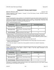
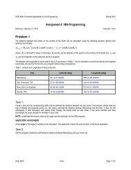
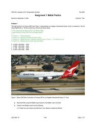
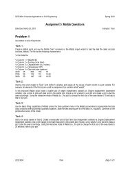
Your task is design an emergency exit ramp for a runaway truck. Figure 1 illustrates the situation.<br />
Instructor: Trani<br />
Figure 1. Emergency Exit Ramp.<br />
The truck has a mass of 40,000 kg. <strong>and</strong> enters the ramp at a speed of 42 m/s (~80 mph) while on a -5% grade. The ramp is<br />
constructed in two segments: a) curved section with a radius of 1000 meters <strong>and</strong> b) straight section with a grade of 15%.<br />
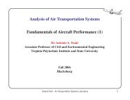
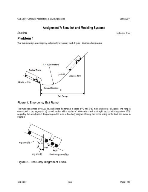
neglecting the aerodynamic drag acting on the truck, a free-body diagram showing the forces acting on the truck are shown in<br />
Figure 2.<br />
Figure 2. Free Body Diagram of Truck.<br />
CEE 3804 Trani Page 1 of 9
Define a common set notation to solve the problem. When the truck is going downhill, the gravity force helps accelerate the<br />
truck. When is going uphill the gravity force helps slow down the motion. The fundamental equation of motion to describe the<br />
deceleration of the truck on the exit ramp is:<br />
m dV<br />
dt<br />
= −mgcos(δ )µ + mgsin(δ )<br />
Here we adopt the nomenclature that when angle δ is positive (i,e., downhill) the term mgsin(δ ) will be positive <strong>and</strong> thus<br />
opposite to the friction term. In this case, the gravity helps accelerate the truck. When going uphill δ is negative <strong>and</strong> the term<br />
mgsin(δ ) is negative helping decelerate the truck.<br />
Task 1<br />
Model the curved section of the road as either a series of line segments or by deriving an equation that relates the local grade of<br />
the curve as a function of the path length along the curve.<br />
The curved section is made of two segments: a) a downhill segment ( l 1<br />
) <strong>and</strong> an uphill segment ( l 2<br />
). The length of these<br />
segments is easily calculated below:<br />
l 1<br />
= G 1<br />
100<br />
l 2<br />
= G 2<br />
100<br />
⎡ 2π R ⎤<br />
⎢<br />
⎣(2π )<br />
⎥<br />
⎦<br />
= −5 (1000m) = 50 meters<br />
100<br />
⎡ 2π R ⎤<br />
⎢<br />
⎣(2π )<br />
⎥<br />
⎦<br />
= 15 (1000m) = 150 meters<br />
100<br />
The total length of the curved segment is then 150 meters.<br />
For the curved road of radius 1,000 meters the grade decreases at a rate of 1/1000 radians per meter (i.e., 0.05 radians in 50<br />
meters for the first segment of the road). An equation that relates the local grade of the road with path length (s) is then,<br />
⎛<br />
G(s) = G 1<br />
−<br />
dG ⎞<br />
⎝<br />
⎜<br />
ds ⎠<br />
⎟ s<br />
G(s) = 0.05 − ( 0.001)s<br />
where:<br />
⎛<br />
⎝<br />
⎜<br />
dG<br />
ds<br />
⎞<br />
⎠<br />
⎟ is the rate of change of the grade (in radians/meter) vs.path distance traveled (s), G 1<br />
is the initial grade of the<br />
road (in radians) <strong>and</strong> s is the path length along the curved section of the road in meters. verify this equation by examining the<br />
value of G(s) when s = 200 meters ( G(200) = −0.15 radians). This equation can be discretized as a table function by<br />
selecting values of grade vs. path distance. For example, if 10 segments are selected along the path, the values of G(s) are<br />
shown in Table 1 in table lookup function.<br />
Path Length (m)<br />
Grade (Rad.)<br />
0 0.0500000000000000<br />
20 0.0300000000000000<br />
40 0.0100000000000000<br />
60 -0.0100000000000000<br />
CEE 3804 Trani Page 2 of 9
Path Length (m)<br />
Grade (Rad.)<br />
80 -0.0300000000000000<br />
100 -0.0500000000000000<br />
120 -0.0700000000000000<br />
140 -0.0900000000000000<br />
160 -0.110000000000000<br />
180 -0.130000000000000<br />
200 -0.150000000000000<br />
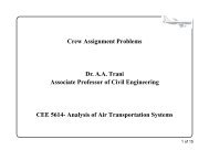
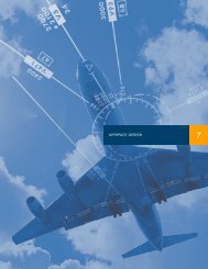
Figure 3. <strong>Simulink</strong> Model to Model Runaway Truck. Equation Used to Relate Grade <strong>and</strong><br />
Path Length (s).<br />
According to this model, 334.4 meters are needed to bring truck to a full stop at<br />
the end of the hill.<br />
CEE 3804 Trani Page 3 of 9
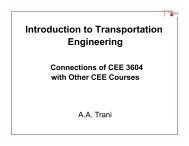
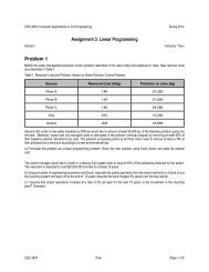
Figure 4. Acceleration, Speed <strong>and</strong> Distance Profiles for Truck. Equation Used to Relate<br />
Grade <strong>and</strong> Path Length (s).<br />
CEE 3804 Trani Page 4 of 9
Figure 5. <strong>Simulink</strong> Model to Model Runaway Truck. Table Lookup Function Used to<br />
Relate Grade <strong>and</strong> Path Length (s).<br />
Figure 6. Lookup Table Values to Relate Grade <strong>and</strong> Path Length. Vector of Input Values<br />
are Path Length. Table Data is the Grade in Radians.<br />
CEE 3804 Trani Page 5 of 9
Figure 7. Acceleration, Speed <strong>and</strong> Distance Profiles for Truck. Table Lookup Function<br />
Used to Relate Grade <strong>and</strong> Path Length (s).<br />
According to this model, 334.5 meters are needed to bring truck to a full stop at<br />
the end of the hill.<br />
CEE 3804 Trani Page 6 of 9
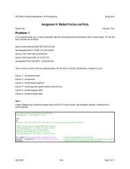
<strong>Problem</strong> 2<br />
An Excel file contains data for thous<strong>and</strong>s of public airports in the U.S. A sample of the file is shown below. The file is called<br />
airports_2011.xls.<br />
Task 1<br />
Create a Matlab script <strong>and</strong> use the Matlab function xlsread to read the data file into a Matalb Cell Array. Rename the variables<br />
with names that represent the data. The airport name is a 3-letter code used by the FAA to name airports (column 1).<br />
___________ Matlab Script ___________<br />
% Script file for Task1 of <strong>Problem</strong> 2 (<strong>Assignment</strong> 7)<br />
% Read the file using the xlsread comm<strong>and</strong> in Matlab<br />
% reads numeric <strong>and</strong> text sections seperately<br />
[num txt]=xlsread('airports_2011.xls');<br />
% Define variables in the problem<br />
header=txt(1,:); % header is the first row of the file read<br />
txt(1,:)=[];<br />
airportID=txt(:,1);<br />
name=txt(:,2);<br />
state=txt(:,3);<br />
% erase the first row of txt array<br />
% airport id is the first column of the txt variable<br />
% airport name is the second column of the txt variable<br />
% airport state is the third column of the txt variable<br />
% Extract other variables )passengers, latitude <strong>and</strong> longitude form the<br />
% numeric array (num)<br />
passengerPerYear=num(:,1); % passengers per year<br />
latitude=num(:,2); %<br />
longitude=num(:,3);<br />
% longitude (deg)<br />
___________________________________<br />
Task 2<br />
Add to the script created in Task 1 code to estimate the number of airports in the state of Colorado. Use the string comparison<br />
function in Matlab (strcmp). Repeat for the number of airport in the state of Virginia.<br />
CEE 3804 Trani Page 7 of 9
___________ Matlab Script ___________<br />
% Count airports in Colorado <strong>and</strong> Virginia<br />
count=strcmp(state,'CO');<br />
% count airports in Colorado<br />
numAirportsInCO=sum(count); % number of airports in Colorado<br />
count=strcmp(state,'VA');<br />
numAirportsInVA=sum(count);<br />
disp(['Airports in the State of Colorado ', num2str(numAirportsInCO) ])<br />
disp(['Airports in the State of Virginia ', num2str(numAirportsInVA) ])<br />
___________________________________<br />
Airports in the State of Colorado 44.<br />
Airports in the State of Virginia 37.<br />
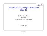
Task 3<br />
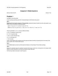
Add to the script in Task 2 to plot the location of airports in the State of Colorado. Use the usamap.mat file provided. Label your<br />
map as needed.<br />
___________ Matlab Script ___________<br />
% Script file for Task3 of <strong>Problem</strong> 2 (<strong>Assignment</strong> 7)<br />
matchAirportsCO=strcmp(state,'CO'); % finds indices of airports in Colorado<br />
index=find(matchAirportsCO==1);<br />
(optional step)<br />
latCO=latitude(index);<br />
longCO=longitude(index);<br />
% Extracts indices of airports in Colorado<br />
% Saves latitudes of airports in CO<br />
% Saves longitudes of airports in CO<br />
load usamap<br />
h=plot(uslon, uslat,'k-', longCO, latCO,'r *');<br />
xlabel('Longitude (deg)')<br />
ylabel('Latitude (deg)')<br />
grid<br />
___________________________________<br />
CEE 3804 Trani Page 8 of 9
Figure 2. U.S. Map with Airports in the State of Colorado.<br />
Task 4<br />
Find the total number of passengers boarding planes at airports in the state of Virginia.<br />
___________ Matlab Script ___________<br />
% Script file for Task 4 of <strong>Problem</strong> 2 (<strong>Assignment</strong> 7)<br />
matchAirportsVA=strcmp(state,'VA');<br />
indexVA=find(matchAirportsVA==1);<br />
% Finds indices of airports in VA<br />
% Extracts indices of airports in VA<br />
totalNumPssngr=sum(passengerPerYear(indexVA));<br />
disp(['Total Passengers at Airports in the State of Virginia ', num2str(totalNumPssngr) ])<br />
___________________________________<br />
Total Passengers at Airports in the State of Virginia 4,448,500.<br />
Note that IAD <strong>and</strong> DCA airports are considered to be in the District of Columbia for<br />
some strange reason in the database.<br />
CEE 3804 Trani Page 9 of 9