Using SPSS to Explore the IntroQuest Data File - Ecu
Using SPSS to Explore the IntroQuest Data File - Ecu
Using SPSS to Explore the IntroQuest Data File - Ecu

You also want an ePaper? Increase the reach of your titles
YUMPU automatically turns print PDFs into web optimized ePapers that Google loves.
<strong>Using</strong> <strong>SPSS</strong> <strong>to</strong> <strong>Explore</strong> <strong>the</strong> <strong>IntroQuest</strong> <strong>Data</strong> <strong>File</strong> <br />
This lesson teaches you how <strong>to</strong> use <strong>SPSS</strong> <strong>to</strong> explore a comma-delimited plain text data file.<br />
We shall use <strong>the</strong> INTROQ data file, which includes data collected from students in Dr. Wuensch’s<br />
undergraduate statistics classes from 1983 through this semester. Please read <strong>the</strong> document IntroQ<br />
Questionnaire <strong>to</strong> familiarize yourself with <strong>the</strong> variables on which we have data.<br />
Go <strong>to</strong> http://core.ecu.edu/psyc/wuenschk/Stat<strong>Data</strong>/Stat<strong>Data</strong>.htm and get <strong>the</strong><br />
<strong>IntroQuest</strong>.csv file (download it <strong>to</strong> your computer or portable medium). Each line of <strong>the</strong> data file has<br />
<strong>the</strong> data from one student. First comes <strong>the</strong> student's score on Gender (1 for female, 2 for male), <strong>the</strong>n<br />
a comma, <strong>the</strong>n <strong>the</strong> score on height (in inches) of each student’s Ideal mate, <strong>the</strong>n ano<strong>the</strong>r comma,<br />
<strong>the</strong>n Eye color (1 for brown, 2 for blue, 3 for green, and 4 for o<strong>the</strong>r), ano<strong>the</strong>r comma, Sta<strong>to</strong>phobia<br />
(fear of <strong>the</strong> course, on an 11 point scale, 0 through 10), comma, Nucophobia (subjective probability of<br />
nuclear war from 0% <strong>to</strong> 100%), comma, SATM (score on <strong>the</strong> math section of <strong>the</strong> Scholastic Aptitude<br />
Test), comma, and finally, Year <strong>the</strong> course was taken.<br />
If you were <strong>to</strong> open <strong>the</strong> INTROQ.csv file in a text edi<strong>to</strong>r, such as <strong>the</strong> Windows Notepad, <strong>the</strong><br />
first few lines would look like this:<br />
Gender,Ideal,Eye,Sta<strong>to</strong>ph,Nucoph,SATM,Year<br />
1,71,4,3,45,680,1983<br />
1,70,3,5,50,600,1983<br />
1,74,2,10,60,590,1983<br />
1,71,2,10,95,520,1983<br />
Notice that <strong>the</strong> variable names appear on <strong>the</strong> first line and <strong>the</strong> scores on <strong>the</strong> subsequent lines. A<br />
delimiter is <strong>the</strong> character used <strong>to</strong> separate one score from ano<strong>the</strong>r, so this is a comma delimited data<br />
file. “CSV” stands for “comma separated values.”<br />
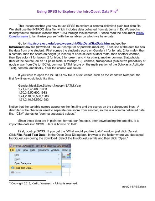
Since <strong>the</strong>se data are in plain text format, our first task, after downloading <strong>the</strong> data file, is <strong>to</strong><br />
import <strong>the</strong> data in<strong>to</strong> <strong>SPSS</strong>. Here is how <strong>to</strong> do that:<br />
First, boot up <strong>SPSS</strong>. If you get <strong>the</strong> "What would you like <strong>to</strong> do" window, just click Cancel.<br />
Click <strong>File</strong>, Read Text <strong>Data</strong>. In <strong>the</strong> Open <strong>Data</strong> Dialog box, browse <strong>to</strong> <strong>the</strong> folder where you deposited<br />
<strong>IntroQuest</strong>.csv during <strong>the</strong> download Select <strong>the</strong> <strong>IntroQuest</strong>.csv file and <strong>the</strong>n click “Open.”<br />
Copyright 2013, Karl L. Wuensch - All rights reserved.<br />
IntroQ1-<strong>SPSS</strong>.docx
2<br />
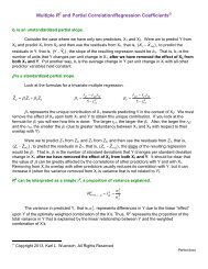
When you click “Open” <strong>the</strong> import Wizard pops up, like this:<br />
Tell it your text does not match a predefined format and <strong>the</strong>n click Next.
3<br />
Tell <strong>SPSS</strong> that <strong>the</strong> variables are DELIMITED (each value separated from <strong>the</strong> next by some<br />
special character) and that variable names are included at <strong>the</strong> <strong>to</strong>p of <strong>the</strong> file. Click Next.<br />
Tell <strong>SPSS</strong> that <strong>the</strong> data begin on line 2, each line represents a case, and you want <strong>to</strong> import all<br />
of <strong>the</strong> cases. Click Next.
4<br />
Tell <strong>SPSS</strong> that <strong>the</strong> delimiter is a comma, <strong>the</strong> text qualifier is None, and <strong>the</strong>n click Next.<br />
In Step 5, click each column and <strong>the</strong>n look above <strong>to</strong> be sure it is correctly identified as being a<br />
“Numeric” variable. Then click “Finish.” It will take you <strong>to</strong> Step 6. Just click “Finish” again.
5<br />
Click <strong>the</strong> “Variable View” tab in <strong>the</strong> <strong>Data</strong> Edi<strong>to</strong>r. Click in <strong>the</strong> Values column for <strong>the</strong> Gender<br />
variable. A little blue box with dots will appear on <strong>the</strong> right side of that cell – click it <strong>to</strong> get <strong>the</strong> Value<br />
Labels dialog window. In <strong>the</strong> Value field enter <strong>the</strong> number 1, hit tab, and in <strong>the</strong> Value Label field enter<br />
<strong>the</strong> word "Female" and <strong>the</strong>n click add. Now <strong>SPSS</strong> knows that those with value 1 for gender are<br />
women. Define <strong>the</strong> value 2 as "male" – do not forget <strong>to</strong> click Add after defining <strong>the</strong> value.<br />
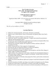
Click OK <strong>to</strong> end this process. Now define <strong>the</strong> labels for <strong>the</strong> Eye color variable (1 for brown, 2<br />
for blue, 3 for green, and 4 for o<strong>the</strong>r). The window should now look like this:
6<br />
If you look carefully at <strong>the</strong> data in <strong>the</strong> <strong>Data</strong> View, you will find that some cells contain only a<br />
period. These are cells for which <strong>the</strong> score is missing. For example, case number 27 in <strong>the</strong> CSV file<br />
appears like this: 1,62,3,9,50, ,1983. Notice that <strong>the</strong> next <strong>to</strong> last score is missing – <strong>the</strong>re is just a<br />
blank space between two commas where that score should be. This student could not remember e’s<br />
SAT Math score.<br />
The data are now ready <strong>to</strong> analyze, but first let us save <strong>the</strong> data in a <strong>SPSS</strong> format so that <strong>the</strong>y<br />
will be easier <strong>to</strong> bring back in<strong>to</strong> <strong>SPSS</strong> later, should we need <strong>the</strong>m later. Click <strong>File</strong>, Save As. Point at<br />
<strong>the</strong> folder where you want <strong>to</strong> save <strong>the</strong> file (if you are in a lab, point at your flash drive or Pirate Drive),<br />
give a file name of <strong>IntroQuest</strong>, and a file type of <strong>SPSS</strong>(*.sav). Click SAVE and <strong>the</strong> data are saved.<br />
Now we shall do some explora<strong>to</strong>ry data analysis. Click Analyze, Descriptive Statistics,<br />
<strong>Explore</strong>. Move Gender in<strong>to</strong> <strong>the</strong> Fac<strong>to</strong>r List. Move Ideal and Sta<strong>to</strong>ph in<strong>to</strong> <strong>the</strong> Dependent List.
Click Options and select “Exclude cases pairwise.” If you<br />
were <strong>to</strong> accept <strong>the</strong> default, “Exclude cases listwise,” <strong>SPSS</strong> would<br />
ignore all <strong>the</strong> data from any student who was missing a score on<br />
ei<strong>the</strong>r Ideal or Sta<strong>to</strong>ph. Sometimes we might want such listwise<br />
exclusion, but in this case we want <strong>SPSS</strong> <strong>to</strong> analyze all of <strong>the</strong><br />
available data on both of our variables. Continue, OK.<br />
7<br />
Look at <strong>the</strong> output. We have <strong>the</strong> basic statistics and plots <strong>to</strong><br />
compare <strong>the</strong> genders on height of ideal mate and fear of my<br />
statistics course. I find <strong>the</strong> schematic plots especially useful for visualizing such comparisons, but<br />
one should also look at <strong>the</strong> descriptive statistics. If you double click on <strong>the</strong> schematic plot, you enter<br />
<strong>the</strong> Chart Edi<strong>to</strong>r where you can modify various things, such as <strong>the</strong> colors and patterns used in <strong>the</strong><br />
plot.<br />
Now let us see if men and women differ with respect <strong>to</strong> what color <strong>the</strong>y report <strong>the</strong>ir eyes<br />
<strong>to</strong> be. Click Analyze, Descriptive Statistics, Crosstabs. Move gender in<strong>to</strong> <strong>the</strong> rows box and eye<br />
in<strong>to</strong> <strong>the</strong> columns box. Click Statistics, check Chi-Square, click Continue. Click Cells, check<br />
Observed Counts and Row Percentages, click Continue. Click OK.<br />
Look at <strong>the</strong> output. For <strong>the</strong> data as of May of 2013, <strong>the</strong> row percentages show us that women<br />
are more likely than men <strong>to</strong> report <strong>the</strong>ir eyes <strong>to</strong> be blue or green, while men are more likely than<br />
women <strong>to</strong> report <strong>the</strong>ir eyes <strong>to</strong> be brown or o<strong>the</strong>r – but <strong>the</strong> differences are quite small. Are <strong>the</strong><br />
differences in <strong>the</strong>se percentages large enough <strong>to</strong> convince us that in <strong>the</strong> population from which <strong>the</strong>se<br />
data were randomly sampled men and women differ with respect <strong>to</strong> how <strong>the</strong>y answer <strong>the</strong> eye color<br />
question The Chi-Square analysis helps us answer that question. In <strong>the</strong> row “Pearson Chi-<br />
Square,” column “Asymp. Sig,” you get a value known as <strong>the</strong> exact significance level, or p value.<br />
This is <strong>the</strong> probability of getting a sample with differences between men and women as large (or<br />
larger) than those we got if, in fact, <strong>the</strong>re were absolutely no differences between men and women<br />
(with respect <strong>to</strong> eye color) in <strong>the</strong> population. For <strong>the</strong> data as of May, 2013, that probability was .41.<br />
In o<strong>the</strong>r words, we would be quite likely <strong>to</strong> get data like those in our sample if in <strong>the</strong> population <strong>the</strong>re<br />
were no differences between men and women. Accordingly, we conclude that <strong>the</strong>re are no<br />
differences between men and women on this variable, or, if <strong>the</strong>re are, <strong>the</strong>y are really small. By<br />
convention, our p value has <strong>to</strong> come out <strong>to</strong> be .05 or less before we are convinced that <strong>the</strong><br />
differences found in our sample also exist in <strong>the</strong> population.
Now let’s look at some correlations between variables. Click Analyze, Correlate, Bivariate.<br />
Move every variable, except Eye, in<strong>to</strong> <strong>the</strong> Variables box. Select Pearson Correlation Coefficients,<br />
Two-Tailed, Flag Significant Correlations. Click OK.<br />
8<br />
Look at <strong>the</strong> output. For each pair of variables we are given a value of <strong>the</strong> correlation<br />
coefficient and <strong>the</strong> p value. Those with a p value of .05 or less are flagged as "significant," which just<br />
means that <strong>the</strong> evidence is good that those two variables are correlated in <strong>the</strong> population – that is, as<br />
<strong>the</strong> value of <strong>the</strong> one variable changes, <strong>the</strong> values of <strong>the</strong> o<strong>the</strong>r variable changes <strong>to</strong>o. Correlation<br />
coefficients range from –1 <strong>to</strong> +1. Values close <strong>to</strong> 0 indicate no association between <strong>the</strong> variables.<br />
Absolute values close <strong>to</strong> 1 indicate very strong association between <strong>the</strong> variables. A positive<br />
coefficient means that as <strong>the</strong> values of <strong>the</strong> one variable increase, so do <strong>the</strong> values of <strong>the</strong> o<strong>the</strong>r<br />
variable. A negative coefficient means that as values of <strong>the</strong> one variable increase, values of <strong>the</strong> o<strong>the</strong>r<br />
variable decrease.<br />
For <strong>the</strong> data as of May of 2013, <strong>the</strong> strongest correlation is between gender and ideal. Our<br />
sample data provide strong evidence that <strong>the</strong> average height of <strong>the</strong> ideal mates of men is smaller<br />
than <strong>the</strong> average height of <strong>the</strong> ideal mates of women – not a surprising finding. The correlation<br />
coefficient is negative because we coded female as 1 and male as 2, so as <strong>the</strong> code for gender went<br />
up, <strong>the</strong> value of height of ideal mate went down. Look at <strong>the</strong> correlation between height of ideal mate<br />
and sta<strong>to</strong>phobia. It indicates that students with taller ideal mates express greater fear of statistics.<br />
Can you explain this correlation<br />
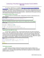
Finally, let us see how nucophobia has changed across<br />
<strong>the</strong> years. Click Graphs, Legacy Dialogs, Line, Simple,<br />
Summaries for Groups of Cases.
Click Define. Select “O<strong>the</strong>r Statistic (e.g., mean).” Scoot Nucoph in<strong>to</strong> <strong>the</strong> “Variable” box and<br />
Year in<strong>to</strong> <strong>the</strong> “Category Axis” box. OK.<br />
9<br />
Saving Your Statistical Output – very important<br />
After finishing your analysis, you should save your output so you can refer <strong>to</strong> it later. With <strong>the</strong><br />
Output window open, click <strong>File</strong>, Save.<br />
I recommend changing <strong>the</strong> name of <strong>the</strong> file from “Output” <strong>to</strong> something more descriptive, such<br />
as “IntroQ_Output.” It will be saved with <strong>the</strong> file extension “.spv.” You can open it later simply by<br />
double-clicking it in <strong>the</strong> folder. Output saved in this fashion can only be opened by <strong>SPSS</strong>.<br />
Still in <strong>the</strong> Output window, click <strong>File</strong>, Export, select <strong>the</strong> format you desire, browse <strong>to</strong> <strong>the</strong><br />
desired folder, name <strong>the</strong> output file, and click OK. The output file will likely contain a lot of stuff you<br />
will want <strong>to</strong> delete later, such as tables with info of no interest.
10<br />
If you are working in a lab, be sure that you save your work <strong>to</strong> a flash drive or <strong>to</strong> your Pirate<br />
Drive. If you save it <strong>to</strong> <strong>the</strong> hard drive, it may well not be <strong>the</strong>re when you need it later.<br />
Return <strong>to</strong> Wuensch’s <strong>SPSS</strong> Lessons Page<br />
Copyright 2013, Karl L. Wuensch - All rights reserved.