Astronomical Spectroscopy - Physics - University of Cincinnati

Astronomical Spectroscopy
Philip Massey
Lowell Observatory, 1400 W Mars Hill Road, Flagstaff, AZ 86001, USA;
phil.massey@lowell.edu
and
Margaret M. Hanson
Department of Physics, University of Cincinnati, PO Box 210011, Cincinnati, OH
45221-0011
ABSTRACT
Spectroscopy is one of the most important tools that an astronomer has for
studying the universe. This chapter begins by discussing the basics, including
the different types of optical spectrographs, with extension to the ultraviolet and
the near-infrared. Emphasis is given to the fundamentals of how spectrographs
are used, and the trade-offs involved in designing an observational experiment. It
then covers observing and reduction techniques, noting that some of the standard
practices of flat-fielding often actually degrade the quality of the data rather than
improve it. Although the focus is on point sources, spatially resolved spectroscopy
of extended sources is also briefly discussed. Discussion of differential extinction,
the impact of crowding, multi-object techniques, optimal extractions, flat-fielding
considerations, and determining radial velocities and velocity dispersions provide
the spectroscopist with the fundamentals needed to obtain the best data. Finally
the chapter combines the previous material by providing some examples of reallife
observing experiences with several typical instruments.
Index Terms and Key Words: collimator, differential refraction, flat fielding, biases,
gratings, Hydra, IMACS, MagE, STIS, OSIRIS, integral field spectroscopy, optimal extraction,
slit, spectrographs, coude, echelle, fibers, long-slit, near infrared, spectrophotometry,
spectroscopy

– 2 –
1. Introduction
They’re light years away, man, and that’s pretty far
(lightspeed’s the limit, the big speed limit)
But there’s plenty we can learn from the light of a star
(split it with a prism, there’s little lines in it)
–Doppler Shifting, Alan Smale (AstroCappella 1 )
Spectroscopy is one of the fundamental tools at an astronomer’s disposal, allowing one
to determine the chemical compositions, physical properties, and radial velocities of astronomical
sources. Spectroscopy is the means used to measure the dark matter content of
galaxies, the masses of two stars in orbit about each other, the mass of a cluster of galaxies,
the rate of expansion of the Universe, or discover an exoplanet around other stars, all using
the Doppler shift. It makes it possible for the astronomer to determine the physical conditions
in distant stars and nebulae, including the chemical composition and temperatures, by
quantitative analysis of the strengths of spectral features, thus constraining models of chemical
enrichment in galaxies and the evolution of the universe. As one well-known astronomer
put it, “You can’t do astrophysics just by taking pictures through little colored pieces of
glass,” contrasting the power of astronomical spectroscopy with that of broad-band imaging.
Everyone who has seen a rainbow has seen the light of the sun dispersed into a spectrum,
but it was Isaac Newton (1643-1727) who first showed that sunlight could be dispersed into
a continuous series of colors using a prism. Joseph von Fraunhofer (1787-1826) extended
this work by discovering and characterizing the dark bands evident in the sun’s spectrum
when sufficiently dispersed. The explanation of these dark bands was not understood until
the work of Gustav Kirchhoff (1824-1887) and Robert Bunsen (1811-1899), who proposed
that they were due to the selective absorption of a continuous spectrum produced by the hot
interior of the sun by cooler gases at the surface. The spectra of stars were first observed
visually by Fraunhofer and Angelo Secchi (1818-1878), either of whom may be credited with
having founded the science of astronomical spectroscopy.
The current chapter will emphasize observing and reduction techniques primarily for
optical spectroscopy obtained with charge coupled devices (CCDs) and the techniques needed
for near-infrared (NIR) spectroscopy obtained with their more finicky arrays. Spectroscopy
in the ultraviolet (UV) will also be briefly discussed. Very different techniques are required
for gamma-ray, x-ray, and radio spectroscopy, and these topics will not be included here.
1 http://www.astrocappella.com/

– 3 –
Similarly the emphasis here will be primarily on stellar (point) sources, but with some
discussion of how to extend these techniques to extended sources.
The subject of astronomical spectroscopy has received a rich treatment in the literature.
The volume on Astronomical Techniques in the original Stars and Stellar Systems series
contains a number of seminal treatments of spectroscopy. In particular, the introduction to
spectrographs by Bowen (1962) remains useful even 50 years later, as the fundamental physics
remains the same even though photographic plates have given way to CCDs as detectors.
The book on diffraction gratings by Loewen & Popov (1997) is also a valuable resource.
Grey (1976) and Schroeder (1974) provide very accessible descriptions of astronomical spectrographs,
while the “how to” guide by Wagner (1992) has also proven to be very useful.
Similarly the monograph by Walker (1987) delves into the field of astronomical spectroscopy
in a more comprehensive manner than is possible in a single chapter, and is recommended.
2. An Introduction to Astronomical Spectrographs
This section will concentrate on the hardware aspect of astronomical spectroscopy. The
basics are discussed first. The following subsections then describe specific types of astronomical
spectrographs, citing examples in current operation.
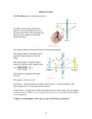
2.1. The Basics
When the first author was an undergraduate, his astronomical techniques professor,
one Maarten Schmidt, drew a schematic diagram of a spectrograph on the blackboard,
and said that all astronomical spectrographs contained these essential elements: a slit on
to which the light from the telescope would be focused; a collimator, which would take
the diverging light beam and turn it into parallel light; a disperser (usually a reflection
grating); and a camera that would then focus the spectrum onto the detector. In the
subsequent 35 years of doing astronomical spectroscopy for a living, the first author has yet
to encounter a spectrograph that didn’t meet this description, at least in functionality. In a
multi-object fiber spectrometer, such as Hectospec on the MMT (Fabricant et al. 2005), the
slit is replaced with a series of fibers. In the case of an echelle, such as MagE on the Clay
6.5-m telescope (Marshall et al. 2008), prisms are inserted into the beam after the diffraction
grating to provide cross-dispersion. In the case of an objective-prism spectroscopy, the star
itself acts as a slit “and the Universe for a collimator” (Newall 1910; see also Bidelman 1966).
Nevertheless, this heuristic picture provides the reference for such variations, and a version

– 4 –
is reproduced here in Figure 1 in the hopes that it will prove equally useful to the reader.
slit
collimator
grating
camera
lens
detector
Fig. 1.— The essential components of an astronomical spectrograph.
The slit sits in the focal plane, and usually has an adjustable width w. The image of
the star (or galaxy or other object of interest) is focused onto the slit. The diverging beam
continues to the collimator, which has focal length L coll . The f-ratio of the collimator (its
focal length divided by its diameter) must match that of the telescope beam, and hence its
diameter has to be larger the further away it is from the slit, as the light from a point source
should just fill the collimator. The collimator is usually an off-axis paraboloid, so that it
both turns the light parallel and redirects the light towards the disperser.
In most astronomical spectrographs the disperser is a grating, and is ruled with a certain
number of grooves per mm, usually of order 100-1000. If one were to place one’s eye near
where the camera is shown in Figure 1 the wavelength λ of light seen would depend upon
exactly what angle i the grating was set at relative to the incoming beam (the angle of
incidence), and the angle θ the eye made with the normal to the grating (the angle of
diffraction). How much one has to move one’s head by in order to change wavelengths by
a certain amount is called the dispersion, and generally speaking the greater the projected
number of grooves/mm (i.e., as seen along the light path), the higher the dispersion, all
other things being equal. The relationship governing all of this is called the grating equation
and is given as
mλ = σ(sin i + sin θ). (1)
In the grating equation, m is an integer representing the order in which the grating is
being used. Without moving one’s head, and in the absence of any order blocking filters, one

– 5 –
could see 8000Å light from first order and 4000Å light from second order at the same time 2 .
An eye would also have to see further into the red and blue than human eyes can manage,
but CCDs typically have sensitivity extending from 3000-10000Å, so this is a real issue, and
is solved by inserting a blocking filter into the beam that excludes unwanted orders, usually
right after the light has passed through the slit.
The angular spread (or dispersion 3 ) of a given order m with wavelength can be found
by differentiating the grating equation:
dθ/dλ = m/(σ cos θ) (2)
for a given angle of incidence i. Note, though, from Equation 1 that m/σ = (sin i+sin θ)/λ,
so
dθ/dλ = (sin i + sin θ)/(λ cosθ) (3)
In the Littrow condition (i = θ), the angular dispersion dθ/dλ is given by:
dθ/dλ = (2/λ) tanθ. (4)
Consider a conventional grating spectrograph. These must be used in low order (m is
typically 1 or 2) to avoid overlapping wavelengths from different orders, as discussed further
below. These spectrographs are designed to be used with a small angle of incidence, i.e., the
light comes into and leaves the grating almost normal to the grating) and the only way of
achieving high dispersion is by using a large number of groves per mm (i.e., σ is small in
Equation 2). (A practical limit is roughly 1800 grooves per mm, as beyond this polarization
effects limit the efficiency of the grating.) Note from the above that m/σ = 2 sin θ/λ in
the Littrow condition. So, if the angle of incidence is very low, tanθ ∼ sin θ ∼ θ, and the
angular dispersion dθ/dλ ∼ m/σ. If m must be small to avoid overlapping orders, then the
only way of increasing the dispersion is to decrease σ; i.e., use a larger number of grooves
per mm. Alternatively, if the angle of incidence is very high, one can achieve high dispersion
with a low number of groves per mm by operating in a high order. This is indeed how echelle
spectrographs are designed to work, with typically tanθ ∼ 2 or greater. A typical echelle
grating might have ∼ 80 grooves/mm, so, σ ∼ 25λ or so for visible light. The order m must
be of order 50. Echelle spectrographs can get away with this because they cross-disperse
2 This is because of the basics of interference: if the extra path length is any integer multiple of a given
wavelength, constructive interference occurs.
3 Although we derive the true dispersion here, the characteristics of a grating used in a particular spectrograph
usually describe this quantity in terms of the “reciprocal dispersion”, i.e., a certain number of Å per
mm or Å per pixel. Confusingly, some refer to this as the dispersion rather than the reciprocal dispersion.

– 6 –
the light (as discussed more below) and thus do not have to be operated in a particular low
order to avoid overlap.
Gratings have a blaze angle that results in their having maximum efficiency for a particular
value of mλ. Think of the grating as having little triangular facets, so that if one
is looking at the grating perpendicular to the facets, each will act like a tiny mirror. It
is easy to to envision the efficiency being greater in this geometry. When speaking of the
corresponding blaze wavelength, m = 1 is assumed. When the blaze wavelength is centered,
the angle θ above is this blaze angle. The blaze wavelength is typically computed for the
Littrow configuration, but that is seldom the case for astronomical spectrographs, so the
effective blaze wavelength is usually a bit different.
As one moves away from the blaze wavelength λ b , gratings fall to 50% of their peak
efficiency at a wavelength
λ = λ b /m − λ b /3m 2 (5)
on the blue side and
λ = λ b /m + λ b /2m 2 (6)
on the red side 4 . Thus the efficiency falls off faster to the blue than to the red, and the useful
wavelength range is smaller for higher orders. Each spectrograph usually offers a variety of
gratings from which to choose. The selected grating can then be tilted, adjusting the central
wavelength.
The light then enters the camera, which has a focal length of L cam . The camera takes
the dispersed light, and focuses it on the CCD, which is assumed to have a pixel size p,
usually 15µm or so. The camera design often dominates in the overall efficiency of most
spectrographs.
Consider the trade-off involved in designing a spectrograph. On the one hand, one
would like to use a wide enough slit to include most of the light of a point source, i.e., be
comparable or larger than the seeing disk. But the wider the slit, the poorer the spectral
resolution, if all other components are held constant. Spectrographs are designed so that
when the slit width is some reasonable match to the seeing (1-arsec, say) then the projected
slit width on the detector corresponds to at least 2.0 pixels in order to satisfy the tenet of
the Nyquist-Shannon sampling theorem. The magnification factor of the spectrograph is the
4 The actual efficiency is very complicated to calculate, as it depends upon blaze angle, polarization, and
diffraction angle. See Miller & Friedman (2003) and references therein for more discussion. Equations 5 and
6 are a modified version of the “2/3-3/2 rule” used to describe the cut-off of a first-order grating as 2/3λ b
and 3/2λ b ; see Al-Azzawi (2007).

– 7 –
ratio of the focal lengths of the camera and the collimator, i.e., L cam /L coll . This is a good
approximation if all of the angles in the spectrograph are small, but if the collimator-tocamera
angle is greater than about 15 degrees one should include a factor of r, the “grating
anamorphic demagnification”, where r = cos(t + φ/2)/cos(t − φ/2), where t is the grating
tilt and φ is collimator-camera angle (Schweizer 1979) 5 . Thus the projected size of the slit
on the detector will be WrL cam /L coll , where W is the slit width. This projected size should
be equal to at least 2 pixels, and preferably 3 pixels.
The spectral resolution is characterized as R = λ/∆λ, where ∆λ is the resolution element,
the difference in wavelength between two equally strong (intrinsically skinny) spectral
lines that can be resolved, corresponding to the projected slit width in wavelength units.
Values of a few thousand are considered “moderate resolution”, while values of several tens
of thousands are described as “high resolution”. For comparison, broad-band filter imaging
has a resolution in the single digits, while most interference-filter imaging has an R ∼ 100.
The free spectral range δλ is the difference between two wavelengths λ m and λ (m+1) in
successive orders for a given angle θ:
δλ = λ m − λ m+1 = λ m+1 /m. (7)
For conventional spectrographs that work in low order (m=1-3) the free spectral range is
large, and blocking filters are needed to restrict the observation to a particular order. For
echelle spectrographs, m is large (m ≥ 5) and the free spectral range is small, and the orders
must be cross-dispersed to prevent overlap.
Real spectrographs do differ in some regards from the simple heuristic description here.
For example, the collimator for a conventional long-slit spectrograph must have a diameter
that is larger than would be needed just for the on-axis beam for a point source, because it
has to efficiently accept the light from each end of the slit as well as the center. One would
like the exit pupil of the telescope imaged onto the grating, so that small inconsistencies in
guiding etc will minimize how much the beam “walks about” on the grating. An off-axis
paraboloid can do this rather well, but only if the geometry of the rest of the system matches
it rather well.
5 Note that some observing manuals give the reciprocal of r. As defined here, r ≤ 1.

– 8 –
2.1.1. Selecting a Blocking Filter
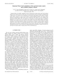
There is often confusion over the use of order separation filters. Figure 2 shows the
potential problem. Imagine trying to observe from 6000Å to 8000Å in first order. At this
particular angle, one will encounter overlapping light from 3000Å to 4000Å in second order,
and, in principle, 2000Å to 2666Å in third order, etc.
Since the atmosphere transmits very little light below 3000Å, there is no need to worry
about third or higher orders. However, light from 3000-4000Å does have to be filtered out.
There are usually a wide variety of blue cut-off filters to choose among; these cut off the
light in the blue but pass all the light longer than a particular wavelength. In this example,
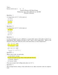
any cut-off filter that passed 6000Å and higher would be fine. The transmission curves of
some typical order blocking filters are shown in Figure 3. The reader will see that there are
a number of good choices, and that either a GG455, GG475, GG495, OG530, or an OG570
filter could be used. The GG420 might work, but it looks as if it is still passing some light
at 4000Å, so why take the chance
What if instead one wanted to observe from 4000Å to 5000Å in second order Then
there is an issue about first order red light contaminating the spectrum, from 8000Å on.
Third order light might not be a problem—at most there would be a little 3333Å light at
5000Å, but one could trust the source to be faint there and for the atmosphere to take its toll.
So, a good choice for a blocking filter would seem be a CuSO 4 filter. However, one should
be relatively cautious though in counting on the atmosphere to exclude light. Even though
many astronomers would argue that the atmosphere doesn’t transmit “much” in the near-
UV, it is worth noting that actual extinction at 3200Å is typically only about 1 magnitude
per airmass, and is 0.7 mag/airmass at 3400Å. So, in this example if one were using a very
blue spectrophotometric standard to flux calibrate the data, one could only count on its
second-order flux at 3333Å being attenuated by a factor of 2 (from the atmosphere) and
another factor of 1.5 (from the higher dispersion of third order). One might be better off
using a BG-39 filter (Figure 3).
One can certainly find situations for which no available filter will do the job. If instead
one had wanted to observe from 4000Å to 6000Å in second order, one would have such a
problem: not only does the astronomer now have to worry about >8000Å light from first
order, but also about

– 9 –
Fig. 2.— The overlap of various orders is shown.

– 10 –
Fig. 3.— Examples of the transmission curves of order blocking filters, taken from Massey
et al. (2000).

– 11 –
2.1.2. Choosing a grating
What drives the choice of one grating over another There usually needs to be some
minimal spectral resolution, and some minimal wavelength coverage. For a given detector
these two may be in conflict; i.e., if there are only 2000 pixels and a minimum (3-pixel)
resolution of 2Å is needed, then no more than about 1300Å can be covered in a single
exposure. The larger the number of lines per mm, the higher the dispersion (and hence
resolution) for a given order. Usually the observer also has in mind a specific wavelength
region, e.g., 4000Å to 5000Å. There may still be various choices to be made. For instance, a
1200 line/mm grating blazed at 4000Å and a 600 line/mm grating blazed at 8000Å may be
(almost) equally good for such a project, as the 600 line/mm could be used in second order
and will then have the same dispersion and effective blaze as the 1200 line grating. The
primary difference is that the efficiency will fall off much faster for the 600 line/mm grating
used in second order. As stated above (Equations 5 and 6), gratings fall off to 50% of their
peak efficiency at roughly λ b /m −λ b /3 2 and λ b /m+λ b /2m 2 where λ b is the first-order blaze
wavelength and m is the order. So, the 4000Å blazed 1200 line/mm grating used in first
order will fall to 50% by roughly 6000Å. However, the 8000Å blazed 600 line/mm grating
used in second order will fall to 50% by 5000Å. Thus most likely the first order grating
would be a better choice, although one should check the efficiency curves for the specific
gratings (if such are available) to make sure one is making the right choice. Furthermore, it
would be easy to block unwanted light if one were operating in second order in this example,
but generally it is a lot easier to perform blocking when one is operating in first order, as
described above.
2.2. Conventional Long-Slit Spectrographs
Most of what has been discussed so far corresponds to a conventional long-slit spectrograph,
the simplest type of astronomical spectrograph, and in some ways the most versatile.
The spectrograph can be used to take spectra of a bright star or a faint quasar, and the
long-slit offers the capability of excellent sky subtraction. Alternatively the long-slit can
be used to obtain spatially resolved spectra of extended sources, such as galaxies (enabling
kinematic, abundance, and population studies) or HII regions. They are usually easy to use,
with straightforward acquisition using a TV imaging the slit, although in some cases (e.g.,
IMACS on Magellan, discussed below in § 2.4.1) the situation is more complicated.
Table 1 provides characteristics for a number of commonly used long-slit spectrographs.
Note that the resolutions are given for a 1-arcsec wide slit.

– 12 –
Table 1. Some Long Slit Optical Spectrographs
Instrument Telescope Slit Slit scale R Comments
length (arcsec/pixel)
LRIS Keck I 2.9’ 0.14 500-3000 Also multi-slits
GMOS Gemini-N,S 5.5’ 0.07 300-3000 Also multi-slit masks
IMACS Magellan I 27’ 0.20 500-1200 f/2.5 camera, also multi-slit masks
15’ 0.11 300-5000 f/4 camera, also multi-slit masks
Goodman SOAR 4.2-m 3.9’ 0.15 700-3000 also multi-slit masks
RCSpec KPNO 4-m 5.4’ 0.7 300-3000
RCSpec CTIO 4-m 5.4’ 0.5 300-3000
STIS HST 0.9’ 0.05 500-17500
GoldCam KPNO 2.1-m 5.2’ 0.8 500-4000
RCSpec CTIO 1.5-m 7.5’ 1.3 300-3000
2.2.1. An Example: The Kitt Peak RC Spectrograph
Among the classic workhorse instruments of the Kitt Peak and Cerro Tololo Observatories
have been the Ritchey-Chretien (RC) spectrographs on the Mayall and Blanco 4-meter
telescopes. Originally designed in the era of photographic plates, these instruments were
subsequently outfitted with CCD cameras. The optical diagram for the Kitt Peak version
is shown in Figure 4. It is easy to relate this to the heuristic schematic of Figure 1. There
are a few additional features that make using the spectrograph practical. First, there is a
TV mounted to view the slit jaws, which are highly reflective on the front side. This makes
it easy to position an object onto the slit. The two filter bolts allow inserting either neutral
density filters or order blocking filters into the beam. A shutter within the spectrograph
controls the exposure length. The f/7.6 beam is turned into collimated (parallel) light by
the collimator mirror before striking the grating. The dispersed light then enters the camera,
which images the spectrum onto the CCD.
The “UV fast camera” used with the CCD has a focal length that provides an appropriate
magnification factor. The magnification of the spectrograph rL cam /L coll is 0.23r, with r
varying from 0.6 to 0.95, depending upon the grating. The CCD has 24µm pixels and thus
for 2.0 pixel resolution one can open the slit to 250µm, corresponding to 1.6 arcsec, a good
match to less than perfect seeing.
The spectrograph has 12 available gratings to choose among, and their properties are
given in Table 2.

– 13 –
4-Meter Telescope - RC Spectrograph
Optical Diagram
slit viewing TV
spectrograph
mounting surface
reflective slit jaws
grating
upper / lower
filter bolts
dispersed beam
shutter
UV-Fast
camera
CCD
collimator mirror
Fig. 4.— The optical layout of the Kitt Peak 4-meter RC Spectrograph. This figure is based
upon an illustration from the Kitt Peak instrument manual by James DeVeny.

– 14 –
Table 2. 4-m RC Spectrograph Gratings
Reciprocal
Name l/mm order Blaze Coverage(Å) Dispersion Resolution a
(Å) 1500 pixels 1700 pixels (Å/pixel) (Å)
BL 250 158 1 4000 1 octave b 5.52 13.8
BL 400 158 1 7000 1 octave b 5.52 13.8
2 3500

– 15 –
gratings blazed at the red. One could do well with KPC-22B (1st order blaze at 8500Å) with
a reciprocal dispersion of 1.44Å per pixel. One would have to employ some sort of blocking
filter to block the blue 2nd order light, with the choice dictated by exactly how the Ca II
triplet was centered within the 2450Å wavelength coverage that the grating would provide.
The blue spectrum can then be obtained by just changing the blocking filter to block 1st
order red while allowing in 2nd order blue. The blue 1200Å coverage would be just right
for covering the MK classification region from 3800-5000Å. By just changing the blocking
filter, one would then obtain coverage in the red from 7600Å to 1µm, with the Ca II lines
relatively well centered. An OG-530 blocking filter would be a good choice for the 1st order
red observations. For the 2nd order blue, either the BG-39 or CuSO 4 blocking filters would
be a good choice as either would filter out light with a wavelength of >7600, as shown in
Figure 3 6 . The advantage to this set up would be that by just moving the filter bolt from
one position to another one could observe in either wavelength region.
2.3. Echelle Spectrographs
In the above sections the issue of order separation for conventional slit spectrographs
have been discussed extensively. Such spectrographs image a single order at a given time.
On a large two-dimensional array most of the area is “wasted” with the spectrum of the
night sky, unless one is observing an extended object, or unless the slit spectrograph is used
with a multi-object slit mask, as described below.
Echelle spectrographs use a second dispersing element (either a grating or a prism) to
cross disperse the various orders, spreading them across the detector. An example is shown
in Figure 5. The trade off with designing echelles and selecting a cross-dispersing grating
is to balance greater wavelength coverage, which would have adjacent orders crammed close
together, with the desire to have a “long” slit to assure good sky subtraction, which would
have adjacent orders more highly separated 7 .
Echelles are designed to work in higher orders (typically m ≥ 5) and both i and θ in the
6 The BG-38 also looks like it would do a good job, but careful inspection of the actual transmission
curve reveals that it has a significant red leak at wavelengths >9000Å. It’s a good idea to check the actual
numbers.
7 Note that some “conventional” near-IR spectrographs are cross dispersed in order to take advantage of
the fact that the JHK bands are coincidently centered one with the other in orders 5, 4, and 3 respectively
(i.e., 1.25µm, 1.65µm, and 2.2µm).

– 16 –
Fig. 5.— The spectral format of MagE on its detector. The various orders are shown, along
with the approximate central wavelength.
grating equation (§ 2.1) are large 8 . At the detector one obtains multiple orders side-by-side.
Recall from above that the wavelength difference δλ between successive orders at a given
angle (the free spectral range) will scale inversely with the order number (Equation 7). Thus
for low order numbers (large central wavelengths) the free spectral range will be larger.
The angular spread δθ of a single order will be δλdθ/dλ. Combining this with the
equation for the angular dispersion (Equation 4) then yields:
λ/σ cosθ = δλ(2/λ) tanθ,
and hence the wavelength covered in a single order will be
The angular spread of a single order will be
δλ = λ 2 /(2σ sin θ). (8)
∆θ = λ/(σ cosθ). (9)
Thus the number of angstroms covered in a single order will increase by the square
of the wavelength (Equation 8), while the length of each order increases only linearly with
8 Throughout this section the term ”echelle” is used to include the so-called echellette. Echellette gratings
have smaller blaze angles (tan θ ≤ 0.5) and are used in lower orders (m =5-20) than classical echelles
(tanθ ≥ 2, m =20-100.) However, both are cross-dispersed and provide higher dispersions than conventional
grating spectrographs.

– 17 –
each order (Equation 9). This is apparent from Figure 5, as the shorter wavelengths (higher
orders) span less of the chip. At lower orders the wavelength coverage actually exceeds the
length of the chip. Note that the same spectral feature may be found on adjacent orders,
but usually the blaze function is so steep that good signal is obtained for a feature in one
particular order. This can be seen for the very strong H and K Ca II lines apparent near the
center of order 16 and to the far right in order 15 in Figure 5.
If a grating is used as the cross disperser, then the separation between orders should
increase for lower order numbers (larger wavelengths) as gratings provide fairly linear dispersion
and the free spectral range is larger for lower order numbers. (There is more of a
difference in the wavelengths between adjacent orders and hence the orders will be more
spread out by a cross-dispersing grating.) However, Figure 5 shows that just the opposite
is true for MagE: the separation between adjacent orders actually decreases towards lower
order numbers. Why MagE uses prisms for cross-dispersing, and (unlike a grating) the
dispersion of a prism is greater in the blue than in the red. In the case of MagE the decrease
in dispersion towards larger wavelength (lower orders) for the cross-dispersing prisms more
than compensates for the increasing separation in wavelength between adjacent orders at
longer wavelengths.
Some echelle spectrographs are listed in Table 3. HIRES, UVES, and the KPNO 4-m
echelle have a variety of gratings and cross-dispersers available; most of the others provide
a fixed format but give nearly full wavelength coverage in the optical in a single exposure.
Table 3. Some Echelle Spectrographs
Instrument Telescope R (1 arcsec slit) Coverage(Å) Comments
HIRES Keck I 39,000 Variable
ESI Keck II 4,000 3900-11000 Fixed format
UVES VLT-UT2 40,000 Variable Two arms
MAESTRO MMT 28,000 3185-9850 Fixed format
MIKE Magellan II 25,000 3350-9500 Two arms
MagE Magellan II 4,100

– 18 –
in detail by Marshall et al. (2008). The optical layout is shown in Figure 6. Light from
the telescope is focused onto a slit, and the diverging beam is then collimated by a mirror.
Cross dispersion is provided by two prisms, the first of which is used in double pass mode,
while the second has a single pass. The echelle grating has 175 lines/mm and is used in a
quasi-Littrow configuration. The Echelle Spectrograph and Imager (ESI) used on Keck II
has a similar design (Sheinis et al. 2002). MagE has a fixed format and uses orders 6 to 20,
with central wavelengths of 9700Å to 3125Å, respectively.
Fig. 6.— The optical layout of MagE. Based upon Marshall et al. (2008).
The spectrograph is remarkable for its extremely high throughput and ease of operation.
The spectrograph was optimized for use in the blue, and the measured efficiency of the
instrument alone is >30% at 4100Å. (Including the telescope the efficiency is about 20%.)
Even at the shortest wavelengths (3200Å and below) the overall efficiency is 10%. The
greatest challenge in using the instrument is the difficulties of flat-fielding over that large
a wavelength range. This is typically done using a combination of in- and out-of-focus Xe
lamps to provide sufficient flux in the near ultra-violet, and quartz lamps to provide good
counts in the red. Some users have found that the chip is sufficiently uniform that they do
better by not flat-fielding the data at all; in the case of very high signal-to-noise one can
dither along the slit. (This is discussed in general in § 3.2.6.) The slit length of MagE is 10
arcsec, allowing good sky subtraction for stellar sources, and still providing clean separation
between orders even at long wavelengths (Figure 5).
It is clear from an inspection of Figure 5 that there are significant challenges to the data
reduction: the orders are curved on the detector (due to the anamorphic distortions of the
prisms) and in addition the spectral features are also tilted, with a tilt that varies along each
order. One spectroscopic pundit has likened echelles to space-saving storage travel bags: a
lot of things are packed together very efficiently, but extracting the particular sweater one

– 19 –
wants can be a real challenge.
2.3.2. Coude Spectrographs
Older telescopes have equatorial mounts, as it was not practical to utilize an altitudeazimuth
(alt-az) design until modern computers were available. Although alt-az telescopes
allow for a more compact design (and hence a significant cost savings in construction of the
telescope enclosure), the equatorial systems provided the opportunity for a coude focus. By
adding three additional mirrors, one could direct the light down the stationary polar axis
of an equatorial system. From there the light could enter a large “coude room”, holding
a room-sized spectrograph that would be extremely stable. Coude spectrographs are still
in use at Kitt Peak National Observatory (fed by an auxiliary 0.9-m telescope), McDonald
Observatory (on the 2.7-m telescope), and at the Dominion Astrophysical Observatory (on
a 1.2-m telescope), among other places. Although such spectrographs occupy an entire
room, the basic idea was the same, and these instruments afford very high stability and high
dispersion. To some extent, these functions are now provided by high resolution instruments
mounted on the Nasmyth foci of large alt-az telescopes, although these platforms provide
relatively cramped quarters to achieve the same sort of stability and dispersions offered by
the classical coude spectrographs.
2.4. Multi-object Spectrometers
There are many instances where an astronomer would like to observe multiple objects
in the same field of view, such as studies of the stellar content of a nearby, resolved galaxy,
the members of a star cluster, or individual galaxies in a group. If the density of objects
is relatively high (tens of objects per square arcminute) and the field of view small (several
arcmins) then one often will use a slit mask containing not one but dozens or even hundreds
of slits. If instead the density of objects is relatively low (less than 10 per square arcminute)
but the field of view required is large (many arcmins) one can employ a multi-object fiber
positioner feeding a bench-mounted spectrograph. Each kind of device is discussed below.
2.4.1. Multi-slit Spectrographs
Several of the “long slit” spectrographs described in § 2.2 were really designed to be
used with multi-slit masks. These masks allow one to observe many objects at a time by

– 20 –
having small slitlets machined into a mask at specific locations. The design of these masks
can be quite challenging, as the slits cannot overlap spatially on the mask. An example is
shown in Figure 7. Note that in addition to slitlet masks, there are also small alignment holes
centered on modestly bright stars, in order to allow the rotation angle of the instrument and
the position of the telescope to be set exactly.
In practice, the slitlet masks need to be at least 5 arcsec in length in order to allow
sky subtraction on either side of a point source. Allowing for some small gap between the
slitlets, one can then take the field of view and divide by a typical slitlet length to estimate
the maximum number of slitlets an instrument would accommodate. Table 1 shows that an
instrument such as GMOS on the Gemini telescopes has a maximum (single) slit length of
5.5 arcmin, or 330 arcsec. Thus at most, one might be able to cram in 50 slitlets, were the
objects of interest properly aligned on the sky to permit this. An instrument with a larger
field of view, such as IMACS (described below) really excels in this game, as over a hundred
slitlets can be machined onto a single mask.
Multi-slit masks offer a large multiplexing advantage, but there are some disadvantages
as well. First, the masks typically need to be machined weeks ahead of time, so there is
really no flexibility at the telescope other than to change exposure times. Second, the setup
time for such masks is non-negligible, usually of order 15 or 20 minutes. This is not an
issue when exposure times are long, but can be a problem if the objects are bright and
the exposure times short. Third, and perhaps most significantly, the wavelength coverage
will vary from slitlet to slitlet, depending upon location within the field. As shown in the
example of Figure 7, the mask field has been rotated so that the slits extend north and
south, and indeed the body of the galaxy is mostly located north and south, minimizing
this problem. The alignment holes are located well to the east and west, but one does not
care about their wavelength coverage. In general, though, if one displaces a slit off center
by X arcsec, then the central wavelength of the spectrum associated with that slit is going
to shift by Dr(X/p), where p is the scale on the detector in terms of arcsec per pixel, r is
the anamorphic demagnification factor associated with this particular grating and tilt (≤1),
and D is the dispersion in Å per pixel.
Consider the case of the IMACS multi-object spectrograph. Its basic parameters are
included in Table 1, and the instrument is described in more detail below. The field of view
with the f/4 camera is 15 arcmins ×15 arcmins. A slit on the edge of the field of view will be
displaced by 7.5 arcmin, or 450 arcsec. With a scale of 0.11 arcsec/pixel this corresponds to
an offset of 4090 pixels (X/p = 4090). With a 1200 line/mm grating centered at 4500Å for a
slit on-axis, the wavelength coverage is 3700-5300Å with a dispersion D = 0.2Å/pixel. The
anamorphic demagnification is 0.77. So, for a slit on the edge the wavelengths are shifted

– 21 –
Fig. 7.— Multi-object mask of red supergiant candidates in NGC 6822. The upper left figure
shows an image of the Local Group galaxy NGC 6822, taken from the Local Group Galaxies
Survey (Massey et al. 2007). The red circles correspond to “alignment” stars, and the small
rectangles indicate the position of red supergiants candidates to be observed. The slit mask
consists of a large metal plate machined with these holes and slits. The upper right figure
is the mosaic of the 8 chips of IMACS. The vertical lines are night-sky emission lines, while
the spectra of individual stars are horizontal narrow lines. A sample of one such reduced
spectrum, of an M2 I star, is shown in the lower figure. These data were obtained by Emily
Levesque, who kindly provided parts of this figure.

– 22 –
by 630Å, and the spectrum is centered at 5130Å and covers 4330Å to 5930Å. On the other
edge the wavelengths will be shifted by -630Å, and will cover 3070Å to 4670Å. The only
wavelengths in common to slits covering the entire range in X is thus 4330Å-4670Å, only
340Å!
Example: IMACS The Inamori-Magellan Areal Camera & Spectrograph (IMACS) is a
innovative slit spectrograph attached to the Nasmyth focus of the Baade (Magellan I) 6.5-
m telescope (Dressler et al. 2006). The instrument can be used either for imaging or for
spectroscopy. Designed primarily for multi-object spectroscopy, the instrument is sometimes
used with a mask cut with a single long (26-inch length!) slit. There are two cameras, and
either is available to the observer at any time: an f/4 camera with a 15.4 arcmin coverage,
or an f/2.5 camera with a 27.5 arcmin coverage.
The f/4 camera is usable with any of 7 gratings, of which 3 may be mounted at any
time, and which provide resolutions of 300-5000 with a 1-arcsec wide slit. The delivered
image quality is often better than that (0.6 arcsec fwhm is not unusual) and so one can use
a narrower slit resulting in higher spectral resolution. The spectrograph is really designed
to take advantage of such good seeing, as a 1-arcsec wide slit projects to 9 unbinned pixels.
Thus binning is commonly used. The f/2.5 camera is used with a grism 9 , providing a longer
spatial coverage but lower dispersion. Up to two grisms can be inserted for use during a
night.
The optical design of the spectrograph is shown in Figure 8. Light from the f/11 focus of
the Baade Magellan telescope focuses onto the slit plate, enters a field lens, and is collimated
by transmission optics. The light is then either directed into the f/4 or f/2.5 camera. To
direct the light into the f/4 camera, either a mirror is inserted into the beam (for imaging)
or a diffraction grating is inserted (for spectroscopy). If the f/2.5 camera is used instead,
either the light enters directly (in imaging mode) or a transmission “grism” is inserted.
Each camera has its own mosaic of eight CCDs, providing 8192x8192 pixels. The f/4 camera
provides a smaller field of view but higher dispersion and plate scale; see Table 1. Pre-drilled
“long-slit” masks are available in a variety of slit widths. Up to six masks can be inserted
for a night’s observing, and selected by the instrument’s software.
9 A “grism” is a prism attached to a diffraction grating. The diffraction grating provides the dispersive
power, while the (weak) prism is used to displace the first-order spectrum back to the straight-on position.
The idea was introduced by Bowen & Vaughn (1973), and used successfully by Art Hoag at the prime focus
of the Kitt Peak 4-m telescope (Hoag 1976).

– 23 –
Fig. 8.— Optical layout of Magellan’s IMACS. This is based upon an illustration in the
IMACS user manual.
2.4.2. Fiber-fed Bench-Mounted Spectrographs
As an alternative to multi-slit masks, a spectrograph can be fed by multiple optical
fibers. The fibers can be arranged in the focal plane so that light from the objects of interest
enter the fibers, while at the spectrograph end the fibers are arranged in a line, with the
ends acting like the slit in the model of the basic spectrograph (Figure 1). Fibers were first
commonly used for multi-object spectroscopy in the 1980s, prior even to the advent of CCDs;
for example, the Boller and Chivens spectrograph on the Las Campanas du Pont 100-inch
telescope was used with a plug-board fiber system when the detector was an intensified
Reticon system. Plug-boards are like multi-slit masks in that there are a number of holes
pre-drilled at specific locations in which the fibers are then “plugged”. For most modern
fiber systems, the fibers are positioned robotically in the focal plane, although the Sloan
Digital Sky Survey used a plug-board system. A major advantage of a fiber system is that
the spectrograph can be mounted on a laboratory air-supported optical bench in a clean
room, and thus not suffer flexure as the telescope is moved. This can result in high stability,
needed for precision radial velocities. The fibers themselves provide additional “scrambling”
of the light, also significantly improving the radial velocity precision, as otherwise the exact
placement of a star on the slit may bias the measured velocities.
There are three down sides to fiber systems. First, the fibers themselves tend to have
significant losses of light at the slit end; i.e., not all of the light falling on the entrance

– 24 –
end of the fiber actually enters the fiber and makes it down to the spectrograph. These
losses can be as high as a factor of 3 or more compared to a conventional slit spectrograph.
Second, although typical fibers are 200-300µm in diameter, and project to a few arcsec on
the sky, each fiber must be surrounded by a protective sheath, resulting in a minimal spacing
between fibers of 20-40 arcsec. Third, and most importantly, sky subtraction is never “local”.
Instead, fibers are assigned to blank sky locations just like objects, and the accuracy of the
sky subtraction is dependent on how accurately one can remove the fiber-to-fiber transmission
variations by flat-fielding.
Table 4. Some Fiber Spectrographs
Instrument Telescope # Fiber size Closest FOV Setup R
fibers (µm) (”) spacing (arsec) (’) (mins)
Hectospec MMT 6.5-m 300 250 1.5 20 60 5 1000-2500
Hectochelle MMT 6.5-m 240 250 1.5 20 60 5 30,000
MIKE Clay 6.5-m 256 175 1.4 14.5 23 40 15,000-19,000
AAOMega AAT 4-m 392 140 2.1 35 120 65 1300-8000
Hydra-S CTIO 4-m 138 300 2.0 25 40 20 1000-2000
Hydra (blue) WIYN 3.5-m 83 310 3.1 37 60 20 1000-25000
Hydra (red) WIYN 3.5-m 90 200 2.0 37 50 20 1000-40000
An Example: Hectospec Hectospec is a 300-fiber spectrometer on the MMT 6.5-m
telescope on Mt Hopkins. The instrument is described in detail by Fabricant et al. (2005).
The focal surface consists of a 0.6-m diameter stainless steel plate onto which the magnetic
fiber buttons are placed by two positioning robots (Figure 9). The positioning speed of
the robots is unique among such instruments and is achieved without sacrificing positioning
accuracy (25µm, or 0.15 arcsec). The field of view is a degree across. The fibers subtend
1.5 arsec on the sky, and can be positioned to within 20 arcsec of each other. Light from
the fibers is then fed into a bench mounted spectrograph, which uses either a 270 line/mm
grating (R ∼ 1000) or a 600 line/mm grating (R ∼ 2500). The same fiber bundle can be
used with a separate spectrograph, known as Hectochelle.
Another unique aspect of Hectospec is the “cooperative” queue manner in which the
data are obtained, made possible in part because multi-object spectroscopy with fibers is
not very flexible and configurations are done well in advance of going to the telescope.
Observers are awarded a certain number of nights and scheduled on the telescope in the
classical way. The astronomers design their fiber configuration files in advance; these files
contain the necessary positioning information for the instrument, as well as exposure times,
grating setups, etc. All of the observations however become part of a collective pool. The

– 25 –
Fig. 9.— View of the focal plane of Hectospec. From Fabricant et al. (2005). Reproduced
by permission.
astronomer goes to the telescope on the scheduled night, but a “queue manager” decides on a
night-by-night basis which fields should be observed and when. The observer has discretion to
select alternative fields and vary exposure times depending upon weather conditions, seeing,
etc. The advantages of this over classical observing is that weather losses are spread amongst
all of the programs in the scheduling period (4 months). The advantages over normal queue
scheduled observations is that the astronomer is actually present for some of his/her own
observations, and there is no additional cost involved in hiring queue observers.
2.5. Extension to the UV and NIR
The general principles involved in the design of optical spectrographs extend to those
used to observe in the ultraviolet (UV) and near infrared (NIR), with some modifications.
CCDs have high efficiency in the visible region, but poor sensitivity at shorter ( 1µm) wavelengths. At very short wavelengths (x-rays, gamma-rays) and very long
wavelengths (mid-IR through radio and mm) special techniques are needed for spectroscopy,
and are beyond the scope of the present chapter.
Here we provide examples of two non-optical instruments, one whose domain is the

– 26 –
ultraviolet (1150-3200Å) and one whose domain is in the near infrared (1-2µm).
2.5.1. The Near Ultraviolet
For many years, astronomical ultraviolet spectroscopy was the purview of the privileged
few, mainly instrument Principle Investigators (PIs) who flew their instruments on highaltitude
balloons or short-lived rocket experiments. The Copernicus (Orbiting Astronomical
Observatory 3) was a longer-lived mission (1972-1981), but the observations were still PIdriven.
This all changed drastically due to the International Ultraviolet Explorer (IUE)
satellite, which operated from 1978-1996. Suddenly any astronomer could apply for time and
obtain fully reduced spectra in the ultraviolet. IUE’s primary was only 45 cm in diameter,
and there was considerable demand for the community to have UV spectroscopic capability
on the much larger (2.4-m) Hubble Space Telescope (HST).
The Space Telescope Imaging Spectrograph (STIS) is the spectroscopic work-horse of
HST, providing spectroscopy from the far-UV through the far-red part of the spectrum.
Although a CCD is used for the optical and far-red, another type of detector (multi-anode
microchannel array, or MAMA) is used for the UV. Yet, the demands are similar enough
for optical and UV spectroscopy that the rest of the spectrograph is in common to both the
UV and optical. The instrument is described in detail by Woodgate et al. (1998), and the
optical design is shown in Figure 10.
In the UV, STIS provides resolutions of ∼1000 to 10,000 with first-order gratings. With
the echelle gratings, resolution as high as 114,000 can be achieved. No blocking filters are
needed as the MAMA detectors are insensitive to longer wavelengths. From the point of
view of the astronomer who is well versed in optical spectroscopy, the use of STIS for UV
spectroscopy seems transparent.
With the success of the Servicing Mission 4 in May 2009, the Cosmic Origins Spectrograph
(COS) was added to HST’s suite of instruments. COS provides higher through
put than STIS (by factors of 10 to 30) in the far-UV, from 1100-1800Å. In the near-UV
(1700-3200Å) STIS continues to win out for many applications.
2.5.2. Near Infrared Spectroscopy and OSIRIS
Spectroscopy in the near-infrared (NIR) is complicated by the fact that the sky is much
brighter than most sources, plus the need to remove the strong telluric bands in the spectra.
In general, this is handled by moving a star along the slit on successive, short exposures

– 27 –
Fig. 10.— Optical design of STIS from Woodgate et al. (1998). Reproduced by permission.
(dithering), and subtracting adjacent frames, such that the sky obtained in the first exposure
is subtracted from the source in the second exposure, and the sky in the second exposure
is subtracted from the source in the first exposure. Nearly featureless stars are observed
at identical airmasses to that of the program object in order to remove the strong telluric
absorption bands. These issues will be discussed further in § 3.1.2 and § 3.3.3 below.
The differences in the basics of infrared arrays compared to optical CCDs also affect
how NIR astronomers go about their business. CCDs came into use in optical astronomy in
the 1980s because of their very high efficiency (≥50%, relative to photographic plates of a
few percent) and high linearity (i.e., the counts above bias are proportional to the number of
photons falling on their surface over a large dynamic range). CCDs work by exposing a thin
wafer of silicon to light and to collect the resulting freed charge carriers under electrodes.
By manipulating the voltages on those electrodes, the charge packets can be carried to a
corner of the detector array where a single amplifier can read them out successively. (The
architecture may also be used to feed multiple output amplifiers.) This allows for the creation
of a single, homogenous silicon structure for an optical array (see Mackay 1986 for a review).
For this and other reasons, optical CCDs are easily fabricated to remarkably large formats,
several thousand pixels to a side.
Things are not so easy in the infrared. The band gap (binding energy of the electron)
in silicon is simply too great to be dislodged by an infrared photon. For detection between 1

– 28 –
and 5 µm, either Mercury-Cadmium-Telluride (HgCdTe) or Indium-Antimonide (InSb) are
typically used, while the read out circuitry still remains silicon-based. From 5 to 28 µm,
silicon-based (extrinsic photoconductivity) detector technology is used, but they continue
to use similar approaches to array construction as in the near-infrared. The two layers
are joined electrically and mechanically with an array of Indium bumps. (Failures of this
Indium bond lead to dead pixels in the array.) Such a two-layered device is called a hybrid
array (Beckett 1995). For the silicon integrated circuitry, a CCD device could be (and was
originally) used, but the very cold temperatures required for the photon detection portion
of the array produced high read noise. Instead, an entirely new structure that provides a
dedicated readout amplifier for each pixel was developed (see Rieke 2007 for more details).
These direct read-out arrays are the standard for infrared instruments and allow for enormous
flexibility in how one reads the array. For instance, the array can be set to read the charge on
a specific, individual pixel without even removing the accumulated charge (non-destructive
read). Meanwhile, reading through a CCD removes the accumulated charge on virtually
every pixel on the array.
Infrared hybrid arrays have some disadvantages, too. Having the two components (detection
and readout) made of different materials limits the size of the array that can be
produced. This is due to the challenge of matching each detector to its readout circuitry to
high precision when flatly pressed together over millions of unit cells. Even more challenging
is the stress that develops from differential thermal contraction when the hybrid array is
chilled down to very cold operating temperatures. However, improvements in technology
now make it possible to fabricate 2K × 2K hybrid arrays, and it is expected that 4K × 4K
will eventually be possible. Historically, well depths have been lower in the infrared arrays,
though hybrid arrays can now be run with a higher gain. This allows for well depths approaching
that available to CCD arrays (hundreds of thousands of electrons per pixel). All
infrared hybrid arrays have a small degree of nonlinearity, of order a few percent, due to a
slow reduction in response as signals increase (Rieke 2007). In contrast, CCDs are typically
linear to a few tenths of a percent over five orders of magnitude. Finally, the infrared hybrid
arrays are far more expensive to build than CCDs. This is because of the extra processing
steps required in fabrication and their much smaller commercial market compared to CCDs.
The Ohio State Infrared Imager/Spectrometer (OSIRIS) provides an example of such
an instrument, and how the field has evolved over the past two decades. OSIRIS is a multimode
infrared imager and spectrometer designed and built by The Ohio State University
(Atwood et al. 1992, Depoy et al. 1993). Despite being originally built in 1990, it is still in
operation today, most recently spending several successful years at the Cerro Tololo Inter-
American Observatory Blanco 4-m telescope. Presently, OSIRIS sits at the Nasmyth focus
on the 4.1-m Southern Astrophysical Research (SOAR) Telescope on Cerro Pachón.

– 29 –
When built twenty years ago, the OSIRIS instrument was designed to illuminate the
best and largest infrared-sensitive arrays available at the time, the 256 x 256 pixel NICMOS3
HgCdTe arrays, with 27 µm pixels. This small array has long since been upgraded as infrared
detector technology has improved. The current array on OSIRIS is now 1024 x 1024 in size,
with 18.5 µm pixels (NICMOS4, still HgCdTe). As no design modifications could be afforded
to accommodate this upgrade, the larger array now used is not entirely illuminated due to
vignetting in the optical path. This is seen as a fall off in illumination near the outer corners
of the array.
OSIRIS provides two cameras, f/2.8 for lower resolution work (R ∼ 1200 with a 3.2-
arcmin long slit) and f/7 for higher-resolution work (R ∼ 3000, with a 1.2-arcminute long
slit). One then uses broad-band filters in the J (1.25 µm), H (1.65 µm) or K (2.20 µm) bands,
to select the desired order, 5th, 4th and 3rd, respectively. The instrument grating tilt is set
to simultaneously select the central regions of these three primary transmission bands of the
atmosphere. However, one can change the tilt to optimize observations at wavelengths near
the edges of these bands. OSIRIS does have a cross-dispersed mode, achieved by introducing
a cross-dispersing grism in the filter wheel. A final filter, which effectively blocks light outside
of the J, H, and K bands, is needed for this mode. The cross-dispersed mode allows observing
at low resolution (R ∼ 1200) in all three bands simultaneously, albeit it with a relatively
short slit (27-arcsecs).
Source acquisition in the infrared is not so straightforward. While many near-infrared
objects have optical counterparts, many others do not or show rather different morphology
or central positions offsets between the optical and infrared. This means acquisition and
alignment must be done in the infrared, too. OSIRIS, like most modern infrared spectrometers,
can image its own slit onto the science detector when the grating is not deployed in the
light path. This greatly facilitates placing objects on the slit (some NIR spectrometers have
a dedicated slit viewing imager so that objects may be seen through the slit during an actual
exposure). This quick-look imaging configuration is available with an imaging mask too,
and deploys a flat mirror in place of the grating (without changing the grating tilt) thereby
displaying an infrared image of the full field or slit with the current atmospheric filter. This
change in configuration only takes a few seconds and allows one to align the target on the
slit then quickly return the grating to begin observations. Even so, the mirror/grating flip
mechanism will only repeat to a fraction of a pixel when being moved to change between
acquisition and spectroscopy modes. The most accurate observations may then require new
flat fields and or lamp spectra be taken before returning to imaging (acquisition) mode.
For precise imaging observations, OSIRIS can be run in ”full” imaging mode which
includes placing a cold mask in the light path to block out-of-beam back ground emission

– 30 –
for the telescope primary and secondary. Deployment of the mask can take several minutes.
This true imaging mode is important in the K-band where background emission becomes
significant beyond 2µm due to the warm telescope and sky.
There are fantastic new capabilities for NIR spectroscopy about to become available as
modern multi-object spectrometers come on-line on large telescopes (LUCIFER on the Large
Binocular Telescope, MOSFIRE on Keck, FLAMINGOS-2 on Gemini-South, and MMIRS
on the Clay Magellan telescope). As with the optical, utilizing the multi-object capabilities
of these instruments effectively requires proportionately greater observer preparation, with
a significant increase in the complexity of obtaining the observations and performing the
reductions. Such multi-object NIR observations are not yet routine, and as such details are
not given here. One should perhaps master the “simple” NIR case first before tackling these
more complicated situations.
2.6. Spatially Resolved Spectroscopy of Extended Sources: Fabry-Perots and
Integral Field Spectroscopy
The instruments described above allow the astronomer to observe single or multiple
point sources at a time. If instead one wanted to obtain spatially resolved spectroscopy of a
galaxy or other extended source, one could place a long slit over the object at a particular
location and obtain a one-dimensional, spatially resolved spectrum. If one wanted to map
out the velocity structure of an HII region or galaxy, or measure how various spectral features
changed across the face of the object, one would have to take multiple spectra with the slit
rotated or moved across the object to build up a three dimensional image “data cube”: twodimensional
spatial location plus wavelength. Doing this is sometimes practical with a long
slit: one might take spectra of a galaxy at four different position angles, aligning the slit
along the major axis, the minor axis, and the two intermediate positions. These four spectra
would probably give a pretty good indication of the kinematics of the galaxy. But, if the
velocity field or ionization structure is complex, one would really want to build up a more
complete data cube. Doing so by stepping the slit by its width over the face of an extended
object would be one way, but clearly very costly in terms of telescope time.
An alternative would be to use a Fabry-Perot interferometer, basically a tunable filter.
A series of images through a narrow-band filter is taken, with the filter tuned to a slightly
different wavelength for each exposure. The resulting data are spatially resolved, with the
spectral resolution dependent upon the step size between adjacent wavelength settings. (A
value of 30 km s −1 is not atypical for a step size; i.e., a resolution of 10,000.) The wavelength
changes slowly as a function of radial position within the focal plane, and thus a “phase-

– 31 –
corrected” image cube is constructed which yields both an intensity map (such being a direct
image) and radial velocity map for a particular spectral line (for instance, Hα).
This works fine in the special case where one is interested in only a few spectral features
in an extended object. Otherwise, the issue of scanning spatially has simply been replaced
with the need to scan spectrally.
Alternative approaches broadly fall under the heading of integral field spectroscopy,
which simply means obtaining the full data cube in a single exposure. There are three
methods of achieving this, following Allington-Smith et al. (1998).
Lenslet arrays: One method of obtaining integral field spectroscopy is to place a microlens
array (MLA) at the focal plane. The MLA produces a series of images of the telescope
pupil, which enter the spectrograph and are dispersed. By tilting the MLA, one can arrange
it so that the spectra do not overlap with one another.
Fiber bundles: An array of optical fibers is placed in the focal plane, and the fibers then
transmit the light to the spectrograph, where they are arranged in a line, acting as a slit.
This is very similar to the use of multi-object fiber spectroscopy, except that the ends of the
fibers in the focal plane are always in the same configuration, with the fibers bundled as close
together as possible. There are of course gaps between the fibers, resulting in incomplete
spatial coverage without dithering.
It is common to use both lenslets and fibers together, as for instance is done with the
integral field unit of the FLAMES spectrograph on the VLT.
Image slicers: A series of mirrors can be used to break up the focal plane into congruent
“slices” and arrange these slices along the slit, analogous to a classic Bowen image slicer 10 .
One advantage of the image slicer technique for integral-field spectroscopy is that spatial
10 When observing an astronomical object, a narrow slit is needed to maintain good spectral resolution,
as detailed in § 2.1. Yet, the size of the image may be much larger than the size of the slit, resulting in
a significant loss of light, known as “slit losses”. Bowen (1938) first described a novel device for reducing
slit losses by changing the shape of the incoming image to match that of a long, narrow slit: a cylindrical
lens is used to slice up the image into a series of strips with a width equal to that of the slit, and then to
arrange them end to end along the slit. This needs to be accomplished without altering the focal ratio of
the incoming beam. Richardson et al. (1971) describes a variation of the same principle, while Pierce (1965)
provides detailed construction notes for such a device. The heyday of image slicers was in the photographic
era, where sky subtraction was impractical and most astronomical spectroscopy was not background limited.
Nevertheless, they have not completely fallen into disuse. For instance, GISMO (Gladders Image-Slicing
Multislit Option) is an image slicing device available for use with multi-slit plates on Magellan’s IMACS
(§ 2.4.1) to re-image the central 3.5 arcmin × 3.2 arcmin of the focal plane into the full field of view of the
instrument, allowing an 8-fold increase in the spatial density of slits.

– 32 –
information within the slice is preserved.
3. Observing and Reduction Techniques
This section will begin with a basic outline of how spectroscopic CCD data are reduced,
and then extend the treatment to the reduction of NIR data. Some occasionally overlooked
details will be discussed. The section will conclude by placing these together by describing a
few sample observing runs. It may seem a little backwards to start with the data reduction
rather than with the observing. But, only by understanding how to reduce data can one
really understand how to best take data.
The basic premise throughout this section is that one should neither observe nor reduce
data by rote. Simply subtracting biases because all of one’s colleagues subtract biases is an
inadequate reason for doing so. One needs to examine the particular data to see if doing so
helps or harms. Similarly, unless one is prepared to do a little math, one might do more harm
than good by flat-fielding. Software reduction packages, such as IRAF 11 or ESO-MIDAS 12
are extremely useful tools—in the right hands. But, one should never let the software provide
a guide to reducing data. Rather, the astronomer should do the guiding. One should strive
to understand the steps involved at the level that one could (in principle) reproduce the
results with a hand calculator!
In addition, there are very specialized data reduction pipelines, such as HST’s CALSTIS
and IMACS’s COSMOS, which may or may not do what is needed for a specific application.
The only way to tell is to try them, and compare the results with what one obtains by more
standard means. See § 3.2.5 for an example where the former does not do very well.
3.1. Basic Optical Reductions
The simplest reduction example involves obtaining a spectrum of a star obtained from
a long slit spectrograph. What calibration data does one need, and why
11 The Image Reduction and Analysis Facility is distributed by the National Optical Astronomy Observatory,
which is operated by the Association of Universities for Research in Astronomy, under cooperative
agreement with the National Science Foundation.
12 The European Southern Observatory Munich Image Data Analysis System

– 33 –
• The data frames themselves doubtless contain an overscan strip along the side, or
possibly along the top. As a CCD is read out, a “bias” is added to the data to assure
that no values go below zero. Typically this bias is several hundred or even several
thousand electrons (e − ) 13 . The exact value is likely to change slightly from exposure to
exposure, due to slight temperature variations of the CCD. The overscan value allows
one to remove this offset. In some cases the overscan should be used to remove a one
dimensional bias structure, as demonstrated below.
• Bias frames allow one to remove any residual bias structure. Most modern CCDs,
used with modern controllers, have very little (if any) bias structure, i.e., the bias
levels are spatially uniform across the chip. So, it’s not clear that one needs to use
bias frames. If one takes enough bias frames (9 or more) and averages them correctly,
one probably does very little damage to the data by using them. Still, in cases where
read-noise dominants your program spectrum, subtracting a bias could increase the
noise of the final spectrum.
• Bad pixel mask data allows one to interpolate over bad columns and other non-linear
pixels. These can be identified by comparing the average of a series of exposures of
high counts with the average of a series of exposures of low counts.
• Dark frames are exposures of comparable length to the program objects but obtained
with the shutter closed. In the olden days, some CCDs generated significant dark
current due to glowing amplifiers and the like. Dark frames obtained with modern
CCDs do little more than reveal light leaks if taken during daytime. Still, it is generally
harmless to obtain them.
• Featureless flats (usually “dome flats”) allow one to correct the pixel-to-pixel variations
within the detector. There have to be sufficient counts to not significantly degrade
the signal-to-noise ratio of the final spectrum. This will be discussed in more detail in
§ 3.2.6.
• Twilight flats are useful for removing any residual spatial illumination mismatch
between the featureless flat and the object exposure. This will be discussed in more
detail in § 3.2.6.
• Comparison arcs are needed to apply a wavelength scale to the data. These are
usually short exposures of a combination of discharge tubes containing helium, neon,
13 We use “counts” to mean what gets recorded in the image; sometimes these are also known as analog-todigital
units (ADUs). We use “electrons” (e − ) to mean the things that behave like Poisson statistics, with
the noise going as the square root of the number of electrons. The gain g is the number of e − per count.

– 34 –
and argon (HeNeAr), or thorium and argon (ThAr), with the choices dictated by what
lamps are available and the resolution. HeNeAr lamps are relatively sparse in lines and
useful at low to moderate dispersion; ThAr lamps are rich in lines and useful at high
dispersion, but have few unblended lines at low or moderate dispersions.
• Spectrophotometric standard stars are stars with smooth spectra with calibrated
fluxes used to determine the instrument response. Examples of such stars can be found
in Oke (1990), Stone (1977, 1996), Stone & Baldwin (1983), Massey et al. (1988, 1990),
and particularly Hamuy et al. (1994). Exposures should be long enough to obtain at
least 10,000 e − integrated over 50Å bandpass, i.e., at least 200 e − per Å integrated
over the spatial profile.
The basic reduction steps are described here. For convenience to the reader, reference is
made to the relevant IRAF tasks. Nevertheless, the goal is to explain the steps, not identify
what buttons need to be pushed.
1. Fit and subtract overscan. Typically the overscan occupies 20-40 columns on the
right side (high column numbers) of the chip. The simplest thing one can do is to
average the results of these columns on a row-by-row basis, and then fit these with a
low-order function, possibly a constant.
An example of such a nicely behaved overscan in shown in the left panel of Figure 11.
In other cases, there is a clear gradient in the bias section that should be removed by a
higher-order fit. The IMACS chips, for instance, have an overscan at both the top and
the right, and it is clear from inspection of the bias frames that the top overscan tracks
a turn-up on the left side. Such an overscan is shown in the middle panel of Figure 11.
Occasionally the overscan allows one to correct for some problem that occurred during
the read-out of the chip. For instance, the GoldCam spectrometer chip suffers 10-20
e − striping along rows if the controller electronics get a bit too hot. (This situation
is sometimes referred to as “banding”.) A similar problem may occur if there is radio
transmission from a nearby walkie-talkie during readout. However, these stripes extend
into the overscan, which can be used to eliminate them by subtracting the overscan
values in a row-by-row manner rather than by subtracting a low- or high-order function.
Such banding is shown in the right panel of Figure 11. In IRAF, overscan subtraction
is a task performed in the first pass through ccdproc.
2. Trim. Most spectroscopic data do not extend over the entire face of the chip, and
the blank areas will need to be trimmed off. Often the first or last couple of rows and
columns are not well behaved and should be trimmed as well. At the very least, the

– 35 –
Fig. 11.— Three examples of overscan structure. The overscan values have been averaged
over the 20-40 widths of the overscan region, and are shown plotted against the read-axis.
The overscan on the left is from the GoldCam spectrometer on the Kitt Peak 2.1-m and is
best fit by a constant value. The overscan in the middle is from chip 3 of IMACS, and shows
a pronounced upturn on the left, and is best fit with a low-order function. (Note too the
bad column around pixel 420.) The overscan on the right is also from GoldCam, but during
an electronics problem that introduced a number of bands with low values that were also in
the data region. Subtracting the average values in the overscan row-by-row removed them
to a good approximation.

– 36 –
overscan regions need to be removed. In IRAF this task is performed in the same step
as the overscan subtraction by ccdproc.
3. Dark subtraction. In the highly unlikely event that there is significant dark current
the dark frame should be subtracted from all of the images after scaling by the relevant
exposure times.
4. Interpolate over bad pixels. This step is mostly cosmetic, but is necessary if one
plans to flux-calibrate. Most CCDs have a few bad columns and non-linear pixels.
To identify these one can use two series of exposures of featureless flats: one of high
intensity level (but be careful not to saturate!) and one of low intensity. Enough of
these low-intensity flats need to be taken in order for the average to have a reasonable
signal-to-noise ratio. Typically 3 exposures of an internal quartz lamp (say) might be
taken, along with 50 frames of similar exposure time with a 100× attenuating neutral
density filter. The first series may contain 10,000 counts/pixel, while the latter only 100
counts/pixel. Averaging each series and dividing the results identifies the non-linear
pixels. One can construct a bad pixel “mask” (an image that is only a few bits deep)
to use to decide whether to interpolate along rows (in order to handle bad columns)
or over rows and columns (to handle isolated bad pixels), etc. The relevant tasks in
IRAF are ccdmask which generates a bad pixel mask, followed by using the mask in
ccdproc.
5. Construct (and use) a master bias frame. All the bias frames (which have been
treated by steps 1-2 as well) are combined and examined to see if there is any spatial
structure. If there is, then it is worth subtracting this master bias frame from all the
program frames. The relevant IRAF tasks are zerocombine and ccdproc.
6. Construct and apply a master normalized featureless flat. All of the dome flat
exposures are combined using a bad pixel rejection algorithm. The IRAF task for this
combination is flatcombine. The question then is how to best normalize the flat
Whether the final step in the reduction process is to flux-calibrate the spectrum, or
simply to normalize the spectrum to the continuum, the effort is going to be much
easier if one makes the correct choice as to how to best normalize the flat. Physically
the question comes down to whether or not the shape of the featureless flat in the
wavelength direction is dominated by the same effects as the astronomical object one
is trying to reduce, or if instead it is dominated by the calibration process. For instance,
all flats are likely to show some bumps and wiggles. Are the bumps and wiggles due
to the grating If so, one is better off fitting the flat with a constant value (or a
low order function) and using that as the flat’s normalization. That way the same

– 37 –
bumps and wiggles are present in both the program data as in the flat, and will divide
out. If instead some of the bumps and wiggles are due to filters in front of the flatfield
lamp, or the extreme difference in color temperature between the lamps and the
object of interest, or due to wavelength-dependent variations in the reflectivity of the
paint used for the flat-field screen, then one is better off fitting the bumps and wiggles
by using a very high order function, and using the flat only to remove pixel-to-pixel
variations. It usually isn’t obvious which will be better a priori, and really the only
thing to do is to select an object whose spectrum is expected to be smooth (such as a
spectrophotometric standard) and reduce it through the entire process using each kind
of flat. It will be easy to tell in the end. The IRAF task for handing the normalization
of the flat is response, and the flat field division is handled by ccdproc.
An example is shown in Figure 12. The flat-field has a very strong gradient in the
wavelength direction, and a bit of a bend around pixel 825 (about 4020Å). Will one do
better by just normalizing this by a constant value, ascribing the effects to the grating
and spectrograph Or should one normalize the flat with a higher order function
based on the assumption that these features are due to the flat-field system and very
red lamps (Blue is on the right and red is on the left.) The only way to answer the
question is to reduce some data both ways and compare the results, as in Figure 12.
The flat fit by a constant value does a better job removing both the gradient and the
bump. (The spectrum needs to be magnified to see that the bump at 4020Å has been
removed.) Thus the flat was a good reflection of what was going on in the spectrograph,
and is not due to issues with the calibration system.
Once one determines the correct normalized flat, it needs to be divided into all of the
data. The IRAF task for handling this is again ccdproc.
7. Construct and Use Illumination Function Correction. The non-uniformity in
the spatial direction is referred to as the “slit illumination function” and is a combination
of any unevenness in the slit jaws, the vignetting within the focal plane or within
the spectrograph, etc. Most of these issues should have been removed by dividing by
the flat field in step 6. Is this good enough If the remaining non-uniformity (relative
to the night sky) is just a few percent, and has a linear gradient, this is probably fine
for sky subtraction from a point source as one can linearly interpolate from the sky
values on either side of the object. However, if the remaining non-uniformity is peaked
or more complex, or if the goal is to measure the surface brightness of an extended
source, then getting the sky really and truly flat is crucial, and worth some effort.
The cheapest solution (in terms of telescope time) is to use exposures of the bright
twilight sky. With the telescope tracking, one obtains 3-5 unsaturated exposures,
moving the telescope slightly (perpendicular to the slit) between exposures. To use

– 38 –
Fig. 12.— Normalization of Flats. Left. The flat field counts varies by a factor of of 10 or
more with wavelength, and there is a discontinuity in the derivative around pixel 820. Middle.
Normalizing the flat by a constant yields a smooth stellar spectrum. Right. Normalizing the
flat by a higher order function results in an artificially large gradient in the counts.
these, one can combine the exposures (scaling each by the average counts), averaging
the spatial profile over all wavelengths, and then fitting a smooth function to the spatial
profile. The result is an image that is uniform along each row of the dispersion axis,
and hopefully matches the night sky perfectly in the spatial direction. Sadly this is
usually not the case, as during bright twilight there is light bouncing off of all sorts
of surfaces in the dome. Thus one might need to make a further correction using
exposures of the dark night sky itself. This process in illustrated in Figure 13. The
relevant IRAF tasks involved are imcombine, illumination, and ccdproc
This concludes the basic CCD reductions, and one is now ready to move on to extracting
and calibrating the spectrum itself.
8. Identification of Object and Sky. At this stage one needs to understand the
location of the stellar spectrum on the detector, decide how wide an extraction window
to use, and to select where the sky regions should be relative to the stellar spectrum.
The location of the star on the detector will doubtless be a mild function of wavelength,
due either to slight non-parallelism in how the grating is mounted or simply atmospheric
differential refraction. This map of the location of the stellar spectrum with wavelength
is often referred to as the “trace”. Examples are shown in Figure 14. In IRAF this is
done either as part of apall or via doslit.
9. Wavelength calibration. Having established the aperture and trace of the stellar
spectrum, it behooves one to extract the comparison spectrum in exactly the same
manner (i.e., using the same trace), and then identify the various lines and perform a
smooth fit to the wavelength as a function of pixel number along the trace. Figure 15

– 39 –
Fig. 13.— The spatial profile after flattening by the dome flat (step 6) is shown at the upper
left. Clearly there is a gradient from left to right. The profile of the twilight sky is shown
in the middle. It’s not a particularly good match, and after dividing by it we see that the
situation is not improved (top right). The profile of all of the sky exposures (after division
by the twilight profile) is shown at lower left, and was used to re-correct all of the data.
After this, the spatial profile was flatter, as shown at lower right, although there is now a
modest kink.

Counts
non-linear component (angstroms)
Counts
Line
– 40 –
Line Number
Column
Fig. 14.— Locating the spectrum. On the left is a cut along the spatial profile near the
middle of the array. A generously large extraction aperture (shown by the numbered bar at
the top) has been defined, and sky regions located nicely away from the star, as shown by
the two bars near the bottom. On the right the trace of the spectrum along the detector is
shown. Although the shape is well defined, the full variation is less than a tenth of a pixel.
shows a HeNeAr comparison lamp. In IRAF this is done either by identify or as part
of doslit.
Wavelength (angstroms)
Wavelength (angstroms)
Fig. 15.— Wavelength calibration. On the left is shown a HeNeAr spectrum, with prominent
lines marked and identified as to wavelength. On the right is shown the non-linear portion
of the fit of a first order cubic spline; the residuals from the fit were about 0.2Å.
10. Extraction. Given the location of the spectrum, and knowledge of the wavelength
calibration, one needs to then extract the spectrum, by which one means adding up all
of the data along the spatial profile, subtracting sky, and then applying the wavelength
solution. Each of these steps requires some decision about how to best proceed.
First, how does one establish an unbiased sky estimate To guard against faint, barely
resolved stars in the sky aperture, one often uses a very robust estimator of the sky,
such as the median. To avoid against any remaining gradient in the spatial response,

– 41 –
one might want to do this on either side of the profile an equal distance away. The
assumption in this is that the wavelength is very close to falling along columns (or
lines, depending upon the dispersion axis). If that is not the case, then one needs to
geometrically transform the data.
Second, how should one sum the spectrum along the stellar profile One could simply
subtract the sky values, and then sum over the spatial profile, weighting each point
equally, but to do this would degrade the signal-to-noise ratio. Consider: the data near
the sky add little to the signal, as the difference is basically zero, and so adding those
data in with the data of higher signal will just add to the noise. Instead, one usually
uses a weighted sum, with the statistics expected from the data (depending upon
the gain and the read-noise). Even better would be to use the “optimal extraction”
algorithm described below (§ 3.2.5), which would also allow one to filter out cosmic
rays.
Third, how should the wavelength solution be applied From the efforts described in
step 9 above, one knows the wavelength as a function of pixel value in the extracted
spectrum. Generally one has used a cubic spline or something similarly messy to
characterize it. So, rather than try to put a description of this in the image headers,
it is usually easier to “linearize” the spectrum, such that every pixel covers the same
number of Angstroms. The interpolation needs to be carefully done in order not to
harm to the data.
In IRAF these tasks are usually handled by apsum and dispcor or else as part of doslit.
11. Finishing up: normalization or flux calibrating In some instances, one is
primarily interested in modeling line profiles, measuring equivalent widths in order
to perform abundance analysis, measuring radial velocities, or performing classical
spectral type classification spectra. In this case, one wants to normalize the spectrum.
In other cases one might want to model the spectral energy distribution, determine
reddening, and so on, which requires one to “flux the data”; i.e., determine the flux
as a function of wavelength. Figure 16 shows a raw extracted spectrum of Feige 34,
along with a normalized version of the spectrum and a fluxed-calibrated version of the
spectrum.
Normalization is usually achieved by fitting a low order function to the spectrum. In
order to exclude absorption lines, one might wish to eliminate from the fit any point
more than (say) 2.5σ below the fit and iterate the fit a few times. At the same time,
one might want to avoid any emission lines and reject points 3σ too high. The relevant
IRAF task is continuum.
Spectrophotometric standards are stars whose fluxes have been measured in various

– 42 –
Fig. 16.— Finishing the reductions. The left panel shows the extracted spectrum of the star
Feige 34. There are far more counts in the blue than in the red owing to the normalization
of the flat field. The middle panel shows the normalized version of the same plot; a higher
order function was fit to the extracted spectrum with low and high points being rejected
from the fit iteratively. The right panel shows the fluxed version of the spectrum, with F ν
vs. wavelength.
wavelength ranges, some of them at 50Å intervals 14 . By observing the standard stars
and summing the counts over the same bandpasses used to calibrate the standards, one
can associate a count rate (as a function of wavelength) with the published fluxes. In
practice, one uses a low order fit to the observed counts per second and the spectrophotometric
magnitudes for all of the standard stars, applying a grey shift (if needed) to
reduce the effects of slit losses. Optionally one might try to derive a wavelengthdependent
extinction curve with such data, but experience suggests that the 3-5%
errors in the calibration of the standards preclude much improvement over the mean
extinction curve 15 . Finally one corrects the observed data by the mean extinction curve
and applies the flux calibration to the data. The final spectrum is then in terms of
either f ν or f λ vs wavelength.
The relevant IRAF tasks are standard, sensfunc, and calib.
14 The fluxes are often expressed in terms of spectrophotometric “AB magnitudes”, which are equal to
−2.5 logf ν − 48.60, where f ν is the flux in ergs cm −2 s −1 Hz −1 . The spectrophotometric magnitude is
essentially equal to V for a wavelength of 5555Å.
15 Note that this is not equivalent to adopting a mean extinction; instead, that mean extinction term is
absorbed within the zero-point of the fit. Rather, this statement just means that changes in the extinction
tend to be independent of wavelength (grey).

– 43 –
The steps involved in this reduction are straightforward, and when observing stars using
a long slit it is hard to imagine why an astronomer would not have fully reduced data at
the end of the night. Carrying out these reductions in real time allows one to see that the
signal-to-noise ratio is as expected, and avoids there being any unpleasant surprises after
the the observing run. The IRAF task doslit was specifically designed with this in mind,
to allow a quick-look capability that was in fact done sufficiently correctly so that the data
reduced at the telescope could serve as the final reduction.
3.1.1. Multi-object techniques
Most of what has just been discussed will also apply to multi-object data, be it fibers
or slitlets. There are a few differences which should be emphasized.
For fibers, sky subtraction is accomplished by having some fibers assigned to blank
sky. However, how well sky subtraction works is entirely dependent upon how well the flatfielding
removes fiber-to-fiber sensitivity variations (which will be wavelength dependent) as
well as how well the flat fields match the vignetting of a particular fiber configuration. Since
the vignetting is likely to depend upon the exact placement of a fiber within the field, the
best solution is to either model the vignetting (as is done in the Hectospec pipeline) or to
make sure that flat fields are observed with each configuration. For some telescopes and
instruments (such as CTIO/Hydra) it is more time efficient to simply observe some blank
sky, making a few dithered exposures near the observed field.
For multi-slits one of the complications is that the wavelength coverage of each slitlet
will depend upon its placement in the field, as discussed above in § 2.4.1. This results in
some very challenging reductions issues, particularly if one plans to flux-calibrate. Consider
again the IMACS instrument (§ 2.4.1). There are eight chips, each of which will have its own
sensitivity curve, and even worse, the wavelength coverage reaching each chip will depend
upon the location of each slitlet within the field. The perfect solution would be to observe
a spectrophotometric standard down each of the slits, but that would hardly be practical.
Flux calibrating multislit data is hard, and even obtaining normalized spectra can be a bit
of a challenge.
3.1.2. NIR techniques
When reducing near-infrared spectra, the basic philosophy outlined in § 3.1 for the
optical generally applies. But there are two significant differences between the infrared and

– 44 –
optical. First the detectors are different, as discussed in § 2.5.2. This leads to some minor
modifications of the standard optical reduction. But, more importantly, observing in the
near-infrared presents significant challenges that do not occur in the optical, in the form of
significant background radiation and strong absorption from the Earths atmosphere. For
sky, which is often much brighter than the science target, a sky frame is obtained equal in
exposure time to the object. For point sources this is often accomplished by moving the
object along the slit (dithering). Alternate dithers can be subtracted to remove the sky. Or,
the entire dither set might be median combined to form a sky frame.
Although this process works relatively well for subtracting the night-sky emission, it
does nothing for removing the telluric absorption features. Instead, telluric standards (stars
with nearly featureless intrinsic spectra) need to be observed at nearly identical airmasses as
the program stars: differences of less than 0.1 airmasses is advisable. Why The IR telluric
absorption spectrum is due to a number of molecules (e.g., CO, CO 2 , H 2 O, CH 4 , etc.), which
can vary in relative concentration, especially H 2 O. In addition, some of the absorption lines
are saturated and thus do not scale linearly with airmass. Both of these factors can make it
difficult or impossible to scale the telluric absorption with airmass.
Additional calibration observations and reduction steps will be required to address these
challenges. Newcomers to spectroscopy might well want to reduce optical spectra before
attempting to tackle the infrared.
Infrared hybrid arrays do not have an overscan strip along their side like in a CCD.
However, bias structure is a very real problem and absolutely must be removed. Direct
bias images are not typically used to do this. This is because in the infrared, one of the
first stages in reduction is always subtracting one data frame from another, of the same
integration time, but with differing sky locations or with differing sources on or off. Thus
the bias is automatically removed as a result of always subtracting “background” frames,
even from flat-field and comparison exposures.
During the day, one should take the following, although they may not always be needed
in the reductions:
• Dark frames are used to subtract the background from twilight flats and comparison
lamps, so it is important that the darks have the same exposure times as the twilight
and comparison lamp exposures. Dark frames are also used to make a bad pixel mask.
• A bad pixel mask is constructed from (1) the dark frames, which identify hot pixels,
and from (2) the dome flats, which are used to identify dead and flaky pixels.
• Dome flats are critical. And, they are done differently in the near-infrared. They must

– 45 –
be obtained for each grating setting and filter combination you use during the night,
the same as with optical data. Furthermore, they should be obtained with exposure
levels that push to the linearity limits in order to maximize the signal-to-noise ratio.
This linearity limit can be as low as 10,000 e − for some IR detectors. However, unlike
the case for the optical, one must also obtain an equivalent set (in terms of exposure
time and number) of dome flats with the dome illumination turned off, as the dome
flat itself is radiating in the NIR. One can demonstrate the necessity for this by a
simple experiment: subtract an image obtained with the lamps turned off from an
image with the lamps turned on, and see how many counts there really are over the
entire wavelength range. One may be surprised how many counts were removed from
the original exposure, particularly in the longer wavelength K band. But it is this
subtracted dome flat that will be used to flatten the data frames, so there needs to
be a lot of counts in it in order not to reduce the signal-to-noise! For the K band,
where there is high background counts and because the dynamic range of the detector
is small, one may need 20 or more flat-on, flat-off pairs to get sufficient real signal.
• Quartz flats will be taken during the night, but daytime exposures will test the
exposure levels and reveal any structural differences between it and the dome and
twilight flats. Of course, dark frames with matching integration times will be needed.
• Comparison lamps should be taken throughout the night, but obtaining a few during
the day may also prove to be useful. Be sure to get dark frames to match the integration
time.
During the night, one will take:
• Telluric standard stars are (nearly) featureless stars that will be used to derive the
spectrum of the telluric absorption bands for removal from the program data. These
are not spectrophotometric stars. They must be chosen to lie at similar (within 0.1)
airmasses as the target stars for the reasons explained above, and observed within an
hour or two of the target (more often for observations beyond 3µm).
• Quartz Lamps may be useful or not, depending upon the specific instrument.
• Comparison lamp exposures are a good idea. In the infrared, one can almost always
use the night sky emission lines as the wavelength reference source. But separate
comparison lamp exposures may prove useful if there turns out not to be enough
counts in the sky lines, or if some regions are too void of sky lines, such as the long-K
region. It is also a good idea to take these if you are moving the grating often, the
program integration times are short, or if the dispersion is high.

– 46 –
• Twilight flats may wind up not being used, but they could be handy. Many NIR
spectrographs will need some illumination correction (as in the optical) and the twilight
flats are the easiest means to make such corrections. Be sure to get dark frames of the
same integration time to remove dark current and bias levels later.
• Stellar flats are spectra of a very bright star which is moved by small amounts along
the slit. The images can be co-added to create a very rough point-source flat, and used
much like a twilight flat to check on illumination corrections or other irregularities
which can uniquely appear in point-source observations.
The basic two-dimensional reduction steps for NIR spectroscopic data are presented
here; one should review § 3.1 to compare and contrast these with what is involved in optical
reductions. The relevant IRAF tasks are mentioned for convenience, although again the goal
here is not to identify what buttons to press but rather to be clear about the steps needed.
1. Subtract one slit position frame from another. This step removes the bias and
all other uniform additive sources, such as evenly illuminated sky. (Lumpy, nebular
emission will subtract horribly.) In long-slit spectroscopy one has to observe the star
in two (or more) positions along the slit. This basic subtraction step needs to be
done while one is observing, and it behooves the observer to always look at the result.
There should be a zero-level background throughout, with two stars, one positive, one
negative, running along the dispersion axis. The primary thing to check is to see if
the OH night-sky emission lines are canceling. There may be residual positive and/or
negative OH lines running perpendicular to the dispersion axis. This can happen just
as a consequence of the temporal and spatial variations in the OH spectra, but certainly
will happen if light clouds move through the field. As there will be many frames, try
all combinations with unique slit positions to find the best OH removal. Nothing else
should be there, and if there is, there are some serious problems. The only IRAF tool
needed is imarith.
2. Construct and apply a master, normalized, featureless flat. The “lamp on”
flats and the “lamp off” flats are median averaged using a rejection algorithm (IRAF:
imcombine) and then the “lamps off” average is subtracted from the “lamps on” average
to produce a master flat. As with the optical, one must use one’s own judgement about
how to normalize. This flat is then divided into each of the subtracted frames. The
process is repeated for each grating/filter combination.
3. Construct and use an illumination correction. This step is identical to that of
the optical, in that twilight flats can be used to correct any vignetting left over from

– 47 –
the flat-field division. Alternately, telluric standards can be obtained at the same slit
positions as science targets. Making a ratio of the object to telluric standard will also
correct for vignetting along the slit.
4. Make the bad pixel mask. A good bad pixel mask can be constructed from a set
of dark and lamps-on flat field images. A histogram from a dark image reveals high
values from “hot” pixels. Decide where the cut-off is. Copy the dark image, call it
‘hot’, set all pixels below this level to zero, then set all pixels above zero to 1. Display
a histogram of your flat and decide what low values are unacceptable. Copy the flat
image calling it dead and set all values below this low value to 1. Set everything else
to 0. Finally, take many identically observed flat (on) exposures, average them and
determine a sigma map (in IRAF, this is done using imcomb and entering an image
name for “sigma”). Display a histogram, select your upper limit for acceptable sigma,
and set everything below that to zero in the sigma map. Then set everything above
that limit to 1. Now average (no rejection) your three images: dead, hot and sigma.
All values above 0.25 get set to 1.0 and voila!, one has a good bad pixel mask. One
should then examine it to see if one was too harsh or too lax with your acceptable
limits.
5. Trace and extract spectrum. This step is nearly identical to what is done for the
optical: one has to identify the location of the stellar spectrum on the array and map
out its location as a function of position. Although the sky has already been subtracted
to first order (Step 1), one might want to do sky subtraction again during this stage for
a couple of reasons, namely if one needs to remove astrophysical background (nebular
emission or background stellar light), or if the previous sky subtraction left strong
residuals due to temporal changes, particularly in the sky lines. Be sure not to use
optimal extraction, as the previous sky subtraction has altered the noise characteristics.
If you do subtract sky at this stage, make sure it is the median of many values, else
one will add noise. (It may be worth reducing a sample spectrum with and without
sky subtraction turned on in the extraction process to see which is better.) Bad pixels
can be flagged at this stage using the bad pixel mask constructed in Step 4 and will
disappear (one hopes!) when all of the many extracted frames are averaged below. In
IRAF the relevant task is apall.
6. Determine the wavelength scale. One has a few choices for what to use for the
wavelength calibration, and the right choice depends upon the data and goals. One
can use the night-sky emission spectrum as a wavelength reference, and in fact at high
dispersion at some grating settings these may be the only choice. (One needs to be at
high dispersion though to do so as many of the OH emission lines are hyperfine doubles;

– 48 –
see Osterbrock et al. 1996, 1996.) In this case, one needs to start with the raw frames
and median average those with unique stellar positions with a rejection algorithm that
will get rid of the stellar spectra. Alternatively, in other applications one may be able to
use the comparison lamp exposures after a suitable dark has been removed. Whichever
is used, one needs to extract a one-dimensional spectrum following the same location
and trace as a particular stellar exposure. One can then mark the positions of the
reference lines and fit a smooth function to determine the wavelength as a function of
position along the trace. One should keep fit order reasonably low. A good calibration
should result in a wavelength scale whose uncertainty is smaller than one tenth of
the resolution element. In principle one can also use the telluric absorption lines for
wavelength calibration, but this is only recommended if there is no other recourse, as
it is very time consuming. The comparisons will have to be extracted and calibrated
for each stellar trace. The resulting fits can be applied to the stellar spectra as in the
optical. The relevant IRAF tasks are identify, reidentify, and dispcor.
7. Average the spectra. If one took the data properly, there should be 6-12 spectra
that can be averaged to increase the signal-to-noise and remove bad pixels. One needs
to check that the spectra have the same shape. The spectra need to be averaged in
wavelength, not pixel, space, with a rejection algorithm to remove the bad pixels and
with appropriate scaling and weighting by the number of counts. In IRAF the relevant
task is scombine.
8. Remove telluric absorption. How do the spectra look Not so good That’s because
there is still one last important step left, namely the removal of telluric absorption
features. The telluric standards need to be treated with the same care and effort used
for the target spectra. There is a bit of black magic that must occur before one can
divide the final target spectrum by the final telluric spectrum in (wavelength space)
to remove the Earth absorption lines, namely that any stellar features intrinsic to the
telluric standards have to be removed. A-type stars are often used as telluric standards
as they have hardly any lines other than hydrogen. But the hydrogen lines are huge,
deep and complex: broad wings, deep cores and far from Gaussian to fit, particularly
if v sin i is low. Some prefer to use early G-type dwarfs, correcting the intrinsic lines in
the G star by using a Solar spectrum, available from the National Solar Observatory.
For lower resolution work or in a low signal-to-noise regime, this is probably fine and
the differences in metallicity, v sin i, temperature and gravity between the telluric and
the Sun may not be significant. Probably the best plan is to think ahead and observe
at least one telluric star during the night for which the intrinsic spectrum is already
known to high precision (see the appendix in Hanson et al. 2005). This gives a direct
solution from which you can boot-strap additional telluric solutions throughout the

– 49 –
night. More about this is discussed below in § 3.3.3.
3.2. Further Details
The description of the reduction techniques above were intended as a short introduction
to the subject. There are some further issues that involve both observation and reduction
techniques that are worth discussing in some additional depth here; in addition, there are
some often-neglected topics that may provide the spectroscopist with some useful tools.
3.2.1. Differential Refraction
Differential refraction has two meanings to the spectroscopist, both of them important.
First, there is the issue of refraction as a function of wavelength. Light passing through
the atmosphere is refracted, so that an object will appear to be higher in the sky than it
really is. The amount of refraction is a function of the wavelength and zenith distance, with
blue light being refracted the most, and the effect being the greatest at low elevation. If
one looks at a star near the horizon with sufficient magnification one will notice that the
atmosphere itself has dispersed the starlight, with the red end of the spectrum nearest the
horizon, and the blue part of the spectrum further from the horizon. The second meaning
has to do with the fact that the amount of refraction (at any wavelength) depends upon the
object’s zenith distance, and hence the amount of refraction will differ across the field in the
direction towards or away from the zenith.
This wavelength dependence of refraction has important implications for the spectroscopist.
If one is observing a star at low elevation with the slit oriented parallel to the
horizon, the blue part of the star’s light will be above the slit, and the red part of the star’s
light below the slit if one has centered on the slit visually. Thus much of the light is lost.
Were one to instead rotate the slit so it was oriented perpendicular to the horizon then all
of the star’s light would enter the slit, albeit it at slightly different spatial locations along
the slit. So, the spectrum would appear to be tilted on the detector, but the light would not
have been selectively removed.
The position angle of the slit on the sky is called the parallactic angle, and so it is good
practice to set the slit to this orientation if one wishes to observe very far from the zenith.
How much does it matter Filippenko (1982) computed the amount of refraction expected
relative to 5000Å for a variety of airmasses making realistic assumptions. Even at a modest
airmass of 1.5, the image at 4000Å is displaced upwards (away from the horizon) by 0.71

– 50 –
arcsec compared to the image at 5000Å. So, if one were observing with a 1-arcsec slit, the
4000Å image would be shifted out of the slit! The degree of refraction scales as the tangent of
the zenith distance, with the wavelength dependence a function of the ambient temperature,
pressure, and amount of water vapor in the atmosphere (see Filippenko 1982 and references
therein for details).
The parallactic angle η will be 0 ◦ or 180 ◦ for an object on the meridian (depending,
respectively, if the object is north or south of the zenith); at other hour angles h and
declinations δ the relationship is given by
sin η = sin h cosφ/[1 − (sin φ sin δ + cosφcosδ cos h) 2 ] 0.5 ,
where φ is the observer’s latitude. Fortunately most telescope control systems compute the
parallactic angle automatically for the telescope’s current position.
When using fibers or multi-slit masks there is not much one can do, as the fiber entrance
aperture is circular, and the multi-slit masks are designed to work at one particular orientation
on the sky. Thus these instruments almost invariably employ an atmospheric dispersion
corrector (ADC). (There are several ways of constructing an ADC, but most involve two
counter-rotating prisms; for a more complete treatment, see Wynne 1993.) This is good
for an additional reason having to do with the second meaning of “differential refraction,”
namely the fact that objects on one side of the field will suffer slightly different refraction
than objects on the other side of the field as the zenith distances are not quite the same.
Imagine that the instrument has a 1 ◦ field of view, and that one is observing so that the
“top” of the field (the one furthest from the horizon) is at a zenith distance of 45 ◦ . The lower
part of the field will have a zenith distance of 46 ◦ , and the difference in tangent between
these two angles is 0.036. At 5000Å the typical amount of refraction at a zenith distance
of 45 ◦ is roughly 1 arcmin, so the differential refraction across the field is 0.036 arcmin, or
about 2 arcsec! Thus the separation between multi-slits or fibers would have to be adjusted
by this amount in the absence of an ADC. Among the fiber positioners listed in Table 4, only
Hydra on WIYN lacks an ADC. There one must employ rather large fibers and adjust the
position of the fibers depending upon the proposed wavelength of observation. Nevertheless,
ADCs have their drawbacks, and in particular their transmission in the near-UV may be
very poor.
3.2.2. Determining Isolation
An interesting question arises when obtaining spectra of stars in crowded fields: how
much light from neighboring objects is spilling over into the slit or fiber In principle this

– 51 –
can be answered given a complete catalog of sources. For a star centered in a slit with a
width of 2a, the relative contamination from a star a separation s away will depend upon the
seeing. We can characterize the latter by a Gaussian with a σ of 0.85f/2, where the seeing
full-width-at-half-maximum is f. Following equation (8) in Filippenko (1982), the relative
contribution of a nearby star is
10 (∆V/−2.5) F(a, s, σ)/F(a, 0, σ)
where the definition of F depends upon whether or not the second star is located partially
in the slit or not. Let a1=a-s and a2=a+s if the star is in the slit (s < a). Then F =
0.5(G(a1, σ) + G(a2, σ)). (Use this for the denominator as well, with a1=a2=a.) If the star
is located outside of the slit (s > a) then F = 0.5(G(a1, σ) − G(a2, σ)). G(z, σ) is the
standard Gaussian integral,
G(z, σ) = 1 √
2πσ
∫ z
−z
e −x2 /2σ 2 dx
The simplifying assumption in all of this is that the slit has been oriented perpendicular
to a line between the two stars. But, this provides a mechanism in general for deciding in
advance what stars in one’s program may be too crowded to observe.
3.2.3. Assigning Fibers and Designing Multi-slit Masks
In order to design either a fiber configuration or a multi-slit mask, one invariably runs
highly customized software which takes the celestial coordinates (right ascension and declination)
of the objects of interest and computes optimal centers, rotation, etc. that allow
the fibers to be assigned to the maximum number of objects, or the most slitlet masks to
be machined without the spectral overlapping. However, a key point to remind the reader is
that such instruments work only if there are alignment stars that are on the same coordinate
system as the program objects. In other words, if one has produced coordinates by using
catalog “X” to provide the reference frame, it would be good if the alignment stars were also
drawn from the same catalog. This was much harder ten years ago than today, thanks to
the large number of stars in uniform astrometric catalogs such as the 2MASS survey or the
various USNO publications. The most recent of the latter is the CCD Astrograph Catalogue
Part 3 (UCAC3). One advantage of the proper motion catalogs such as the UCAC3 is one
can then assure that the relative proper motion between the alignment stars and the program
objects are small.
This point bears repeating: there is a danger to mixing and matching coordinates
determined from one catalog with coordinates from another. The coordinates need to be

– 52 –
on the same system, or there is significant risk of being quite disappointed in the final
throughput at the telescope.
3.2.4. Placing Two Stars on a Long Slit
If one is observing multiple objects whose separations are smaller than the slit length
(such as stars within a nearby galaxy or within a star cluster), and one does not need to be at
the parallactic angle (either because the instrument has an ADC or because one is observing
either near the zenith or over a small wavelength range) one may want to multiplex by
placing two stars on the slit by rotating the slit to the appropriate angle. To plan such an
observation, one must first precess the coordinates of both stars to the current equinox, as
precession itself introduces a rotation. Then, one must compute the “standard coordinates”,
i.e., de-project the spherical coordinates to the tangent plane.
Assume that one of the two stars is going to be centered in the slit, and that its precessed
coordinates are α 1 and δ 1 , converted to radians. Assume that the other star’s coordinates are
α 2 and δ 2 , where again these are expressed in radians after precession. Then the standard
coordinates ξ and η of star 2 will be
ξ = cosδ 2 sin(α 2 − α 1 )/F
η = (sin δ 2 cosδ 1 − cosδ 2 sin δ 1 cos(α 2 − α 1 ))/F,
where
F = sin δ 2 sin δ 1 + cosδ 2 cosδ 1 cos(α 2 − α 1 ).
The position angle from star 1 to star 2 will then simply be the arctangent of (ξ/η). If η
is 0, then the position angle should be 90 ◦ or 270 ◦ depending upon whether ξ is positive or
negative, respectively; if ξ is 0, then the position angle should be 0 ◦ or 180 ◦ , depending on
whether η is positive or negative, respectively. The distance between the two objects will be
√
ξ2 + η 2 .
3.2.5. Optimal Extraction
With CCDs coming into common use as detectors, Horne (1985) pointed out that simply
summing the data over the spatial profile of a point source did an injustice to the data, in

– 53 –
that it degraded the signal-to-noise ratio. Consider the case of a faint source with lots of sky
background. A large extraction aperture in which the data were summed in an unweighted
manner would be far noisier than one in which the extraction aperture was small and excluded
more sky: the sky adds only noise, but no new information. The mathematically correct
way to extract the data is to construct the sum by weighting each point by the inverse of
the variance. (Recall that the variance is the square of the expected standard deviation.)
The assumption in the Horne (1985) algorithm is that the spatial profile P(λ) varies
slowly and smoothly with wavelength λ. At each point along the spatial direction i at a
given wavelength λ, C i (λ) photons are measured. This value is the sum of the number of
photons from the star A i (λ) and of the sky background B(λ), where the latter is assumed
to be a constant at a given λ. In the absence of optimal-weighting, one would determine the
total sum T(λ) of the sky-subtracted object by:
T(λ) = ∑ i
A i (λ) = ∑ i
(C i (λ) − B(λ))
as A i (λ) = C i (λ)−B(λ). In practice the summation would be performed over some “sensible”
range to include most of the spatial profile. For optimal weighting one would instead weight
each point in the sum by W i (λ):
T(λ) = ∑ i
W i (λ)(C i (λ) − B(λ))/ ∑ i
W i (λ)
The weighting function W i (λ) is taken to be P 2 (λ)/σi 2 (λ), where P(λ) is the intrinsic
spatial profile of the spectrum at wavelength λ. P is usually forced to vary smoothly and
slowly with wavelength by using a series of low order functions to represent the profile as
a function of wavelength, and is normalized in such a way that the integral of P(λ) at a
particular λ is always unity. (For the more complicated situation that corresponds to echelle
or other highly distorted spectra, see Marsh 1989.) The variance σi 2 (λ) is readily determined
if one assumes that the statistical uncertainty of the data is described by simple Poisson
statistics plus read-noise. The errors add in quadrature, and will include the read-noise R.
The variance will also include the photon-noise due to the object √ A i (λ) and the photonnoise
due to the sky √ B(λ). Finally, the variance will also include a term that represents
the uncertainty in the background determination. Typically one determines the sky value
by averaging over a number N of pixels located far from the star, and hence the uncertainty
in the sky determination is √ B(λ)/(N − 1). Thus
σ 2 i (λ) = R2 + A i (λ) + B(λ) + B(λ)/(N − 1).
One can eliminate cosmic-rays by substituting T(λ)P i (λ) for A i (λ):
σ 2 i (λ) = R 2 + T(λ)P i (λ) + B(λ) + B(λ)/(N − 1),

– 54 –
and continuing to solve for T(λ) iteratively.
An example of the improvement obtained by optimal extraction and cleaning is shown
in Fig. 17, where Massey et al. (2004) compare a standard pipeline reduction version of an
HST STIS optical spectrum (upper spectrum) with one re-reduced using IRAF with the
optimal extraction algorithm (lower spectrum).
Fig. 17.— Two reductions of a STIS spectrum obtained of an early O-type star in the LMC,
LH101:W3-24. The upper spectrum is the standard reduction produced by the HST STIS
“CALSTIS” pipeline, while the lower spectrum has been reduced using the CCD spectral
reduction package doslit in IRAF using optimal extraction. The signal-to-noise ratio in the
upper spectrum is 18 in a spike-free region, while that of the lower spectrum is 22. The many
cosmic-ray spikes in the upper further degrade the signal-to-noise ratio. Note in particular
the difference in the profile of the strong Hα absorption line at 6562Å. From Massey et al.
(2004). Reproduced by permission of the AAS.

– 55 –
3.2.6. Long-Slit Flat-Fielding Issues
With conventional long-slit spectroscopy, generally two kinds of flats are needed: (1) a
series of exposures of a featureless continuum source illuminating the slit (such as a dome
flat) and (2) something that removes any residual spatial mis-match between the flat-field
and the night-sky. Typically exposures of bright twilight are used for (2), although dithered
exposures of the night sky itself would be better, albeit costly in the sense of telescope time.
Featureless Flats. The featureless flats are primarily useful to remove pixel-to-pixel gain
variations within the CCD: some pixels are a little more or a little less sensitive to light than
their neighbors. Good flat-fielding is vital in the high signal-to-noise ratio regime. But, with
modern chips it is a little less needed than many realize at modest and low signal-to-noise
ratios. And poor flat-fielding is worse than no flat-fielding. How one evaluates what is needed
is briefly discussed here.
First, one needs to consider the heretical question of what would be the effect of not
flat-fielding one’s data The answer to this depends upon the signal-to-noise ratio regime
one is attempting to achieve. If CCDs were perfectly uniform and required no flat-fielding,
one would expect that the scatter σ (root-mean-square variation, or rms) in counts would
be related to the number of counts n as
σ = √ ng/g
where g is the gain in e − per count. (For simplicity it is assumed here that read-noise R
is inconsequential, i.e., ng >> R 2 , and that the background counts are not significant.)
Consider chip“3” in the 8-chip mosaic used for the f/4 IMACS camera. The gain is 0.90
e/ADU. According to the formula above, for a flat field with 6055 counts, one would expect
an rms of only 82 counts, but in reality the rms is 95 counts. The extra scatter is due to the
“graininess” (non-uniformity) of a CCD. Let p be the average ratio of the gain of one pixel
compared to another. Then the noise (in e − ) added to the signal will just be npg and the
total rms σ T (what one measures, in counts) is
σ 2 T = n/g + n2 p 2 . (10)
Solving for p in the above example, one finds that p = 0.008, i.e., about 0.8%. The signalto-noise
S will be
S = ng/ √ ng + n 2 p 2 g 2 .
Thus if one had a stellar spectrum exposed to the same level, one would achieve a signal-tonoise
of 63 rather than 73. An interesting implication of this is that if one is after a fairly

– 56 –
small signal-to-noise ratio, 10 per pixel, say (possibly 30 when one integrates over the spectral
resolution elements and spatially) then if one assumes perfect flat fielding ng = 100. Adding
in the additional noise term with p=0.008 leads to the fact that the signal-to-noise one would
achieve would be 9.97 rather than 10. In other words, if one is in the low signal-to-noise
regime flat-fielding is hardly necessary with modern detectors.
It should be further emphasized that were one to use bad flat-fields (counts comparable
to those of the object) one actually can significantly reduce the signal-to-noise of the final
spectra. How many counts does one need for a “good” flat field The rule of thumb is that
one does not want the data to be limited by the signal in the flat field. Again let n be the
number of counts per pixel in the spectrum. Let m be the number of counts per pixel in
the flat-field. Consider this purely from a propagation of errors point of view. If σ f is the
error in the flattened data, and σ n and σ m are the rms-scatter due to photon-statistics in
the spectrum and flat-field, respectively, then
σ 2 f
(ng) 2 =
σ2 n
(ng) 2 + σ2 m
(mg) 2.
(The assumption here is that the flat has been normalized to unity.) But each of those
quantities is really just the inverse of the signal-to-noise squared of the respective quantities;
i.e., the inverse of the final signal-to-noise squared will be the sum of the inverses of the
signal-to-noise squared of the raw spectrum and the inverse of the signal-to-noise squared of
the flat-field. To put another way:
1/S 2 = 1/ng + 1/mg,
where S is the final signal-to-noise. The quantity 1/ng needs to be much greater than 1/mg.
If one has just the same number of counts in one’s flat-field as one has in one’s spectrum,
one has degraded the signal-to-noise by 1/ √ 2.
Consider that one would like to achieve a signal-to-noise ratio per spectral resolution
element of 500, say. That basically requires a signal-to-noise ratio per pixel of 200 if there
are seven pixels in the product of the spatial profile with the number of pixels in a spatial
resolution element. To achieve this one expects to need something like 200 2 =40,000 e − in
the stellar spectrum. If one were not to flat-field that, one would find that the signal-tonoise
ratio was limited to about 100 per pixel, not 200. If one were to obtain only 40,000
counts in the flat field, one would achieve a signal-to-noise ratio of 140. To achieve a signalto-noise
ratio of 190 (pretty close to what was wanted) one would need about 400,000 e −
(accumulated) in all of the flat-field exposures—in other words, about 10 times what was in
the program exposure. In general, obtaining 10 times more counts in the flat than needed
for the program objects will mean that the signal-to-noise ratio will only be degraded by 5%

– 57 –
over the “perfect” flat-fielding case. (This admittedly applies only to the peak counts in the
stellar profile, so is perhaps conservative by a factor of two or so.)
What if one cannot obtain enough counts in the flat field to achieve this For instance,
if one is trying to achieve a high signal-to-noise ratio in the far blue (4000Å, say) it may be
very hard to obtain enough counts with standard calibration lamps and dome spots. One
solution is to simply “dither” along the slit: move the star to several different slit positions,
reducing the effect of pixel-to-pixel variations.
A remaining issue is that there is always some question about exactly how to normalize
the featureless dome flat. If the illumination from a dome spot (say) had the same color as
that of the objects or (in the case of background-limited work) the night sky, then simply
normalizing the flat by a single number would probably work best, as it would remove much
of the grating and detector response. But, in most instances the featureless flat is much
redder than the actual object (or the sky), and one does better by fitting the flat with a
function in the wavelength direction, and normalizing the flat by that function. In general,
the only way to tell which will give a flatter response in the end is to try it both ways on
a source expected to have a smooth spectrum, such as a spectrophotometric standard star.
This is demonstrated above in § 3.1, Step 6.
Illumination Correction Flats. The second kind of flat-fielding that is useful is one that
improves the slit illumination function. As described above, one usually uses a featureless
flat from observations of the dome spot to remove the pixel to pixel variations. To a first
approximation, this also usually corrects for the slit illumination function, i.e., vignetting
along the slit, and correction for minor irregularities in the slit jaws. Still, for accurate sky
subtraction, or in the cases where one has observed an extended source and wants accurate
surface brightness estimates, one may wish to correct the illumination function to a better
degree than that.
A popular, albeit it not always successful, way to do this is to use exposures of the
bright twilight sky. Shortly after the sun has set, one takes exposures of the sky offsetting
the telescope slightly between exposures to guard against any bright stars that might fall on
the slit. The spectrum appears to be that of a G2 V. How then can this be used to flatten
the data In this case one is interested only in correcting the data along the spatial axis.
So, the data can be collapsed along the wavelength axis and examined to see if there is any
residual non-uniformity in the spatial direction after the featureless flat has been applied.
If so, one might want to fit the spatial profile with a low order function and divide that
function into the data to correct it.

– 58 –
The twilight sky exposures come for free, as the sky is too bright to do anything else.
But, in some critical applications, the twilights may not match the illumination of the dark
night sky well enough. The only solution then is to use some telescope time to observe
relatively blank night sky, dithering between exposures in order to remove any faint resolved
stars. Since these illumination-correction data are going to be collapsed in the wavelength
direction, one does not need very many counts per pixel in order to achieve high signal-tonoise
ratio in the spatial profile, but excellent bias correction is needed in this case.
Summary. When using a CCD for spectroscopy for the first time, it is worthwhile to
understand how “grainy” the pixel-to-pixel variations are in the first place in order to better
understand one’s flat-fielding needs. One can do this by obtaining a flat-field exposure and
comparing the rms of a fairly uniform section with that expected from photon statistics. If
n are the number of counts, g is the gain, and σ T is the total rms (also in counts), then the
intrinsic pixel-to-pixel variation p can be found by solving Equation 10:
√
p = σT 2/n2 − 1/ng.
It is only in the case that the precision needed is comparable to this quantity p that one
really has to worry about flat-fielding. In other words, if p = 0.01 (1%) as is typical, and
one wants a signal-to-noise ratio of 100 (1%), flat-fielding is needed. If one wants a signalto-noise
ratio of 20 (5%), flat-fielding is not going to improve the data. In addition, one
needs to obtain a final flat field that has enough counts in order not to degrade one’s data.
In general one wants the flat field to have about ten times the number of counts (per pixel)
than the most heavily exposed pixel in the object spectrum in order not to damage the
signal-to-noise significantly. A good rule of thumb is to take the desired signal-to-noise per
spectral resolution element, square it, and aim for that number of counts (per pixel) in the
flat field. This assumes that the number of pixels in the spatial profile times the number of
pixels in the resolution element is of order 10.
Slit illumination corrections can be obtained (poorly but cheaply) from bright twilight
flats, or (well but expensive) by observing blank sky at night. However, one needs only
enough counts integrated over the entire wavelength range to achieve 0.5% precision (40,000
e − per spatial pixel integrated over all wavelengths); i.e., if there are 2000 pixels in the
wavelength direction one doesn’t need more than about 20e − per pixel. At these low count
levels though accurate bias removal is essential.

– 59 –
3.2.7. Radial velocities and Velocity Dispersions
Often the goal of the observations is to obtain radial velocities of the observed object.
For this, one needs to obtained sufficient calibration to make sure that any flexure in the
instrument is removed. Even bench-mounted instruments may “flex” as the liquid N 2 in
the CCD dewar evaporates during the night. The safe approach is to make sure that the
wavelength calibration spectra are observed both before and after a series of integrations,
with the wavelength scale then interpolated.
To obtain radial velocities themselves, the usual technique is to observe several radial
velocity standard stars of spectral type similar to the object for which one wants the velocity,
and then cross-correlate the spectrum of each standard with the spectrum of the object itself,
averaging the result.
Spectra are best prepared for this by normalizing and then subtracting 1 so that the
continuum is zero. This way the continuum provides zero “signal” and the lines provide
the greatest contrast in the cross-correlation. IRAF routines such as fxcor and rvsao will
do this, as well as (in principle) preparing the spectra by normalizing and subtracting the
continuum.
One way of thinking of cross-correlation is to imagine the spectrum of the standard and
the program object each contain a single spectral line. One then starts with an arbitrary
offset in wavelength and sums the two spectra. If the lines don’t match up, then the sum is
going to be zero. One then shifts the velocity of one star slightly relative to the other and
recomputes the sum. When the lines begin to line up, the cross-correlation will be non-zero,
and when they are best aligned the cross-correlation is at a maximum. In practice such
cross-correlation is done using Fourier transforms. The definitive reference to this technique
can be found in Tonry & Davis (1979).
The Earth is both rotating and revolving around the sun. Thus the Doppler shift of
an object has not only the object’s motion relative to the sun, but also whatever the radial
component is of those two motions. This motion is known as the heliocentric correction. The
rotation component is at most ± 0.5 km s −1 , while the orbital motion is at most ±29.8 km
s −1 . Clearly the heliocentric correction will depend both on latitude, date, time of day, and
the coordinates of the object. When one cross-correlates an observation of a radial velocity
standard star against the spectrum of a program object, one has to subtract the standard
star’s heliocentric correction from its cataloged value, and then add the program object’s
heliocentric correction to the obtained relative velocity.
It should be noted that cross-correlation is not always the most accurate method for
measuring radial velocities. Very early-type stars (such as O-type stars) have so few lines

– 60 –
that it is often better to simply measure the centers of individual spectral lines. Broad-lined
objects, such as Wolf-Rayet stars, also require some thought and care as to how to best
obtain radial velocities.
The velocity dispersion of a galaxy is measured using a similar method in order to obtain
the width of the cross-correlation function. The intrinsic line widths of the radial velocity
standards must be removed in quadrature. Thus sharp-lined radial velocity standards work
better than those with wide lines.
Precision Radial Velocities. The desire to detect exoplanets has changed the meaning
of “precision” radial velocities from the 1-2 km per second regime to the 1-100 meters per
second regime. Several methods have been developed to achieve this. The traditional method
of wavelength calibration does not achieve the needed precision as the comparison arcs and
the starlight are not collimated in exactly the same method. Early work by Campbell &
Walker (1979) achieved a precision of 10 m s −1 using a hydrogen fluoride cell inserted into
the beam that provided an evenly spaced absorption spectrum. More modern techniques
achieve 1 m s −1 precision. One example is the High-Accuracy Radial Velocity Planetary
Searcher (HARPS) deployed on on ESO’s 3.6-m telescope on La Silla. It uses a conventional
ThAr discharge lamp for wavelength reference. The ThAr source and the star’s light each
enter its own fiber, which then feeds a bench-mounted, extremely stable spectrograph. Both
the ThAr reference source and the star are observed simultaneously. (See Pepe et al. 2004.)
The recent emphasis on planet detection among late-type (cool) stars has driven some
of this work into the NIR, where ammonia gas cells provide a stable reference (Valdivielso
et al. 2010, Bean et al. 2010).
Laboratory Wavelengths. The traditional source of wavelengths for astronomers has
been Moore (1972), a reprint of her original 1945 table. More up-to-date line lists can be
found on the Web, allowing one to search the National Institute of Standards and Technology
Atomic Spectra Database. The official site is http://www.nist.gov/physlab/data/asd.cfm,
but a very useful search interface can be found at http://www.pa.uky.edu/∼peter/atomic/.
One must make sure that one is using the “air” wavelengths rather than “vacuum” wavelengths
when observing from the ground.
One problem is that many lines in stellar (and reference sources!) are actually blends of
lines. So, tables of “effective wavelengths” can be found for stellar lines for stars of different
spectral types. These are generally scattered throughout the literature; see, for example,
Conti et al. (1977) for a line list for O-type stars.

– 61 –
A good general line list (identifying what lines may be found in what type of stars) is
the revised version of the “Identification List of Lines in Stellar Spectra (ILLSS) Catalog) of
Coluzzi (1993), which can be obtained from http://cdsarc.u-strasbg.fr/cgi-bin/CatVI/71.
Also useful is the Meinel et al. (1968) Catalog of Emission Lines in Astrophysical Objects
and the Tokunaga (2000) list of spectral features in the NIR region. Lists of wavelengths
of the night sky OH lines can be found in both Osterbrock et al. (1996, 1997) and Oliva &
Origlia (1992).
3.2.8. Some Useful Spectral Atlases
The spectroscopist is often confronted by the “What Is It” question. Of course the
answer may be a quasar or other extragalactic object, but if the answer is some sort of star,
the following resources may be useful in identifying what kind.
• Jacoby, Hunter, & Christian (1984) A Library of Stellar Spectra provides moderate
resolution (4.5Å) de-reddened spectrophotometry from 3500-7400Å for normal stars
of various spectral types and luminosity classes. Intended primarily for population
synthesis, one deficiency of this work is the lack of identification of any spectral features.
The digital version of these spectra may be found through VizieR.
• Turnshek et al. (1985) An Atlas of Digital Spectra of Cool Stars provides spectra of
mid-to-late type stars (G-M, S and C) along with line identifications.
• Walborn & Fitzpatrick (1990) Contemporary Optical Spectral Classification of the OB
Stars—A Digital Atlas provides moderate resolution normalized spectra from 3800-
5000Å of early-type stars, along with line identification. The spectral atlas only extends
to the early B-type stars for dwarfs, and to B8 for supergiants.
• Hanson et al. (2005) A Medium Resolution Near-Infrared Spectral Atlas of O and Early-
B Stars provides moderately high resolution (R ∼8000-12,000) spectra of O and early
B-type stars in the H- and K-bands. The lower resolution spectra shown in Hanson et
al. (1996) also remains very useful for spectroscopists working at R ≤ 1000.
• Hinkle et al. (2003) describe in details various High Resolution Infrared, Visible, and
Ultraviolet Spectral Atlases of the Sun and Arcturus.

– 62 –
3.3. Observing Techniques: What Happens at Night
One of the goals of this chapter has been to provide observing tips, and possibly the
best way of doing this is provide some examples of what some typical nights are actually like.
Included here are examples of observing with a long-slit spectrograph, observing with a fiber
spectrograph, and some advice on what to do when observing with a NIR spectrometer.
A common theme that emerges from these (mostly true) stories is that the observers
spend a lot of time thinking through the calibration needs of their programs. For the optical
this is mainly an issue of getting the flat-fields “right” (or at least good enough), while there
are more subtle issues involved in NIR spectroscopy. Throughout these the same philosophy
holds: obtaining useful spectra involves a lot more than just gathering photons at the right
wavelength.
3.3.1. Observing with a long-slit spectrograph
The GoldCam spectrometer on the Kitt Peak 2.1-meter provides an interesting example
of a classical long-slit instrument. The observing program described here was aimed at
obtaining good (

– 63 –
the only overlap would be with 3000Å from the second order. Given the poor atmospheric
transparency at that wavelength, and the extreme red color of such stars, it is safe to assume
that there would be negligible contamination. For the red setting (5000-9000Å) there would
be overlap with second order light

– 64 –
camera focus is fixed or at least difficult to adjust. Instead, the collimator is moved slightly
in order to achieve a good focus. Each of the two gratings would require a different collimator
setting as one had a blocking filter and the other did not; inserting such a filter after the slit
changes the optical path length slightly.
The observers decided to start with the red grating, since this was their first night
and the red observations should be a little less demanding. It was not practical to change
gratings during the night and so there would be specific nights devoted to either the red or
blue observations. The grating tilt and focus were adjusted to the values found earlier. The
slit was opened to the needed amount, and the optical path was carefully checked. Was the
appropriate blocking filter in place Was the collimator set to the right focus
The detector covers 512 (spatial) rows but each star would cover only a few of them.
Good sky subtraction was important particularly in the blue (the observations would be made
with considerable moonlight) but even so, this was unnecessarily excessive. The chip was
reformatted to read out only the central 250 rows. The observers could have spatially binned
the data by 3 (say) and reduced the read-out time, but to do so would slightly compromise
the ability to reject cosmic rays by having a nicely sampled spatial profile (§ 3.2.5). Besides,
it was clear that the observing overhead would be dominated by the need to move the
telescope to zenith and manually rotate to the parallactic angle, not the read-out time of the
chip. The telescope could be slewed during the readouts. (Telescopes are usually tracking
during read-out.)
With the CCD and spectrograph set, the observers next proceeded to take some calibration
data. Since there was still plenty of time before dinner, they decided to make a
bad pixel mask. The calibration source housed two lamps: the HeNeAr source and a quartz
lamp. The quartz lamp could provide a “featureless flat” but its illumination of the slit was
sufficiently different that it provides a very poor match to the night sky compared to the
dome flat. It does, however, have the advantage that it can be run in place. For just hitting
the detector with enough light to identify bad pixels it would be plenty good enough. A five
second exposure had 30,000 counts, plenty of counts, and well below the expected saturation
of the detector. Two more were obtained just to protect against a single exposure having
been hit by a strong cosmic ray. In order to obtain frames with a scant number of counts, a
5-magnitude (100× attenuation) “neutral density” filter was placed in front of the slit. This
resulted in a five second exposure having about 300 counts. A series of 50 of these would
take about an hour to run, given the read-out time, but the average would then have good
statistics. During the break, the observers attempted to get the music system connected to
their iPods, and discussed some unanticipated flat-fielding issues.
Long experience at the 2.1-m had taught the observers that the dome flat exposures do

– 65 –
a far better job at matching the illumination of the night sky in the spatial direction than do
the internal quartz exposures. But, even superficial inspection of the bad pixel mask data
revealed that there were significant, 10-20% fringes in the red (>7000Å) region. How to
remove these If the instrument were absolutely stable (no flexure) then the fringes should
divide out in the flat-fielding process. The internal lamp offered an additional option: it
could be used in place without moving to the dome spot. Thus for safety the observers
decided to take the standard dome flat exposures but also planned to take some internal
quartz lamp exposures during the night at various positions and see how much (if any) the
fringes moved. The blue data would be straightforward, and just require long exposures as
the dome spot has poor reflectivity in the far blue.
During the course of the run the observers discovered that the fringes moved significantly
during the first half hour after the nightly fill of the CCD dewar but were quite stable after
that. So, in the end they wound up combining the quartz lamp exposures taken throughout
the night and using that as the featureless flat in the red, and using dome flats as the
featureless flat for the blue.
The mirror cover was next opened and the telescope moved to the dome flat position.
The illumination lamps were turned on, and the comparison optics (HeNeAr/quartz) were
removed from the beam. A short test exposure was run. Much surprise and consternation
was expressed when a nearly blank exposure read out. What was the problem Generations
of astronomers have answered this in the same way: think about the light path from the one
end to the other and at each point consider what could be blocking the light. The lamps
were on. The telescope was pointed in the right position, as confirmed by visual inspection.
The mirror covers were open. The comparison optics were out, at least according to the
control unit. Wait! The filter wheel above the slit was still set to the 5-magnitude neutral
density filter. Setting this back in the clear position solved the problem. A series of 5 dome
flats were quickly obtained, and the telescope was slewed back to zenith and the mirror cover
closed. The observers went to dinner, leaving a series of 15 biases running.
Shortly before the sun set, the observers filled the CCD dewar, opened the telescope
dome, and brought the telescope fully on line with tracking turned on. After watching the
sunset, they hurried back inside, where they took a series of exposures of the twilight sky.
These would be used to correct for the mismatch (a few percent) between the projector flats
and the night sky illumination along the slit, improving sky subtraction. They slewed to a
bright star nearly overhead, and checked that the pointing was good. The slit was visible on
the TV camera, with the reflective metal to either side showing the sky.
Next they moved the telescope back to zenith so they could manually adjust the rotator
to the parallactic angle planned for the first observation, which would be of a spectropho-

– 66 –
tometric standard. The star would be relatively near the zenith, and so knowing exactly
when they could get started was not critical, as the allowed tolerance on the rotator angle is
very large for good spectrophotometry. They moved the platform out of the way, and slewed
the telescope to the star. When the sky was judged to be sufficiently dark, they carefully
centered it in the slit and begin a 5 minute exposure. Since all of the exposures would be
short, they decided not to bother with the considerable overhead of setting up the guider, but
would hand guide for all of the exposures, using the hand paddle to tweak the star’s position
on the slit if it seemed to be slightly off-center. They observed two more spectrophotometric
standards, each time first moving the telescope to zenith, unstowing the platform, rotating
to the parallactic angle, restowing the platform, and slewing to the next target. There was
no need to measure radial velocities (a difficult undertaking with broad-lined stars) and so
a single HeNeAr comparison would be used to reduce all of the data during the night.
After each exposure read down, the data were examined by running IRAF’s splot plotting
routine in a somewhat unconventional manner. The dispersion axis runs along rows, and
normally one would plan to first extract the spectrum before using splot. Instead, the
astronomers used this as a quick method for measuring the integrated counts across the
spatial profile subtracting off the bias and sky level, by specifying splot image[1600,*] to
make a cut across the middle of the spectrum. The “e” keystroke which is usually used to
determine an equivalent width is then run on the stellar profile to determine the number of
counts integrated under the profile, listed as the “flux”. This neatly removes any bias level
from the counts and integrates across the spatial profile. This could be checked at several
different columns (500, 1600, 2200) to make sure there are good counts everywhere. After
things settled down for the night, the the observers were in a routine, and used ccdproc to
trim the data and remove the overscan. Flat-fielding would be left until they had thought
more about the fringes. Nevertheless, doslit could be used to extract the spectrum with a
wavelength calibration.
The observers began observing their red supergiant sample. The splot trick proved
essential to make sure they were obtaining adequate counts on the blue side, given the
extreme cool temperatures of these stars. Every few hours they would take a break from the
red supergiants to observe spectrophotometric standards, two or three in a row. By the end
of the first night they had observed 28 of their program objects, and 11 spectrophometric
standards, not bad considering the gymnastics involved in going to the parallactic angle.
Some older telescopes have rotators that are accessible remotely (CTIO and KPNO 4-meters)
while all alt-az telescopes have rotators that can be controlled remotely by necessity.
The analogous observations at CTIO were obtained similarly. Since the detector there
was smaller, three gratings were needed to obtain full wavelength coverage with similar

– 67 –
dispersion. Going to the parallactic angle was even less convenient since the control room
was located downstairs from the telescope. Fortunately the slit width at the CTIO telescope
could be controlled remotely, and therefore the observations were all made with two slit
settings, a narrow one for good resolution, and a really wide one to define the continuum
shape.
In the end the data were all fluxed and combined after several weeks of work. A few
stars had been observed both from CTIO and KPNO and their fluxed spectra agreed very
well. The comparison of these spectra with model atmospheres began. A sample spectrum,
and model fit, are shown in Figure 18. The work (Levesque et al. 2005) established the first
modern effective temperature scale for red supergiants, removing the discrepancy between
evolutionary theory and the “observed” locations of red supergiants in the H-R diagram,
discovered circumstellar reddening due to these stars dust production, and identified the
three “largest stars known,” not bad for a few nights of hard labor hand guiding!
3.3.2. Observing with a Multi-Fiber Spectrometer
The CTIO 4-m Hydra fiber spectrometer was commissioned in late 1998, and was the
third version of this instrument, with earlier versions having been deployed on the KPNO 4-
m and at the WIYN 3.5-m telescope (Barden & Ingerson 1998). It consists of 138 fibers each
with 2.0-arcsec (300µm) diameter, and is located at the Ritchey-Chretien focus covering a 40
arcmin diameter field. It is used with an ADC, removing the need to worry about differential
refraction when placing the fibers. The observing program described here was carried out
in order to identify yellow supergiants in the Small Magellanic Cloud based on their radial
velocities measured using the strong Ca II triplet lines (λλ 8498, 8542, 8662) in the far red.
In addition, the observations would test the use of the OI λ7774 line as a luminosity indicator
at the relatively low metallicity of the SMC.
The astronomers needed to observe about 700 stars, only a small fraction of which
were expected to be bona fide supergiants. The rest would be foreground stars in the Milky
Way. This list of 700 stars had been selected on the basis of color and magnitude, and had
already been culled from a much larger sample based on having negligible proper motions.
The stars were relatively bright (V < 14) and the major limitation would be the overhead
associated with configuring the Hydra instrument, which requires about 8 seconds per fiber,
or 20 minutes in total. Because the SMC is large compared even to Hydra’s field of view,
several dozen fields would be needed to cover most of the targets.
The situation was further complicated by the desire to not only have spectra in the far

– 68 –
Fig. 18.— Model fitting KY Cyg. The solid black shows the fluxed spectrum obtained
as part of the 2.1-m GoldCam observing described here. The dotted line shows the best
fit model, with an effective temperature of 3500 K and a log g=-1.0 [cgs]. The study by
Levesque et al. (2005) showed that this was one of the largest stars known. The extra flux
in the star in the far blue is due to scattering by circumstellar dust.

– 69 –
red (including at least 7770-8700Å) but also in the blue to obtain some of the classical luminosity
indicators used for Galactic yellow supergiants. To observe each fiber configuration
twice, on “blue nights” and “red nights” would require twice as many observing nights, given
the large overhead in each fiber configuration.
The fibers feed a bench spectrograph mounted in a dark room a floor below the telescope.
Changing the grating tilt might require refocusing the spectrograph (a manual operation,
impractical at night) but simply changing blocking filters could be done remotely. If the
filters were of similar thickness, and if the camera’s focus was fairly achromatic (which
would be expected of a Schmidt camera) then one could configure the fibers, observe in the
red, and simply by changing blocking filters, observe in the blue. No one was quite sure if
this would work, as no one could remember the spectrograph having been used this way, but
it would be easy enough to check on the first afternoon of the run. A 790 line/mm grating
blazed at 8500Å in first order was available, and would yield 2.6Å resolution in the red in
first order, and 1.3Å resolution in the blue in second order, providing wavelength coverage
of 7300-9050Å in the red and 3650-4525Å in the blue. Obviously the red observations would
require a blocking filter that removed light 7300Å. Among the available filters, an OG515
did an excellent job in the first case, and a BG39 did a good job in the second case while
still transmitting well over the region of interest (see Figure 3). (The same argument was
presented above in § 2.2.1.)
Prior to the observing run, thirty fiber configuration fields had been designed in order
to obtain as many of the target stars as possible. Since bad weather is always a possibility
(even at Cerro Tololo) the fields were designed in a particular order, with field centers chosen
to include the maximum number of stars that had not been previously assigned. Although
the fiber configuration program is flexible in providing various weighting schemes for targets,
it was found necessary to slightly rewrite the code to allow for stars that had been previously
assigned to be added “for free”, i.e., without displacing any not-yet assigned star. (It helped
that the first author had written the original version of the code some years back.) The
process took a week or more to refine the code, but the assignments themselves then were
straightforward.
The first afternoon at the telescope, the astronomers arrived to find that everything
appeared to be in good shape. Instrument support personnel had inserted the grating and
blocking filter, checked the grating tilt, and had focused the spectrograph, substantiating the
fact that the focus was unchanged between the red and the blue setups. A comparison arc
had been used to focus the spectrograph, and examination confirmed the expectation that
at the best focus the spectral resolution covered about seven pixels. The observers decided

– 70 –
thus to bin by a factor of 2 in the wavelength direction. Even though radial velocities were
desired, there was no advantage in having that many pixels in a spectral resolution element:
3 would be plenty, and 3.5 generous, according to the Nyquist-Shannon criterion (§ 2.1). No
binning was applied to the spatial direction as clean separation of one fiber from another is
desirable.
The fibers could be positioned only with the telescope at zenith. This is quite typical
for fiber instruments. Fibers are not allowed to “cross” or get so close to another fiber to
disturb it, and thus in order to have reliable operations the fibers are configured only at
a certain location. In mid afternoon then the astronomers had the telescope moved to the
zenith and configured the fibers into a circle for observing the dome spot.
With fiber instruments, sky subtraction is never “local”, as it is with a long slit. Some
fibers are pointing at objects, while other fibers have been assigned to clean sky positions.
In order to subtract the sky spectrum from the object spectrum, flat-fielding must remove
the fiber-to-fiber sensitivity, which itself is wavelength dependent. In addition, it must
compensate for the different illumination that a fiber will receive from the sky when it is
placed in the middle as opposed to somewhere near the edge. In other words, under a
perfectly clear sky, the same fiber would have somewhat different counts looking at blank
sky depending upon its location.
In addition, the pixel-to-pixel gain variations need to be removed, just as in long slit
observations. But, the profiles of the fibers output are quite peaked, and they may shift
slightly during the night as the liquid nitrogen in the dewar turns to gas and the weight
changes.
On Hydra CTIO there are four possible flats one can take: an instrument support person
can place a diffuser glass in back of the fibers, providing a somewhat uniform illumination of
the CCD when the fibers are pointed at a bright light source. This is called a “milk flat”, and
would be suitable for removing the pixel-to-pixel gain variations. A second flat is the dome
flat, with the fibers configured to some standard (large circle) configuration. This would
also work for pixel-to-pixel gain variations as long as the output location of the fibers were
stable on the detector. A third flat involves putting in a calibration screen and illuminating
it with a lamp. This can be done in place with the fibers in the same position for the actual
observations (unlike the dome flats) but the illumination by the lamp is very non-uniform,
and thus has little advantage over the dome flat in terms of removing the vignetting. The
fourth possibility is to observe blank sky with the same configuration. Since the SMC F/G
supergiants were bright, and sky subtraction not critical, it was easy to eliminate the fourth
possibility.

– 71 –
Exposures of the dome flat quickly revealed that although there was plenty of light for
the red setting, obtaining a proper flat (one that would not degrade the observations; see
§ 3.2.6) in the blue would take on the order of days, not minutes.
Given this, an arguable decision was reached, namely that the observing would (provisionally)
rely upon the calibration screen flats obtained at each field during the night. There
were several arguments in favor of using the calibration screen flats. First, by having the
rest of the fibers stowed, and only the fibers in use deployed, the flat-field would be useful
in unambiguously identifying which fibers mapped to which slit positions on the detector.
Second, and more importantly, it provided a real-time mapping of the trace of each fiber on
the array. Third, it would cost little in overhead, as the radial velocities already required observing
the HeNeAr calibration lamps with the screen in place, and that most of the overhead
in the calibration itself would be moving the calibration screen in and out of the beam. The
definitive argument, however, was that the stars were very bright compared to the sky, and
so even if there was no sky subtraction, the science data would not be much compromised.
Had the objects been comparable to the sky values, the best alternative would have been
to do blank sky exposures, despite the use of extra telescope time. In any event, dome flats
in the red were run each afternoon as it provided a good chance to exercise the instrument
during the afternoon and ascertain that everything remained copacetic.
Prior to dinner, the observers configured the instrument to their first field. A problem
was immediately revealed: one of the assigned fibers did not deploy. Why Although
there are 138 fibers, several fibers have become broken over time or have very low throughput
and they are “locked” into the park position. A “concentricities” file is provided with
the software used to assign fibers and test the configurations, and after a little probing it
became clear that the concentricities file used in the assignments had been out of date.
Therefore, assignments for the entire thirty fields would have to be recomputed. Fortunately
most of the preparation work was simply in getting the software system set up, and before
dinner the observers had managed to get the first few fields recomputed, enough to get them
going, and the remainder were easily recomputed during the night. The new configuration
files were transferred from the observer’s laptop to the instrument computer, and the first
configuration was again configured, this time without incident. The observers began a series
of biases running and left for dinner.
Shortly before sunset the instrument assistant opened the dome to allow any heat in
the dome to escape. The first actual target would be a bright radial velocity standard star
(§ 3.2.7). Without disturbing the other fibers, the astronomers moved an unused fiber to the
center of the field, and deployed an unused alignment fiber to the location of another bright
star near the radial velocity standard. As discussed in § 3.2.3 there has to be some way to

– 72 –
align (and guide!) fiber instruments. In the case of Hydra, these functions are accomplished
by means of any of 12 “field orientation probes” (FOPs). These are each bundles of 5 fibers
around a central sixth fiber. These are deployed like regular fibers, but the other ends of
these fiber bundles are connected to a TV rather than feeding the spectrograph. Thus an
image of six dots of light are seen for each FOP. When the telescope is in good focus, the
centering is good, and the seeing is excellent, all of the light may be concentrated in the
central fiber of the six. The telescope is guided by trying to maximize the amount of light in
each of the central FOP fibers. In principle, a single FOP should be sufficient for alignment
and guiding, since the only degrees of freedom are motions in right ascension and declination,
and not rotation. But in practice a minimum of 3 is recommended. The assigned SMC fields
had 3-5 each, but for the bright radial velocity standard a single FOP was judged sufficient
as the exposure would be a few seconds long at most and no guiding would be needed.
Once the two new fibers were in place, the focal plane plate was “warped”; i.e., bent
into the curved focal surface using a vacuum. (The fibers had to be deployed onto the plate
when it was flat.) The telescope was slewed to the position of the radial velocity standard,
and the “gripper”—the part of the instrument which moves the fibers, was inserted into
the field. The gripper has a TV camera mounted on it in such a way that it can view the
reflection of the sky. Thus by positioning the gripper over a deployed fiber (such as a FOP)
one can also see superimposed on the image any stars near that position. In this case, the
gripper was placed in the center of the field of view, and the bright radial velocity standard
carefully centered. The gripper was then moved to the single “extra” FOP and the presence
of a bright star near that position was also confirmed. As the gripper was removed from
the field of view, the light from the single FOP was visible. The telescope was next focused
trying to maximize the light in the central fiber of the bundle.
While this was going on, the observers carefully checked the spectrograph configuration
using the spectrograph GUI. Was the correct blocking filter in place for the red Were
the grating tilt and other parameters still set to what they were in the afternoon When
the operator announced that the telescope was focused, the observers then took a 5 second
exposure. At the end, the CCD read down, and light from a single fiber was obvious. A cut
across the spectrum showed that there were plenty of counts. The voltage on the TV was
then turned down to protect the sensitive photocathode, the calibration screen was moved
into place, and both a projector flat and HeNeAr comparison arc exposure were made. The
first observation was complete!
Rather than waste time removing the two extra fibers (which would have required going
back to the zenith), the telescope was slewed to the SMC field for which the fibers had been
configured. The gripper was moved into the field, and sent to one of the deployed FOPs.

– 73 –
A bright star was seen just to the upper left. The gripper was then moved to a second
FOP. Again a bright star was seen just to the upper left. These must be the alignment
stars. The operator then moved the telescope to center the reflection of the star image on
the FOP. Going to a third FOP confirmed that there was now a bright star superimposed
on that FOP. The gripper was moved out of the field, and the images of 5 illuminated FOPs
appeared on the guider TV. The guider was activated, and after a short struggle the telescope
motion seemed to be stable. “Okay,” the operator announced. The astronomers took three
exposures of five minutes each. Guiding was stopped, the voltage was turned down on the
TV, the calibration screen reinserted into the beam, and a short projector flat and HeNeAr
exposure were made. Then the blocking filter was changed from the red (OG515) to the blue
(BG39), and new projector flats and HeNeAr exposures were made. The calibration screen
was removed. Examination of the FOP guide TV showed that the telescope had drifted only
slightly, and guiding was again initiated. The observers took three ten minute exposures
for blue spectra of the same stars. Then the telescope was moved to the zenith, the plate
flattened, and the next field was configured. The process was repeated throughout the night,
interrupted from time to time to observe new radial velocity standards in the red.
Throughout the night the observers made cuts through the spectra, but the first efforts
to reduce the data to “final” spectra failed as there was an ambiguity in how the slit positions
were numbered. The assignment files assigned fiber 103 to a specific star. But, where did
fiber 103 map to on the detector The concentricities file was supposed to provide the
mapping between fiber number and slit position, but the image headers also contained a
mapping. These agreed for the first couple of dozen fibers but after that there was an offset
of one. After a few dozen more fibers they differed by several. The problem appeared
to be that there were gaps in the output slit. The concentricities file numbered the slit
positions consecutively in providing the mapping, while the header information was derived
apparently assuming there was more or less even spacing. The problem this introduced was
not just being sure which object was which, but which spectra were that of sky in order to
sky subtract. Figure 19 shows the problem.
Fortunately () the following night was cloudy, and the astronomers spent the evening
with the telescope pointed at zenith, creating a mapping between fiber number, slit position
in header, and pixel number on the detector. In the case of any uncertainty, a fiber could
be moved from the outer region to the central region and exposed to the calibration screen,
and the position on the detector measured unambiguously. The third night was clear, and
by then data could be reduced correctly in real time using the mapping and the IRAF task
dohydra.
How well did the project succeed Radial velocities were obtained for approximately

– 74 –
Fig. 19.— Spatial cut across Hydra data. The spectra of many stars have been obtained in
a single exposure, but which star is which

– 75 –
500 stars. Figure 20 shows the Tonry & Davis (1979) r parameter (a measure of how well
the cross-correlation worked) versus the radial velocity of each star. There are clearly two
distributions, one centered around a velocity of zero (expected for foreground stars) and one
centered around 160 km s −1 , the radial velocity of the SMC. All together 176 certain and
16 possible SMC supergiants were found, and their numbers in the H-R diagram were used
to show that the current generation of stellar evolutionary models greatly over estimate the
duration of this evolutionary phase (Neugent et al. 2010). Since a similar finding had been
made in the higher metallicity galaxy M31 (using radial velocities from Hectospec; Drout et
al. 2009) the SMC study established that uncertainties in the mass-loss rates on the mainsequence
must not be to blame. The OI λ7774 line proved to be a useful luminosity indicator
even at relatively low metallicities.
150
100
50
-100 0 100 200 300
Fig. 20.— The radial velocities of SMC F/G supergiant candidates. The Tonry & Davis
(1979) r parameter is plotted against the radial velocity of approximately 500 stars observed
with Hydra at the CTIO 4-m telescope. The stars with radial velocities

– 76 –
3.3.3. Observing with a NIR Spectrometer
With near-infrared observations, virtually all the steps taken in preparing and undertaking
a run in the optical are included and will not be repeated here. What will be done
here is a review of the few additional steps required for near-infrared spectroscopy. These
steps center around the need to remove OH sky emission lines (numerous and strong, particularly
in the H-band) and to correct for the absorption lines from the Earth’s atmosphere.
It will not be possible to do a very thorough reduction during the night like one can with
the optical, but one can still perform various checks to ensure the data will have sufficient
signal-to-noise and check if most of the sky and thermal emission is being removed.
The near-infrared spectroscopist is far more obsessed with airmass than the optical
spectroscopist. It is advised that the observer plot out the airmass of all of the objects
(targets and standards) well in advance for a run. This can be done using online software,
http://catserver.ing.iac.es/staralt/index.php. The output of this program is given in Figure
21. For this run, the authors were extraordinarily lucky that two of the telluric standards
from the Hanson et al. (2005) catalog were well suited to be observed during a recent SOAR
run: HD 146624 during the first half, and HD 171149 during the second half. Looking at
this diagram, one can make the best choices about when to observe the telluric standard
relative to any observations made of a target object. If the target observations take about
30 minutes (this includes total real time, such as acquisition and integration) then observing
Telluric Object 1 just before the program target during the early part of the night will mean
the target star will pass through the exact same airmass during its observations, optimizing
a telluric match. Later in the night, Object 3 can also be used, though observed after the
target. As hour angle increases, airmass increases quickly. Note the non-linear values of the
ordinate on the right of Figure 21. One must be ready to move quickly to a telluric standard
or the final spectra may be quite disappointing. This observer has been known to trace in
red pen in real time on such a diagram, the sources being observed as time progresses, to
know when it is time to move between object and telluric and vice versa. The goal should
be to observe the telluric standard when its airmass is within 0.1 of that of the observation
of the program object.
How to select telluric standards As was mentioned in § 2.5.2, early-A dwarfs or solar
analogues are typically used. Ideally, one should seek telluric standards which are bright (for
shorter integration times), have normal spectral types (no anomalies), and are not binaries
(visible or spectroscopic). But also, location in the sky is important. Referring back to
Figure 21 again, stars passing close to zenith at meridian have a different functional form
to their airmass curves than do stars that remain low even during transit. This can make it
hard to catch both target and telluric at the same airmass if their curves are very different.

– 77 –
So, attempt to select a telluric standard that has a similar declination to the target object,
but that transits 30-60 minutes before or after the target object.
Background emission is the second serious concern for the infrared spectroscopist. Even
optical astronomers are aware of the increase in night sky brightness with increasing wavelength,
with U and B brightness of typically >22 mag arcsec −2 , V around 21.5, R ∼ 21
and I ∼ 20 at the best sites. But this is nothing compared to what the infrared observer
must endure. A very nice review of infrared astronomy is given by Tokunaga (2000) that all
new (and seasoned!) infrared astronomers should read. He lists the sky brightness in mag
arcsec −2 as 15.9, 13.4 and 14.1 at J, H, and K s . For the L and M bands, the sky is 4.9 and
around 0 mag arcsec −2 , respectively! In the latter bands, this is dominated by thermal emission,
while in the J, H and K s , it is dominated by OH airglow. This background emission
will dominate one’s spectrum if not removed.
Removal of background emission is done by stepping the object along the slit between
exposures or periodically offsetting the telescope to a blank field. Since the background
emission is ubiquitous, offsetting a compact target along the slit allows one to measure the
background spectrum at the first target position in the second exposure, and vice versa. In
the near-infrared, where the sky background intensity is modest, one may step the target
to several positions in the slit, observing the target all of the time, while simultaneously
observing the sky background in the rest of the slit. However, if the field is densely populated
with stars, or the target itself is extended or surrounded by nebulosity, it is necessary to
offset to a nearby patch of blank sky periodically to obtain the sky spectrum for background
subtraction. At mid-infrared wavelengths, the sky background is significantly larger and
even small temporal variations can overwhelm the signal from the science target, so it is
necessary to carry out sky subtraction on a much shorter time scale. This is often done by
taking very short exposures (to avoid saturation) and chopping the target on and off the slit
at a few Hz, typically using a square-wave tip/tilt motion of the telescope secondary mirror.
The chopping and data taking sequences are synchronized, so that the on- and off-source
data can be stored in separate data buffers and the sky subtraction carried out in real time.
How often to step along the slit This depends on a few things. One always wants to
maximize the counts for any single step integration, letting the exposure time be determined
by the limits of the detector. Remember that you must stay within the linear regime while
including background emission in any single frame! If the integration is too long in the H-
band and the OH airglow lines are saturated, they won’t properly subtract. Always check
that the counts are not too high before any subtraction is done. The number of steps should
be at least four, to remove bad pixels and six is a more typical minimum number. Build
up signal-to-noise through multiple sets of optimized offsets, returning to a telluric standard

– 78 –
as needed between sets. Finally, always check, as the data is coming in, that when you do
subtract one slit (or sky offset) position from another that you do get zero counts outside
of the star. What can go wrong here, as was mentioned in § 2.5.2, is that the strengths
of the OH bands vary with time. This is particularly true if clouds move in or the seeing
changes between slit positions, with the result that the OH lines will not cancel entirely and
reduction will be much more difficult. If this occurs, one is forced to use a shorter integration
per step to find a time frame over which the sky emission is sufficiently stable.
Note that even if one does have “perfect” sky subtraction of the OH spectra, the large
signal in the OH lines invariably adds noise to the final reduced spectra. This is unavoidable,
and makes the entire concept of defining the signal-to-noise-ratio in the NIR tricky to define,
as it is bound to vary depending upon the OH spectra within a particular region.
What could possibly go wrong A lot. The second author has never worked on an
infrared spectrometer that didn’t offer additional challenges which fell outside the standard
operation as listed above. To keep this brief, four of the most common problems that occur
will now be discussed. They include: flexure, fringing, wavelength calibration problems,
and poor telluric matching. Each of these can lead to greatly reduced signal-to-noise in the
spectra, far below what would be predicted by counts alone.
• Flexure. No spectrograph is absolutely rigid! Flexure can be a larger issue for infrared
spectrographs because the optics must be cooled to reduce the thermal background, and
it is challenging to minimize the thermal conduction to the internal spectrograph bench
while also minimizing the mechanical flexure between the bench and outer structure of
the instrument. Depending on how the instrument is mounted, when observing to the
east, versus looking to the west, for instance, or as the telescope passes meridian, the
internal light path will shift due to structure shifts. The amount of flexure depends
on the instrument and telescope set up. Previous users or the support astronomer for
the instrument can help the new user decide if this needs to be considered and how
to mitigate the effects. This is best addressed during the observing, keeping telluric
standards, lamps and objects on the same side of the meridian for instance.
• Fringing. Optical CCDs fringe in the red wavelength regions due to interference
within the surface layers of the detector; for IR spectrographs, fringing can occur due
to parallel optical surfaces, such as blocking filters, in the optical path. While in
principle, this should cancel out with the dome flats, due to flexure in the system and
light path differences, they typically do not cancel well. Common remedies include
obtaining quartz lamps at the exact same sky location as the observations. This might
work and should be included in the observing plan. However, the fringes are often not

– 79 –
Fig. 21.— Output from the Staralt program. Here the date, observatory location and objects
for the run have been entered uniquely. Object 2 is the science target, Westerlund 1. Object
1 and Object 3 are HD numbers for telluric standards, taken from Hanson et al. (2005).

– 80 –
similar between the quartz lamp and point sources. The second author has instead
turned to Fourier filtering methods to simply remove fringes outright. Software exists
within IRAF in the STSDAS package to lock in on the fringe and remove it. This is
easily done with flat fields, and virtually impossible for point source images. Stellar
flats (§ 3.1.2) can be used to create a very crude two-dimensional illumination of a
point source. If the fringe pattern is relatively strong, the Fourier filtering packages
should be able to lock in on the overarching pattern and create a fringe correction
which can be applied to all your frames before extraction.
• Wavelength Calibration. For many long slit spectrometers, the wavelength solution
is a function of position on the slit. It was already suggested that wavelength calibration
should be applied using comparison lamp solutions which were extracted at the exact
same location as the star was extracted. If this is not done, then there will be slight
variations in solution with slit position and the resolution will be inadvertently reduced
by co-adding such data. Moreover, this can lead to even more serious problems later
on when applying telluric corrections.
• Telluric Correction. The telluric standards need to have been observed at a very
similar airmass and hopefully fairly close in time to the program object. When observing,
one needs to be sure that the telluric standard observations extend to the same
range of airmasses as the program objects (both minimum and maximum). If the
match isn’t great, one can interpolate as needed by using hybrid spectra of two telluric
stars to get a better airmass correction. Also, IRAF has very useful software which
actually uses the telluric lines with a statistical minimization routine, to make the best
match. Finally, if one is working in an area of very strong telluric lines, there may be a
good match with the features only when the target and standard were observed in the
exact same location in the slit. This requires keeping all spectra separate until telluric
removal, then combining the final set of spectra as the last step.
Possibly the strongest recommendation is that one needs to talk to a previous user of
the instrument, preferably one who actually knows what they are doing. Make sure that the
answers make sense, though. (Better still would be to talk to several such previous users,
and average their responses, possibly using some strong rejection algorithm.) Maybe they
will even be willing to share some of their data before the observing run, so that one can
really get a sense of what things will look like.

– 81 –
Wrap-Up and Acknowledgements
The authors hope that the reader will have gained something useful from this chapter.
They had a lot of fun in writing it. If there was any simple conclusion to offer it would be
that astronomical spectroscopy is a stool that must sit on three legs for it to be a useful:
simply taking data with sufficient counts and resolution is not enough. One has to carefully
think through the calibration requirements of the data as needed by one’s program, and one
must perform the reductions in such a way that honors the data. Quantitative quick-look at
the telescope is essential for the process.
The authors’ knowledge of spectroscopy is what it is due to contact with many individuals
over the years, and in particular the authors want to acknowledge the influence
of Peter S. Conti, Bruce Bohannan, James DeVeny, Dianne Harmer, Nidia Morrell, Virpi
Niemela, Vera Rubin, and Daryl Willmarth. Constructive comments were made on parts or
the whole of a draft of this chapter by Travis Barman, Bob Blum, Howard Bond, Dianne
Harmer, Padraig Houlahan, Deidre Hunter, Dick Joyce, Emily Levesque, Stephen Levin,
Nidia Morrell, Kathryn Neugent, George Rieke, Sumner Starrfield, and Mark Wagner, and
Daryl Willmarth. Neugent was responsible for constructing many of the figures used here.
REFERENCES
Al-Azzawi, A. 2007, Physical Optics: Principles and Practices, (Boca Raton: CRC Press),
48
Allington-Smith, J., Content, R., & Haynes, R. 1998, SPIE, 3355, 196
Atwood, B., Byard, P., Depoy, D.L., Frogel, J., O’brien, T. 1992, European Southern Observatory
Conference and Workshop Proceedings, 42, 693
Barden, S. C., & Ingerson, T. E., in Fiber Optics in Astronomy III, ASCP Conf. Ser. 152,
ed. S/ Arribas, E., Mediavilla, & F. Watson (San Francisco: ASP), 60
Bean, J. L., Seifahrt, A., Hartman, H., Nisson, H., Wiedemann, G., Reiners, A., Dreizler,
S., & Henry, T. J. 2010, ApJ, 713, 410
Beckett, M. G. 1995, Ph.D. thesis, Univ. of Cambridge, UK
Bidelman, W. P. 1966, Vistas in Astronomy, 8, 53
Bowen, I. S. 1938, ApJ, 88, 113, 1938
Bowen, I. S. 1962, in Astronomical Techniques, ed. W. A. Hiltner (Chicago: University of
Chicago Press), 34

– 82 –
Bowen, I. S., & Vaughan, A. H., Jr. 1973, PASP, 85, 174
Campbell, B., & Walker, G. A. H. 1979, PASP, 91, 540
Coluzzi, R. 1993, Bull. Inf. CDS 43, 7
Conti, P. S., Leep, E. M., & Lorre, J. J. 1977, ApJ, 214, 759.
Depoy, D.L., Atwood, B., Byard, P.L., Frogel, J., O’Brien, T.P. 1993, SPIE, 1946, 667
Dressler, A., Hare, T., Bigelow, B. C., & Osip, D. J. 2006, SPIE, 6269, 62690F
Drout, M. R., Massey, P., Meynet, G., Tokarz, S., & Caldwell, N. 2009, ApJ, 703, 441
Fabricant, D. et al. 2005, PASP, 117, 1411
Filippenko, A. V. 1982, PASP, 94, 715
Gray, D. F. The Observation and Analysis of Stellar Photospheres, (Cambridge: Cambridge
University Press), 40
Hamuy, M., Suntzeff, N. B., Heathcote, S. R., Walker, A. R., Gigoux, P., & Phillips, M. M.
1994, PASP, 106, 566
Hanson, M. M., Conti, P. S., & Rieke, M. J.. 1996, ApJS, 107, 281
Hanson, M.M., Kudritzki, R.-P., Kenworthy, M.A., Puls, J., Tokunaga, A.T. 2005, ApJS,
161, 154
Hinkle, K., Wallace, L., Livingston, W., Ayres, T., Harmer, D., & Valenti, J. 2003, in The
Future of Cool-Star Astrophysics, ed. A. Brown, G. M. Harper & T. R. Ayres, (Boulder:
Univ. of Colorado), 851.
Hoag, A. 1976, PASP, 88, 860
Horne, K. 1986, PASP, 98, 609
Jacoby, G. H., Hunter, D. A., & Christian, C. A. 1984, ApJS, 56, 257
Levesque, E. M., Massey, P., Olsen, K. A. G., Plez, B., Josselin, E., Maeder, A., & Meynet,
G. 2005 ApJ, 628, 973
Loewen, E. G., & Popov, E. 1997, Diffraction Gratings and Applications (New York: Marcel
Dekker, Inc.)
Mackay, C. D. 1986, ARA&A, 24, 255
Marsh, T. R. 1989, PASP, 101, 1032
Marshall, J. L. et al. 2008, Proc. SPIE, 7014, 701454
Massey, P., Bresolin, F., Kudritzki, R. P., Puls, J., & Pauldrach, A. W. A. 2004, ApJ, 608,
1001

– 83 –
Massey, P., DeVeny, J., Jannuzi, B., & Carder, E. 2000, Low-to-Moderate Resolution Optical
Spectroscopy Manual for Kitt Peak, (Tucson: NOAO)
Massey, P, & Gronwall, C. 1990, ApJ, 358, 344
Massey, P., Strobel, K., Barnes, J. V., & Anderson, E. 1988, ApJ, 328, 315
Meinel, A. B., Aveni, A. F., & Stockton, M. W. 1968, A Catalog of Emission Lines in
Astrophysical Objects (Tucson: Optical Sciences Center and Steward Observatory)
Miller, J. L. & Friedman, E. 2003, Optical Communications Rules of Thumb, (McGraw-Hill
Professional), 368 Moore, C. E. 1972, A Multiplet Table of Astrophysical Interest, (National
Bureau of Standards: Washington, DC)
Neugent, K. F., Massey, P., Skiff, B., Drout, M. R., Meynet, G., & Olsen, K. A. G. 2010,
ApJ, 719, 1784
Newall, H. F. 1910, The Spectroscope and Its Work, (London: Society for Promoting Christian
Knowledge), p. 97 (http://books.google.com/booksid=YCs4AAAAMAAJ)
Oke, J. B 1990, AJ, 99, 1621
Oliva, E. & Origlia, L. 1992, A&A, 254, 466
Osterbrock, D. E., Fulbright, J. P., & Bida, T. A. 1997, PASP, 109, 614
Osterbrock, D. E., Fulbright, J. P., Martel, A. R., Keane, M. J., Trager, S. C., & Basri, G.
1996, PASP, 108, 277
Pepe, F. et al. 2004, A&A, 423, 385
Pierce, A. K. 1965, PASP, 77, 216
Richardson, E. H., Brealey, G. A., & Dancey, R. 1971, Publ. Dominion Astrophysical
Observatory, 14, 1
Rieke, G. H. 2007, ARA&A, 45, 77
Schroeder, D. J. 1974, in Methods of Experimental Physics, Astrophysics: Optical and
Infrared, Volume 12, Part A, ed. N. Carleton (New York: Academic Press), 463
Schweizer, F. 1979, PASP, 91, 149
Sheinis, A. I. et al. 2002, PASP, 114, 851
Stone, R. P. S. 1977, ApJ, 218, 767
Stone, R. P. S. 1996, ApJS, 107, 423
Stone, R. P. S., & Baldwin, J. A. 1983, MNRAS, 204, 347
Tokunaga, A.T. 2000, Allen’s Astrophysical Quantities, 4th ed., ed. A.N. Cox (Berlin:
Springer), 143

– 84 –
Tonry, J., & Davis, M. 1979, AJ, 84, 1511
Turnshek, D. E., Turnshek, D. A., Craine, E. R., & Boeshaar, P. C., An Atlas of Digitial
Spectra of Cool Stars (Types G, K, M, S, and C), (Tucson: Western Research Company)
Valdivielso, L., Esparza, P., Martin, E. L., Maukonen, D, & Peale, R. E. 2010, ApJ, 715,
1366
Wagner, R. M. 1992, in Astronomical CCD Observing and Reductions Techniques, ASP
Conf. 23, ed. S. B. Howell (San Francisco: ASP), 160
Walborn, N. R., & Fitzpatrick, E. L. 1990, PASP, 102, 379
Walker, G. 1987, Astronomical Observations: An Optical Perspective (Cambridge: Press
Syndicate of the University of Cambridge)
Woodgate, B. E. et al. 1998, PASP, 110, 1183
Wynne, C. G. 1993, MNRAS, 262, 741
This preprint was prepared with the AAS L A TEX macros v5.2.