Physics of microparticle acoustophoresis - Bridging theory and ...
Physics of microparticle acoustophoresis - Bridging theory and ...
Physics of microparticle acoustophoresis - Bridging theory and ...

You also want an ePaper? Increase the reach of your titles
YUMPU automatically turns print PDFs into web optimized ePapers that Google loves.
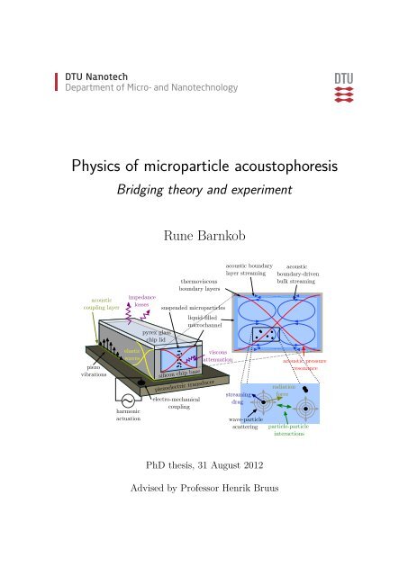
<strong>Physics</strong> <strong>of</strong> <strong>microparticle</strong> <strong>acoustophoresis</strong><br />
<strong>Bridging</strong> <strong>theory</strong> <strong>and</strong> experiment<br />
Rune Barnkob<br />
PhD thesis, 31 August 2012<br />
Advised by Pr<strong>of</strong>essor Henrik Bruus
Cover illustration: Illustration <strong>of</strong> <strong>microparticle</strong> <strong>acoustophoresis</strong> <strong>and</strong> its many physical<br />
aspects.<br />
<strong>Physics</strong> <strong>of</strong> <strong>microparticle</strong> <strong>acoustophoresis</strong> — <strong>Bridging</strong> <strong>theory</strong> <strong>and</strong> experiment<br />
Copyright © 2012 Rune Barnkob All Rights Reserved<br />
Typeset using L A TEX <strong>and</strong> Matlab<br />
http://www.nanotech.dtu.dk/micr<strong>of</strong>luidics<br />
http://rune.barnkob.com<br />
Til min mor,<br />
som gav mig øjne og øre
Abstract<br />
This thesis presents studies <strong>of</strong> <strong>microparticle</strong> <strong>acoustophoresis</strong>, a technique for manipulation<br />
<strong>of</strong> particles in microsystems by means <strong>of</strong> acoustic radiation <strong>and</strong> streaming<br />
forces induced by ultrasound st<strong>and</strong>ing waves. The motivation for the studies<br />
is to increase the theoretical underst<strong>and</strong>ing <strong>of</strong> <strong>microparticle</strong> <strong>acoustophoresis</strong> <strong>and</strong><br />
to develop methods for future advancement <strong>of</strong> its use.<br />
Throughout the work on this thesis the author <strong>and</strong> co-workers 1 have studied<br />
the physics <strong>of</strong> <strong>microparticle</strong> <strong>acoustophoresis</strong> by comparing quantitative measurements<br />
to a theoretical framework consisting <strong>of</strong> existing hydrodynamic <strong>and</strong><br />
acoustic predictions. The theoretical framework is used to develop methods for<br />
in situ determination <strong>of</strong> acoustic energy density <strong>and</strong> acoustic properties <strong>of</strong> <strong>microparticle</strong>s<br />
as well as to design a microchip for high-throughput <strong>microparticle</strong><br />
<strong>acoustophoresis</strong>.<br />
An experimental model system is presented. This system is the center for<br />
the theoretical framework, <strong>and</strong> its underlying assumptions, <strong>of</strong> the acoustophoretic<br />
<strong>microparticle</strong> motion in a suspending liquid subject to harmonic ultrasound<br />
actuation <strong>of</strong> the surrounding microchannel.<br />
Based directly on the governing equations a numerical scheme is set up to<br />
study the transient acoustophoretic motion <strong>of</strong> the <strong>microparticle</strong>s driven by the<br />
acoustic radiation force from sound scattered <strong>of</strong> the particles <strong>and</strong> the Stokes drag<br />
force from the induced acoustic streaming. The numerical scheme is used to<br />
predict the acoustophoretic particle motion in the experimental model system<br />
<strong>and</strong> to study the transition in the motion from being dominated by streaminginduced<br />
drag to being dominated by radiation forces as function <strong>of</strong> particle size,<br />
channel geometry, <strong>and</strong> suspending medium.<br />
Next, is presented an automated <strong>and</strong> temperature-controlled platform for reproducible<br />
<strong>acoustophoresis</strong> measurements suitable for direct comparison to the<br />
theoretical framework. The platform was used to examine in-plane acoustophoretic<br />
particle velocities by micro particle imaging velocimetry. The in-plane particle<br />
velocities are analyzed as function <strong>of</strong> spatial position revealing the complexity <strong>of</strong><br />
the underlying acoustic resonances. The resonances <strong>and</strong> hence the acoustic particle<br />
motion are investigated to determine the dependency on driving voltage,<br />
1 See the list <strong>of</strong> publications, Section 1.3, <strong>and</strong> the introduction to each chapter, Section 1.2.
iv<br />
driving frequency, <strong>and</strong> resonator temperature. Furthermore, the in-plane velocity<br />
measurements form the basis for a systematic investigation <strong>of</strong> the acoustic<br />
radiation- <strong>and</strong> streaming-induced particle velocities as function <strong>of</strong> the particle<br />
size, the actuation frequency, <strong>and</strong> the suspending medium. These measurements<br />
are compared to theoretical predictions showing good agreement.<br />
The acoustophoretic particle motion, <strong>and</strong> in particular the acoustic streaming,<br />
possesses a three-dimensional character. By using the experimental platform<br />
in combination with the Astigmatism micro-PTV technique, preliminary results<br />
are presented <strong>of</strong> the out-<strong>of</strong>-plane acoustophoretic velocities displaying close similarities<br />
to the analytical <strong>and</strong> numerical predictions <strong>of</strong> the theoretical framework.<br />
One <strong>of</strong> the key problems in microchannel <strong>acoustophoresis</strong> is to measure the<br />
absolute size <strong>of</strong> the acoustic energy density, an important parameter when designing<br />
<strong>and</strong> optimizing <strong>acoustophoresis</strong> devices. To facilitate this development, a<br />
number <strong>of</strong> methods are presented to in situ determine the acoustic energy densities<br />
by means <strong>of</strong> acoustophoretic particle motion measured either as particle<br />
trajectories, particle velocities, or particle depletion in terms <strong>of</strong> light-intensity.<br />
Other key parameters when designing <strong>acoustophoresis</strong> devices for particle manipulation<br />
are the acoustic properties, density <strong>and</strong> compressibility <strong>of</strong> the subject<br />
particles. For cells these parameters are widely distributed <strong>and</strong> are seldom known.<br />
For this a method is proposed to in situ determine the density <strong>and</strong> compressibility<br />
<strong>of</strong> a single particle undergoing acoustophoretic motion in an arbitrary acoustic<br />
field.<br />
Finally, the theoretical framework was used as an essential parameter when<br />
designing an <strong>acoustophoresis</strong> microchip allowing for high-throughput particle separation<br />
larger than 1 Liter per hour for a single separation chamber. The design is<br />
based on previously reported design <strong>of</strong> acoustophoretic separators but exp<strong>and</strong>ed<br />
with temperature control allowing for high-power acoustic actuation.
Resumé<br />
Afh<strong>and</strong>lingen <strong>Physics</strong> <strong>of</strong> <strong>microparticle</strong> <strong>acoustophoresis</strong> – <strong>Bridging</strong> <strong>theory</strong> <strong>and</strong> experiment,<br />
Fysikken bag mikropartikel-akust<strong>of</strong>orese – sammenkobling af teori og<br />
eksperiment, er et studie af mikropartikel-akust<strong>of</strong>orese. Mikropartikel-akust<strong>of</strong>orese<br />
er en teknik til manipulering af partikler og væsker i mikrosystemer ved hjælp<br />
af akustiske strålings- og strømningskræfter induceret af stående ultralydsbølger.<br />
Motivationen for dette studie har været at øge den, ind til dato, begrænsede teoretiske<br />
forståelse indenfor mikropartikel-akust<strong>of</strong>orese, samt at udvikle metoder<br />
til fremtidig forbedring inden for dette område.<br />
Gennem ph.d.-projektet har forfatteren og dennes samarbejdspartnere 2 studeret<br />
tidligere beskrivelser af mikropartikel-akust<strong>of</strong>orese. På baggrund af disse<br />
teoretiske forudsigelser – numeriske såvel som analytiske – har vi foretaget kvantitative<br />
målinger med det formål at validere og forbedre de eksisterende forudsigelser<br />
på feltet. Derudover anvendes de eksisterende teoretiske forudsigelser til<br />
at udvikle en række metoder til in situ karakterisering af eksperimentelle akust<strong>of</strong>oretiske<br />
opstillinger og i et enkelt tilfælde til at designe et akust<strong>of</strong>oretisk<br />
separationssystem.<br />
Mere konkret præsenteres der i afh<strong>and</strong>lingen et eksperimentelt model system,<br />
hvor der opsættes en teoretisk beskrivelse af mikropartiklernes akust<strong>of</strong>oretiske<br />
hastighed i en væskefyldt mikrokanal med stående ultralydsbølger. Baseret på de<br />
styrende ligninger beskrives en numerisk model til studie af den akust<strong>of</strong>oretiske<br />
bevægelse af mikropartikler induceret af den akustiske strålingskraft, samt viskøst<br />
træk fra den akustiske strømning. Den numeriske model bruges til at beskrive<br />
overgangen i partiklernes akust<strong>of</strong>oretiske bevægelse fra at være domineret af det<br />
akustiske strømningstræk til at blive domineret af den akustiske strålingskræft.<br />
Denne overgang studeres som funktion af partikelstørrelse, kanalgeometri og den<br />
omgivende væske.<br />
Hernæst præsenteres en automatiseret og temperaturstyret opstilling til reproducerbare<br />
akust<strong>of</strong>orese-målinger, hvilket er velegnet til sammenligning med de<br />
teoretiske forudsigelser. I kombination med mikro-PIV teknikken bruges opstillingen<br />
til at undersøge de akust<strong>of</strong>oretiske plane partikelhastigheder. Disse partikelhastigheder<br />
udersøges som funktion af position i kanalen som afslører den rumlige<br />
2 See publikationslisten, afsnit 1.3, samt introduktionen til de enkelte kapitler, afsnit 1.2.
vi<br />
kompleksitet af de underliggende akustiske resonanser. Ydermere undersøges det<br />
hvordan den påtrykte resonans, og dermed de akustiske partikelbevægelser, responderer<br />
som funktion af den påtrykte drivspænding, frekvens og temperatur.<br />
Endvidere bruges denne type hastighedsmålinger i en systematisk undersøgelse<br />
af de inducerede partikelhastigheder, fra at være domineret af den akustiske<br />
strålingskraft til at være domineret af den akustiske strømning, som funktion af<br />
partikelstørrelse, resonansfrekvens og egenskaberne af den omgivende væske.<br />
Den akust<strong>of</strong>oretiske partikelbevægelse har en tredimensional karakter, især<br />
den akustiske strømning, og ved at bruge den eksperimentelle platform i kombination<br />
med Astigmatisk mikro-PTV teknikken, præsenteres der foreløbige resultater<br />
af de tre-dimensionelle akust<strong>of</strong>oretiske partikelhastigheder som udviser<br />
lighed med de præsenterede analytiske og numeriske forudsigelser.<br />
Et af de centrale problemer i mikropartikel-akust<strong>of</strong>orese er at måle den absolutte<br />
størrelse på den akustiske energitæthed. Dette er en essentiel parameter<br />
ved optimering og design af akust<strong>of</strong>oretiske anvendelser. For at lette denne udvikling,<br />
præsenteres der i afh<strong>and</strong>lingen en række metoder til in situ bestemmelse<br />
af den akustiske energitæthed ved udelukkende at studere akust<strong>of</strong>oretisk partikelbevægelse,<br />
enten målt som partikelbaner, partikelhastigheder eller partiklers<br />
skyggevirkning.<br />
Andre vigtige parametre, når man skal designe akust<strong>of</strong>oretisk udstyr til partikelmanipulation,<br />
er de akustiske egenskaber, densitet og kompressibilitet, af de<br />
manipulerede partikler, fx celler, for hvilke disse parametre sjældent er kendt. I<br />
afh<strong>and</strong>lingen foreslås der en metode til bestemmelse af densitet og kompressibilitet<br />
af en enkelt partikel, som undergår akust<strong>of</strong>oretisk bevægelse i et vilkårligt<br />
akustisk felt. Der præsenteres de næste nødvendige skridt for at realisere denne<br />
metode.<br />
Endelig bruger vi den teoretiske indsigt til at designe en akust<strong>of</strong>orese-mikrochip,<br />
som tillader separationshastigheder på over 1 Liter i timen. Mikrochippens udformning<br />
er baseret på tidligere forskningsresultater, men ved at bruge en temperaturstyring<br />
til sikring af stabile akustiske resonanser, har vi kunnet benytte<br />
høj akustisk aktueringsspænding.
Preface<br />
This thesis is submitted as partial fulfillment for obtaining the degree <strong>of</strong> Doctor<br />
<strong>of</strong> Philosophy (PhD) at the Technical University <strong>of</strong> Denmark (DTU). The PhD<br />
project was financed by the Danish Council for Independent Research, Technology<br />
<strong>and</strong> Production Sciences, Grant No. 274-09-0342. The project was carried out<br />
at the Department <strong>of</strong> Micro- <strong>and</strong> Nanotechnology, DTU Nanotech, as a member<br />
<strong>of</strong> the Theoretical Micr<strong>of</strong>luidics Group (TMF) during a three-year period from<br />
September 2009 to August 2012. The project was supervised by Pr<strong>of</strong>essor Henrik<br />
Bruus, leader <strong>of</strong> the TMF group at DTU Nanotech. During many short visits<br />
throughout all three project years <strong>and</strong> in the period from September to November<br />
2010 I worked in the lab <strong>of</strong> Pr<strong>of</strong>essor Thomas Laurell at Lund University,<br />
Sweden. During the period from February to July 2010, I visited the University<br />
<strong>of</strong> California, Santa Barbara, CA, USA, together with the rest <strong>of</strong> the TMF group<br />
<strong>and</strong> I worked with the group <strong>of</strong> Pr<strong>of</strong>essor Tom Soh, <strong>and</strong> in August 2010 I visited<br />
the group <strong>of</strong> Pr<strong>of</strong>essor Steve Wereley for a week at Purdue University, IN, USA.<br />
Lastly, in the period from November to December 2010 I worked in the lab <strong>of</strong><br />
Martin Wiklund, Royal Institute <strong>of</strong> Technology, Stockholm, Sweden.<br />
As evident from the many above-mentioned visits to experimental research<br />
groups this thesis is the outcome <strong>of</strong> fruitful collaborations with many smart people,<br />
whom I will like to acknowledge. Primarily <strong>and</strong> firstly, I will like to thank<br />
Pr<strong>of</strong>essor Henrik Bruus for always being there to make sure that I grew up as<br />
a scientist with no compromises when it comes to scientific detail <strong>and</strong> accuracy.<br />
Henrik has been a superb supervisor <strong>and</strong> mentor as well as a good friend. We<br />
have had many great times academically as well as less academically ranging from<br />
altitude, latitude, <strong>and</strong> longitude bets in the Ecuadorian jungle to lots <strong>of</strong> visits to<br />
cafés around the world <strong>and</strong> in particular in Copenhagen.<br />
Next, I will like to thank Thomas Laurell <strong>and</strong> the rest <strong>of</strong> Elmät for always<br />
keeping a door open for me. In particular, I will like to thank Per Augustsson for<br />
a fruitful collaboration, academically as well as personally <strong>and</strong> for always being<br />
(too) skeptical — I cross my fingers that our collaboration continues somehow.<br />
Thanks to Martin Wiklund for good discussions <strong>and</strong> for inviting me to the capital<br />
<strong>of</strong> Sc<strong>and</strong>inavia, <strong>and</strong> Ida Iranmanesh for good collaboration <strong>and</strong> Fesenjun. Thanks<br />
to Tom Soh for hosting me in sunny California, Lore Dobler for flowers, <strong>and</strong> the
viii<br />
rest <strong>of</strong> the Soh <strong>and</strong> Pennathur groups for margaritas <strong>and</strong> BBQ. Thanks to Steve<br />
Wereley for PIV <strong>and</strong> EDPIV, <strong>and</strong> a nice stay in Indiana. Thanks to Christian<br />
Kähler <strong>and</strong> his group, in particular Álvaro Marín <strong>and</strong> Massimiliano Rossi for<br />
great <strong>and</strong> joyful co-working. Thanks to Mads Jakob H. Jensen for COMSOL<br />
tricks <strong>and</strong> thanks to all the TMF members that I passed during the 4 years, <strong>and</strong><br />
in particular Peter Barkholt Muller for being the best acoustic buddy ever <strong>and</strong><br />
Mathias Bækbo Andersen for being a tremendous study buddy throughout nine<br />
years at DTU <strong>and</strong> about. Thanks to all my friends <strong>and</strong> family, you know who<br />
you are <strong>and</strong> your support through this project is highly appreciated.<br />
Kongens Lyngby, 31 August 2012<br />
Rune Barnkob
Contents<br />
Preliminaries<br />
i<br />
Abstract . . . . . . . . . . . . . . . . . . . . . . . . . . . . . . . . . . . iii<br />
Resumé . . . . . . . . . . . . . . . . . . . . . . . . . . . . . . . . . . . v<br />
Preface . . . . . . . . . . . . . . . . . . . . . . . . . . . . . . . . . . . . vii<br />
Contents . . . . . . . . . . . . . . . . . . . . . . . . . . . . . . . . . . . x<br />
List <strong>of</strong> Figures . . . . . . . . . . . . . . . . . . . . . . . . . . . . . . . . xii<br />
List <strong>of</strong> Tables . . . . . . . . . . . . . . . . . . . . . . . . . . . . . . . . xiii<br />
List <strong>of</strong> Symbols <strong>and</strong> Acronyms . . . . . . . . . . . . . . . . . . . . . . . xiv<br />
List <strong>of</strong> Material Parameters . . . . . . . . . . . . . . . . . . . . . . . . xvi<br />
1 Introduction 1<br />
1.1 Length scales <strong>and</strong> frequencies . . . . . . . . . . . . . . . . . . . . 2<br />
1.2 Thesis outline . . . . . . . . . . . . . . . . . . . . . . . . . . . . . 2<br />
1.3 Publications during the PhD studies . . . . . . . . . . . . . . . . 5<br />
2 <strong>Physics</strong> <strong>of</strong> <strong>acoustophoresis</strong> 9<br />
2.1 Experimental model system . . . . . . . . . . . . . . . . . . . . . 9<br />
2.2 Acoustic actuation . . . . . . . . . . . . . . . . . . . . . . . . . . 11<br />
2.3 Concluding remarks . . . . . . . . . . . . . . . . . . . . . . . . . . 17<br />
3 Theory <strong>of</strong> <strong>acoustophoresis</strong> 19<br />
3.1 Governing equations <strong>of</strong> a thermoviscous fluid . . . . . . . . . . . . 19<br />
3.2 Resonances . . . . . . . . . . . . . . . . . . . . . . . . . . . . . . 24<br />
3.3 Acoustic radiation force on a <strong>microparticle</strong> . . . . . . . . . . . . . 26<br />
3.4 Boundary-induced acoustic streaming . . . . . . . . . . . . . . . . 28<br />
3.5 Acoustophoretic single-particle velocities . . . . . . . . . . . . . . 31<br />
3.6 Concluding remarks . . . . . . . . . . . . . . . . . . . . . . . . . . 35<br />
4 Numerics <strong>of</strong> <strong>acoustophoresis</strong> 37<br />
4.1 Numerical model . . . . . . . . . . . . . . . . . . . . . . . . . . . 37<br />
4.2 Numerical results . . . . . . . . . . . . . . . . . . . . . . . . . . . 41<br />
4.3 Concluding remarks . . . . . . . . . . . . . . . . . . . . . . . . . 49
x<br />
CONTENTS<br />
5 Acoustophoresis analyzed by micro-PIV 51<br />
5.1 Automated <strong>and</strong> temperature-controlled <strong>acoustophoresis</strong> platform . 52<br />
5.2 µPIV for <strong>acoustophoresis</strong> measurements . . . . . . . . . . . . . . . 55<br />
5.3 Global resonance structure . . . . . . . . . . . . . . . . . . . . . . 63<br />
5.4 Frequency, voltage, <strong>and</strong> temperature . . . . . . . . . . . . . . . . 64<br />
5.5 Determination <strong>of</strong> the radiation-to-streaming transition . . . . . . 67<br />
5.6 Concluding remarks . . . . . . . . . . . . . . . . . . . . . . . . . . 75<br />
6 Acoustophoresis analyzed by Astigmatism micro-PTV 77<br />
6.1 A short intro to Astigmatism µPTV . . . . . . . . . . . . . . . . . 78<br />
6.2 Experimental setup . . . . . . . . . . . . . . . . . . . . . . . . . . 79<br />
6.3 Acoustophoresis measurements by Astigmatism µPTV . . . . . . 79<br />
6.4 Concluding remarks . . . . . . . . . . . . . . . . . . . . . . . . . . 82<br />
7 Applications <strong>of</strong> <strong>acoustophoresis</strong> 85<br />
7.1 Determination in situ <strong>of</strong> acoustic energy densities . . . . . . . . . 85<br />
7.2 Determination <strong>of</strong> density <strong>and</strong> compressibility <strong>of</strong> <strong>microparticle</strong>s using<br />
microchannel <strong>acoustophoresis</strong> . . . . . . . . . . . . . . . . . . 104<br />
7.3 High-throughput cell separation using high-voltage temperaturecontrolled<br />
<strong>acoustophoresis</strong> . . . . . . . . . . . . . . . . . . . . . . 106<br />
8 Conclusion <strong>and</strong> outlook 109<br />
A Paper published in Lab on a Chip, January 2010 113<br />
B Paper published in Lab on a Chip, October 2011 123<br />
C Paper published in Lab on a Chip, March 2012 139<br />
D Paper published in J Micromech Microeng, June 2012 149<br />
E Paper published in Lab on a Chip, July 2012 159<br />
F Paper published in Phys Rev E, November 2012 171<br />
Bibliography 189
List <strong>of</strong> Figures<br />
1.1 Overview <strong>of</strong> length scales treated in this thesis. . . . . . . . . . . 2<br />
1.2 Overview <strong>of</strong> frequencies treated in this thesis. . . . . . . . . . . . 3<br />
2.1 Experimental <strong>acoustophoresis</strong> model system. . . . . . . . . . . . . 10<br />
2.2 Acoustic actuation <strong>of</strong> the experimental model system. . . . . . . . 13<br />
3.1 Acoustic eigenmode in a liquid rectangular cuboid. . . . . . . . . 25<br />
3.2 Rayleigh’s classical result for the parallel-plate streaming. . . . . . 29<br />
3.3 Ratio <strong>of</strong> radiation- <strong>and</strong> streaming-induced particle velocities. . . . 32<br />
3.4 Transverse particle path for radiation-dominated <strong>acoustophoresis</strong>. 34<br />
4.1 Mesh convergence analysis <strong>of</strong> numerical <strong>acoustophoresis</strong> model. . . 40<br />
4.2 Numerical modeling <strong>of</strong> the ultrasound actuation. . . . . . . . . . . 41<br />
4.3 Numerical modeling <strong>of</strong> the first-order acoustic fields in the bulk fluid. 42<br />
4.4 Numerical modeling <strong>of</strong> the first-order fields near boundaries. . . . 43<br />
4.5 Numerical modeling <strong>of</strong> the second-order acoustic fields. . . . . . . 44<br />
4.6 Numerical modeling <strong>of</strong> acoustophoretic particle tracks. . . . . . . 46<br />
4.7 Numerical modeling <strong>of</strong> <strong>acoustophoresis</strong> in a high channel. . . . . . 47<br />
4.8 Numerical modeling <strong>of</strong> <strong>acoustophoresis</strong> in high-viscosity medium. 49<br />
5.1 Automated <strong>and</strong> temperature-controlled <strong>acoustophoresis</strong> platform. 53<br />
5.2 µPIV image frame <strong>and</strong> particle velocity example. . . . . . . . . . 55<br />
5.3 µPIV image-pair time shift <strong>and</strong> st<strong>and</strong>ard deviation. . . . . . . . . 59<br />
5.4 µPIV interrogation window size <strong>and</strong> repeated measurements. . . . 60<br />
5.5 µPIV measurement <strong>of</strong> the spatial <strong>acoustophoresis</strong> structure. . . . 62<br />
5.6 Acoustophoretic velocity magnitude along the channel. . . . . . . 63<br />
5.7 Acoustophoretic velocity as function <strong>of</strong> frequency <strong>and</strong> temperature. 66<br />
5.8 1-µm acoustophoretic particle velocities. . . . . . . . . . . . . . . 70<br />
5.9 Transverse acoustophoretic velocities. . . . . . . . . . . . . . . . . 71<br />
5.10 Acoustophoretic velocity amplitudes versus particle diameter. . . . 72<br />
5.11 Collapsing acoustophoretic velocity data by theoretical prediction. 74<br />
6.1 Working principle <strong>of</strong> the Astigmatism µPTV technique. . . . . . . 78
xii<br />
List <strong>of</strong> Figure<br />
6.2 A-µPTV measurements <strong>of</strong> radiation-dominated <strong>acoustophoresis</strong>. . 80<br />
6.3 A-µPTV measurements <strong>of</strong> streaming-dominated <strong>acoustophoresis</strong>. . 81<br />
6.4 A-µPTV experiments <strong>and</strong> analytical streaming prediction. . . . . 82<br />
6.5 Comparing A-µPTV result to analytical streaming prediction. . . 82<br />
7.1 Setup used to test E ac -determination by particle tracking. . . . . 87<br />
7.2 Acoustic energy density measured from particle track. . . . . . . . 88<br />
7.3 Acoustic energy density as versus piezo driving voltage. . . . . . . 89<br />
7.4 Acoustic energy density as function <strong>of</strong> piezo driving frequency. . . 90<br />
7.5 Simplified 2D modeling <strong>of</strong> resonances in chip <strong>and</strong> channel. . . . . 92<br />
7.6 Acoustic energy density measured from particle velocity pr<strong>of</strong>ile. . 93<br />
7.7 Experimental channel used for testing light-intensity method. . . . 94<br />
7.8 Sketch <strong>of</strong> the light-intensity model. . . . . . . . . . . . . . . . . . 97<br />
7.9 Experimental setup used to test the light-intensity method. . . . . 98<br />
7.10 Examining images used to test the light-intensity method. . . . . 100<br />
7.11 Acoustic energy densities using the light-intensity method. . . . . 102
List <strong>of</strong> Tables<br />
2.1 Dimensions <strong>of</strong> the experimental model system . . . . . . . . . . . 11<br />
2.2 Primary theoretical assumptions used throughout the thesis. . . . 12<br />
3.1 Wall drag-correction factors χ for particle sizes treated in the thesis. 35<br />
5.1 Depth <strong>of</strong> correlation for range <strong>of</strong> particle diameters . . . . . . . . 57<br />
5.2 Nominal <strong>and</strong> the measured particle diameters. . . . . . . . . . . . 67<br />
5.3 Results <strong>of</strong> the measured streaming coefficients. . . . . . . . . . . 73<br />
5.4 Measured relative particle velocities for different particle sizes. . . 75
xiv<br />
List <strong>of</strong> Symbols<br />
List <strong>of</strong> Symbols <strong>and</strong> Acronyms<br />
Symbol Description Unit<br />
a Microparticle radius m<br />
BAW<br />
Bulk Acoustic Wave<br />
c Isentropic speed <strong>of</strong> sound m s −1<br />
C Particle concentration m −3<br />
C (g)<br />
Relative convergence parameter<br />
C corr<br />
PIV cross-correlation function<br />
C p Specific heat capacity, constant pressure J kg −1 K −1<br />
C v Specific heat capacity, constant volume J kg −1 K −1<br />
D th ≡ k th<br />
ρC p<br />
Thermal diffusivity m 2 s −1<br />
E ac Time-average acoustic energy density J m −3<br />
f Frequency s −1<br />
f 1<br />
Compressibility factor in F rad<br />
f 2 Density factor in F rad .<br />
F drag Viscous Stokes drag force N<br />
F rad Acoustic radiation force N<br />
i<br />
Unit imaginary number<br />
K = κ −1 Bulk modulus Pa<br />
k = 2π = f Acoustic wavenumber m −1<br />
λ c<br />
k th Thermal conductivity W m −1 K −1<br />
l, w, h Microchannel length, width, <strong>and</strong> height m<br />
n<br />
Outward-pointing normal vector<br />
p Pressure Pa<br />
piezo (or PZT) Piezoelectric transducer<br />
PID<br />
Proportional–Integral–Derivative controller<br />
PIV<br />
Particle Image Velocimetry<br />
PTV<br />
Particle Tracking Velocimetry<br />
PZT<br />
Lead Zirconate Titanate<br />
s Entropy per unit mass J K −1 kg −1<br />
S PIV interrogation window side length pixels<br />
SAW<br />
Surface Acoustic Wave<br />
t Time s<br />
T Temperature K<br />
u Acoustophoretic particle velocity m s −1<br />
U pp Piezo peak-to-peak voltage V<br />
v Fluid velocity vector m s −1<br />
v Fluid velocity magnitude m s −1<br />
〈v 2 〉 Steady acoustic streaming velocity m s −1<br />
V Volume m 3
List <strong>of</strong> Symbols <strong>and</strong> Acronyms<br />
xv<br />
Symbol Description Unit<br />
α Isobaric thermal expansion K −1<br />
β = 1/3<br />
Viscosity ratio<br />
δ Viscous boundary layer thickness m<br />
˜δ = δ/a<br />
Normalized viscous boundary layer thickness<br />
δ th Thermal boundary layer thickness m<br />
δ ij<br />
Kronecker’s delta<br />
ɛ Internal energy per unit mass J kg −1<br />
η Dynamic viscosity Pa s<br />
γ = C p /C v Specific heat ratio<br />
γ att<br />
Viscous attenuation factor<br />
Γ<br />
Viscous correction factor to F rad<br />
κ = K −1 Isothermal compressibility Pa −1<br />
˜κ = κ p /κ 0 Compressibility ratio for particle <strong>and</strong> liquid<br />
λ Acoustic wavelength m<br />
ν Kinematic viscosity (momentum diffusivity) m 2 s −1<br />
ω = 2πf Angular frequency s −1<br />
Ω<br />
Domain<br />
∂Ω<br />
Domain boundary<br />
Φ<br />
Acoustic contrast factor in F rad<br />
ρ Mass density kg m −3<br />
˜ρ = ρ p /ρ 0 Mass density ratio for particle <strong>and</strong> liquid<br />
σ ′ Viscous stress tensor Pa<br />
ζ Second coefficient <strong>of</strong> viscosity Pa s<br />
¯□<br />
Complex conjugate <strong>of</strong> the function □<br />
□ i<br />
i’th component <strong>of</strong> the function □, i = x, y, z<br />
□ 0 , □ 1 , □ 2 1st-, 2nd-, <strong>and</strong> 3rd-order perturbations <strong>of</strong> □<br />
□ a<br />
Amplitude <strong>of</strong> the first-order field □<br />
´<br />
〈□〉 = 1 t+τ<br />
□ dt, Time average <strong>of</strong> function □<br />
τ t<br />
〈□〉 △<br />
Average <strong>of</strong> function □ taken over △<br />
∂ □<br />
Partial derivative with respect to □<br />
(x, y, z) Cartesian coordinates m
xvi<br />
List <strong>of</strong> Symbols<br />
List <strong>of</strong> Material Parameters<br />
All material parameters are listed at 25 ◦ C unless otherwise stated.<br />
Polystyrene<br />
Density ρ p 1050 kg m −3 Ref. [1]<br />
Speed <strong>of</strong> sound (at 20 ◦ C) c p 2350 m s −1 Ref. [2]<br />
Poisson’s ratio σ p 0.35 Ref. [3]<br />
Compressibility κ p 249 TPa −1 See a.<br />
Polyamide<br />
Density ρ p 1030 kg m −3 See d.<br />
Speed <strong>of</strong> sound (for Nylon) c p 2660 m s −1 Ref. [1]<br />
Compressibility κ p 137 TPa −1 See b.<br />
Water<br />
Density ρ 0 997 kg m −3 Ref. [1]<br />
Speed <strong>of</strong> sound c 0 1497 m s −1 Ref. [1]<br />
Charact. acoustic impedance Z 0 1.49 ×10 6 kg m −2 s −1 Z 0 = ρ 0 c 0<br />
Viscosity η 0.890 mPa s Ref. [1]<br />
Viscous boundary layer, 1.940 MHz δ 0.38 µm Eq. (3.15b)<br />
Viscous boundary layer, 3.900 MHz δ 0.27 µm Eq. (3.15b)<br />
Compressibility κ 0 448 TPa −1 See b.<br />
Compressibility factor (polystyrene) f 1 0.444 Eq. (3.30a)<br />
Density factor (polystyrene) f 2 0.034 Eq. (3.30b)<br />
Contrast factor (polystyrene) Φ 0.165 Eq. (3.33)<br />
Normalized momentum diffusivity ν/Φ 5.25 mm 2 s −1<br />
Thermal conductivity k th 0.603 W m −1 K −1 Ref. [4]<br />
Specific heat capacity C p 4183 J kg −1 K −1 Ref. [4]<br />
Specific heat capacity ratio γ 1.014 Eq. (3.10)<br />
Thermal diffusivity D th 1.43 ×10 −7 m 2 s −1 Eq. (3.13)<br />
Thermal expansion coefficient α 2.97 ×10 −4 K −1 Ref. [1], c.<br />
0.75:0.25 mixture <strong>of</strong> water <strong>and</strong> glycerol<br />
Density ρ 0 1063 kg m −3 Ref. [5]<br />
Speed <strong>of</strong> sound c 0 1611 m s −1 Ref. [6]<br />
Viscosity η 1.787 mPa s Ref. [5]<br />
Viscous boundary layer, 2.027 MHz δ 0.51 µm Eq. (3.15b)<br />
Compressibility κ 0 363 TPa −1 See b.<br />
Compressibility factor (polystyrene) f 1 0.313 Eq. (3.30a)<br />
Density factor (polystyrene) f 2 -0.008 Eq. (3.30b)<br />
Contrast factor (polystyrene) Φ 0.10 Eq. (3.33)<br />
Normalized momentum diffusivity ν/Φ 16.8 mm 2 s −1<br />
0.50:0.50 mixture <strong>of</strong> water <strong>and</strong> glycerol<br />
Density ρ 0 1129 kg m −3 Ref. [5]<br />
Speed <strong>of</strong> sound c 0 1725 m s −1 Ref. [6]<br />
Viscosity η 5.00 mPa s Ref. [5]<br />
Viscous boundary layer, 2.270 MHz δ 0.79 µm Eq. (3.15b)<br />
Compressibility κ 0 298 TPa −1 See b.<br />
Compressibility factor (polystyrene) f 1 0.164 Eq. (3.30a)
List <strong>of</strong> Material Parameters<br />
xvii<br />
Density factor (polystyrene) f 2 -0.049 Eq. (3.30b)<br />
Contrast factor (polystyrene) Φ 0.030 Eq. (3.33)<br />
Normalized momentum diffusivity ν/Φ 146 mm 2 s −1<br />
Thermal conductivity (at 20 ◦ C) k th 0.416 W m −1 K −1 Ref. [7]<br />
Specific heat capacity (at 1.7 ◦ C) C p 3360 J kg −1 K −1 Ref. [8]<br />
Specific heat capacity ratio γ 1.04 Eq. (3.10)<br />
Thermal diffusivity D th 1.10 ×10 −7 m 2 s −1 Eq. (3.13)<br />
Thermal expansion coefficient α 4.03 ×10 −4 K −1 Ref. [1], c.<br />
Air<br />
Density ρ air 1.16 kg m −3 Ref. [1]<br />
Speed <strong>of</strong> sound c air 343.4 m s −1 Ref. [1]<br />
Charact. acoustic impedance Z air 3.99 ×10 5 kg m −2 s −1 Z air = ρ air c air<br />
Pyrex glass<br />
Density ρ py 2230 kg m −3 Ref. [1]<br />
Charact. acoustic impedance Z py 1.25 ×10 7 kg m −2 s −1 Z py = ρ py c py<br />
Young’s modulus Y py 62.6 GPa [4]<br />
Poisson’s ratio σ py 0.225 [4]<br />
Speed <strong>of</strong> sound, longitudinal c py 5640 m s −1 See e.<br />
Silicon<br />
Density ρ si 2331 kg m −3 Ref. [1]<br />
Speed <strong>of</strong> sound, longitudinal c si 8490 m s −1<br />
Charact. acoustic impedance Z si 1.98 ×10 7 kg m −2 s −1 Z si = ρ si c si<br />
a Calculated as κ p = 3(1−σp)<br />
1<br />
1+σ p ρ p c 2 p<br />
from Ref. [9].<br />
b Calculated as κ 0 = 1/ ( ρ 0 c 2 0)<br />
.<br />
c Calculated as α = − (1/ρ) (∂ T ρ) p<br />
.<br />
d ORGASOL1 5 mm: http://r427a.com/technical-polymers/orgasol-powders/ technical-datasheets.<br />
√ e Calculated as c L = 1−σ Y<br />
(1+σ)(1−2σ) ρ<br />
from Ref. [9].
xviii<br />
List <strong>of</strong> Symbols
Chapter 1<br />
Introduction<br />
Manipulation <strong>and</strong> separation <strong>of</strong> particles <strong>and</strong> fluids are used in a broad range <strong>of</strong><br />
research. Especially the manipulation, separation, purification, <strong>and</strong> isolation <strong>of</strong><br />
bioparticles <strong>and</strong> cells in complex bi<strong>of</strong>luids are becoming essential within the areas<br />
<strong>of</strong> biology <strong>and</strong> medicine. For this, the technology <strong>of</strong> lab-on-a-chip <strong>and</strong> micr<strong>of</strong>luidics<br />
provides a large potential for creating high performance manipulation <strong>and</strong><br />
separation applications due to precise <strong>and</strong> accurate control <strong>of</strong> the forces driving<br />
the manipulation [10–12]. Typically, such forces are hydrodynamic, electric, dielectric,<br />
magnetic, <strong>and</strong> mechanical contact forces. Acoustic forces are also being<br />
used for the manipulation <strong>of</strong> fluids <strong>and</strong> suspended particles, where the migration<br />
due to sound are <strong>of</strong>ten termed <strong>acoustophoresis</strong>.<br />
The ability to use acoustic forces for manipulation <strong>of</strong> particles <strong>and</strong> fluids are<br />
well-known <strong>and</strong> has a long history dating back to scientists including Chladni,<br />
Savart, Faraday, Kundt, <strong>and</strong> Rayleigh. It is thus a classical field that has now<br />
found new life in the modern research in the form <strong>of</strong> acoust<strong>of</strong>luidics, the use <strong>of</strong><br />
ultrasound acoustic fields for application in micr<strong>of</strong>luidics. The acoust<strong>of</strong>luidics<br />
research field has received increasing interest since the early 90s by work <strong>of</strong> M<strong>and</strong>ralis<br />
<strong>and</strong> Feke [13, 14], Yasuda et al. [15], Johnson <strong>and</strong> Feke [16], <strong>and</strong> Hawkes<br />
<strong>and</strong> Coakley [17] 1 . Excellent acoust<strong>of</strong>luidics reviews are given by Friend <strong>and</strong> Yeo<br />
in Review in Modern <strong>Physics</strong> with the emphasis on surface acoustic wave devices<br />
[19] <strong>and</strong> in the on-going 23-articles-long tutorial series in Lab on a Chip focusing<br />
on bulk acoustic wave devices [20].<br />
The research field <strong>of</strong> acoust<strong>of</strong>luidics is now exp<strong>and</strong>ing rapidly as scientists realize<br />
its high potential for gentle, label-free, <strong>and</strong> purely mechanical manipulation<br />
<strong>of</strong> particles <strong>and</strong> fluids. During the last decade acoust<strong>of</strong>luidics has been applied to<br />
numerous useful purposes, such as medium exchange <strong>of</strong> yeast cells [21], separation<br />
<strong>of</strong> lipids from blood cells [22], phage display selection [23], selective bioparticle<br />
retention [24], raw milk control [25], whole-blood plasmapheresis [26], forensic<br />
1 An excellent historic review are given in the PhD thesis <strong>of</strong> Per Augustsson [18].
2 Introduction<br />
homo sapiens<br />
mosquito<br />
width <strong>of</strong><br />
human hair<br />
bacteria<br />
virus<br />
width <strong>of</strong> DNA<br />
water<br />
molecule<br />
microchip width<br />
<strong>microparticle</strong>s<br />
microchannel width<br />
Figure 1.1: Length scales treated in this thesis (blue) in context to other length scales.<br />
The lengths are all approximate <strong>and</strong> are inspired by numerous sources on Wikipedia.<br />
analysis <strong>of</strong> sexual assault evidence [27], cell cycle synchronization <strong>of</strong> mammalian<br />
cells [28], enrichment <strong>of</strong> prostate cancer cells from blood [29], study <strong>of</strong> natural<br />
killer cells [30], single-cell manipulation [31], <strong>and</strong> trapping <strong>of</strong> bacteria [32]. In<br />
addition, <strong>acoustophoresis</strong> is being used commercially for the acoustic focusing<br />
cytometer from Life Technologies.<br />
However, for future development, the research <strong>of</strong> acoust<strong>of</strong>luidics faces crucial<br />
challenges, including the increase <strong>of</strong> separation <strong>and</strong> manipulation throughput,<br />
the ability to h<strong>and</strong>le suspensions <strong>of</strong> physiological relevant concentrations, <strong>and</strong> the<br />
separation <strong>and</strong> manipulation <strong>of</strong> sub-micrometer particles such as small bacteria,<br />
vira, <strong>and</strong> biomolecules.<br />
To date acoust<strong>of</strong>luidics has mainly been driven by applications <strong>of</strong>ten leaving<br />
room for improvements regarding the underst<strong>and</strong>ing <strong>of</strong> the underlying physical<br />
phenomena. Hence, the motivation for this thesis is to increase the theoretical<br />
underst<strong>and</strong>ing <strong>of</strong> <strong>microparticle</strong> <strong>acoustophoresis</strong>. To do this we carry out theoretical<br />
<strong>and</strong> experimental analyses to validate <strong>and</strong> exp<strong>and</strong> existing predictions <strong>and</strong><br />
to develop methods for future enhancement <strong>of</strong> acoust<strong>of</strong>luidics.<br />
1.1 Length scales <strong>and</strong> frequencies<br />
The thesis involves the science <strong>of</strong> sound (ultrasound) in small mm-sized systems,<br />
<strong>and</strong> in Fig. 1.1 <strong>and</strong> Fig. 1.2 are shown the length scales <strong>and</strong> acoustic frequencies<br />
treated in this work, respectively.<br />
1.2 Thesis outline<br />
This thesis consists <strong>of</strong> 8 chapters, where<strong>of</strong> most <strong>of</strong> the content included is already<br />
published (or sent for publication) in journals <strong>and</strong> conference proceedings as listed<br />
in Section 1.3. The thesis is naturally built around the six journal papers, which<br />
are all enclosed in the appendices Chapters A to F, <strong>and</strong> the thesis constitutes
1.2 Thesis outline 3<br />
Human heartbeat<br />
Severe weather<br />
Earthquake waves<br />
Volcanoes<br />
Ultrasonic cleaners<br />
Whale sounds<br />
Human hearing<br />
Bat sonar<br />
Medical ultrasound<br />
Ultrasound acoust<strong>of</strong>luidics<br />
Surface acoustic waves<br />
in nanostructures<br />
Frequency [Hz]<br />
Figure 1.2: Acoustic frequencies <strong>of</strong> “Ultrasound acoust<strong>of</strong>luidics” (blue) in the context<br />
<strong>of</strong> acoustic frequencies encountered in modern human life. The frequencies are all<br />
approximate <strong>and</strong> are inspired by Ref. [33] <strong>and</strong> various sources on the world wide web.<br />
a combined presentation connecting the various parts <strong>of</strong> the work. Most <strong>of</strong> the<br />
work is part <strong>of</strong> collaborations with colleagues <strong>and</strong> therefore each chapter starts<br />
with a list <strong>of</strong> relevant collaborators.<br />
Here follows as list <strong>of</strong> all the chapter titles <strong>and</strong> brief outlines <strong>of</strong> their content.<br />
Chapter 2 — <strong>Physics</strong> <strong>of</strong> <strong>acoustophoresis</strong>. This chapter provides an introduction<br />
to the physics <strong>of</strong> <strong>microparticle</strong> <strong>acoustophoresis</strong>. We introduce our experimental<br />
model system representing the class <strong>of</strong> hard-material acoustic devices for<br />
generation <strong>of</strong> bulk acoustic resonances driven by an attached piezoelectric transducer.<br />
With the experimental model system in mind, we map the acoustic <strong>and</strong><br />
hydrodynamic effects important for underst<strong>and</strong>ing the acoustophoretic <strong>microparticle</strong><br />
motion, <strong>and</strong> we state the primary assumptions constituting the basis <strong>of</strong> the<br />
theoretical descriptions in this thesis.<br />
Chapter 3 — Theory <strong>of</strong> <strong>acoustophoresis</strong>. We set up the mathematical<br />
framework for this thesis based on the phenomena <strong>and</strong> approximations presented<br />
in Chapter 2. We introduce the governing equations for a thermoviscous fluid<br />
<strong>and</strong> we derive the acoustic wave equation for the isentropic assumption which is<br />
suitable when investigating the underlying eigenmodes <strong>of</strong> the acoustic resonator.<br />
We further describe the time-averaged second-order phenomena <strong>of</strong> the acoustic<br />
radiation force acting on suspended particles as well as the boundary-induced<br />
acoustic streaming flow. Finally, we set up the equation <strong>of</strong> motion for suspended<br />
<strong>microparticle</strong>s as they undergo <strong>acoustophoresis</strong>.<br />
Chapter 4 — Numerics <strong>of</strong> <strong>acoustophoresis</strong>. We set up a numerical model<br />
for the <strong>microparticle</strong> <strong>acoustophoresis</strong> in the experimental model system presented<br />
in Chapter 2. The model is based directly on the governing equations presented<br />
in Chapter 3 implemented <strong>and</strong> solved using the commercial finite element s<strong>of</strong>tware<br />
COMSOL Multiphysics. Using the model we show the transition in the
4 Introduction<br />
<strong>microparticle</strong> <strong>acoustophoresis</strong> from being dominated by the streaming-induced<br />
drag forces to being dominated by the acoustic radiation forces. Furthermore we<br />
demonstrate how this transition depends on particle size, channel geometry, <strong>and</strong><br />
suspending medium. This chapter is based on the journal paper appended in<br />
Chapter E.<br />
Chapter 5 — Acoustophoresis analyzed by micro-PIV. We present an<br />
automated <strong>and</strong> temperature-controlled experimental platform for analyzing the<br />
experimental model system in a stable <strong>and</strong> reproducible manner. The platform<br />
was used to carry out micro-PIV measurements <strong>of</strong> the in-plane acoustophoretic<br />
<strong>microparticle</strong> motion. The measurements were carried out for a large fraction<br />
<strong>of</strong> the investigated microchannel providing insight in the complexity <strong>of</strong> the<br />
acoustophoretic motion. Moreover, the actuation frequency <strong>and</strong> temperature are<br />
scanned in order to investigate the peak widths <strong>and</strong> temperature sensitivities <strong>of</strong><br />
the underlying acoustic resonances. Finally, we use the micro-PIV setup to investigate<br />
the interplay between the radiation- <strong>and</strong> streaming-induced forces on<br />
<strong>microparticle</strong>s. We verify a theoretical prediction <strong>of</strong> the ratio <strong>of</strong> the radiation<strong>and</strong><br />
streaming-induced particle velocities <strong>and</strong> we demonstrate control over this<br />
ratio by adjusting the particle size, the actuation frequency, <strong>and</strong> the suspending<br />
medium. This chapter is based on the journal papers appended in Chapters B<br />
<strong>and</strong> F.<br />
Chapter 6 — Acoustophoresis analyzed by Astigmatism micro-PTV.<br />
In order to measure the out-<strong>of</strong>-plane velocity components <strong>of</strong> the acoustophoretic<br />
<strong>microparticle</strong> motion, we extend the automated <strong>and</strong> temperature-controlled<br />
<strong>acoustophoresis</strong> platform presented in Chapter 5 for use in combination with the<br />
Astigmatism micro-PTV technique. We show the transition in the acoustophoretic<br />
particle motion from being dominated by the streaming-induced drag for small<br />
particles to being dominated by the radiation forces for larger particles. From the<br />
motion <strong>of</strong> the smallest particles we compare the measured acoustic streaming to<br />
analytical predictions. This chapter is based on preliminary work to be presented<br />
at the “µFlu2012” conference [34].<br />
Chapter 7 — Applications <strong>of</strong> <strong>acoustophoresis</strong>. We present three applications<br />
<strong>of</strong> <strong>microparticle</strong> <strong>acoustophoresis</strong>: (i) In order to improve the development<br />
<strong>and</strong> optimization <strong>of</strong> <strong>acoustophoresis</strong> microdevices we propose a set <strong>of</strong> methods for<br />
in situ determination <strong>of</strong> the acoustic energy density. All methods are based on the<br />
assumption <strong>of</strong> a locally well-known transverse resonance but they rely on different<br />
measurement probes such as particle trajectories, particle velocities, <strong>and</strong> light<br />
intensities. (ii) Using a theoretical expression for the acoustic radiation force <strong>and</strong><br />
the measurements <strong>of</strong> acoustophoretic particle motion as presented in Chapter 5<br />
<strong>and</strong> 6 we propose a method for determination <strong>of</strong> the density <strong>and</strong> compressibility<br />
<strong>of</strong> individual <strong>microparticle</strong>s. (iii) We present a high-throughput <strong>acoustophoresis</strong><br />
chip based on maintaining a stable resonance by use <strong>of</strong> temperature control allowing<br />
for large actuation voltages enabling high-throughput separation <strong>of</strong> cells
1.3 Publications during the PhD studies 5<br />
in suspension. This chapter is based on the journal papers appended in Chapters<br />
A, C, <strong>and</strong> D.<br />
Chapter 8 — Conclusions <strong>and</strong> outlook. We end the thesis with a summation<br />
<strong>of</strong> our findings <strong>and</strong> give an outlook for further suitable routes <strong>of</strong> physics studies<br />
<strong>of</strong> <strong>microparticle</strong> <strong>acoustophoresis</strong> to advance the development <strong>of</strong> the acoust<strong>of</strong>luidics<br />
research field.<br />
1.3 Publications during the PhD studies<br />
During my PhD studies I have co-authored 6 peer-reviewed journal publications,<br />
12 peer-reviewed conference proceedings, <strong>and</strong> 5 conference abstracts.<br />
1.3.1 Peer-reviewed journal publications<br />
1. R. Barnkob, P. Augustsson, T. Laurell, <strong>and</strong> H. Bruus, Measuring the local<br />
pressure amplitude in microchannel <strong>acoustophoresis</strong>, Lab on a Chip 10,<br />
563-570 (2010). Front-page cover. Enclosed in Chapter A.<br />
2. P. Augustsson † , R. Barnkob † , S. T. Wereley, H. Bruus, <strong>and</strong> T. Laurell,<br />
Automated <strong>and</strong> temperature-controlled micro-PIV measurements enabling<br />
long-term-stable microchannel <strong>acoustophoresis</strong> characterization, Lab on a<br />
Chip 11, 4152-4164 (2011). Front-page cover. Enclosed in Chapter B.<br />
3. R. Barnkob, I. Iranmanesh, M. Wiklund, <strong>and</strong> H. Bruus, Measuring acoustic<br />
energy density in microchannel <strong>acoustophoresis</strong> using a simple <strong>and</strong> rapid<br />
light-intensity method, Lab on a Chip 12, 2337-2344 (2012). Promoted as<br />
a ‘HOT’ article. Enclosed in Chapter C.<br />
4. J. D. Adams † , C. L. Ebbesen † , R. Barnkob, A. H. J. Yang, H. T. Soh,<br />
<strong>and</strong> H. Bruus, Liter-per-hour-throughput cell separation <strong>of</strong> whole human<br />
blood by temperature-controlled microchannel <strong>acoustophoresis</strong>, J Micromech<br />
Microeng 22, 075017 (2012). Enclosed in Chapter D.<br />
5. P. B. Muller, R. Barnkob, M. J. H. Jensen, <strong>and</strong> H. Bruus, A numerical<br />
study <strong>of</strong> <strong>microparticle</strong> <strong>acoustophoresis</strong> driven by acoustic radiation forces<br />
<strong>and</strong> streaming-induced drag forces, Lab on a Chip 12, 4617–4627 (2012).<br />
Enclosed in Chapter E.<br />
6. R. Barnkob, P. Augustsson, T. Laurell, <strong>and</strong> H. Bruus, Acoustic radiation<strong>and</strong><br />
streaming-induced <strong>microparticle</strong> velocities determined by micro-PIV in<br />
an ultrasound symmetry plane, Physical Review E 86, 056307 (2012). Enclosed<br />
in Chapter F.<br />
† Authors 1 <strong>and</strong> 2 share first authorship.
6 Introduction<br />
1.3.2 Peer-reviewed conference proceedings<br />
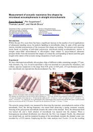
1. R. Barnkob, P. Augustsson, T. Laurell, <strong>and</strong> H. Bruus, Measurement <strong>of</strong><br />
acoustic resonance line shapes by microbead <strong>acoustophoresis</strong> in straight microchannels,<br />
USWNet 2009, 7th annual meeting, KTH-AlbaNova, 30 November<br />
– 1 December 2009, Stockholm, Sweden.<br />
2. P. Augustsson, R. Barnkob, C. Grenvall, T. Deierborg, P. Brundin, H.<br />
Bruus, <strong>and</strong> T. Laurell, Microchannel for measurements <strong>of</strong> acoustic properties<br />
<strong>of</strong> living cells, USWNet 2010, 8th annual meeting, 2-3 October 2010,<br />
Groningen, The Netherl<strong>and</strong>s.<br />
3. R. Barnkob, P. Augustsson, T. Laurell, <strong>and</strong> H. Bruus, Quantifying acoustic<br />
streaming in large-particle <strong>acoustophoresis</strong>, USWNet 2010, 8th annual<br />
meeting, 2-3 October 2010, Groningen, The Netherl<strong>and</strong>s.<br />
4. R. Barnkob, P. Augustsson, T. Laurell, <strong>and</strong> H. Bruus, An automated fullchip<br />
micro-PIV setup for measuring microchannel <strong>acoustophoresis</strong>: Simultaneous<br />
determination <strong>of</strong> forces from acoustic radiation <strong>and</strong> acoustic streaming,<br />
Proc. 14th MicroTAS, 3-7 October 2010, Groningen, The Netherl<strong>and</strong>s<br />
(S. Verporte, H. Andersson, J. Emneus, <strong>and</strong> N. Pamme, eds.), pp. 1247-49,<br />
CBMS, 2010.<br />
5. P. Augustsson, R. Barnkob, C. Grenvall, T. Deierborg, P. Brundin, H.<br />
Bruus, <strong>and</strong> T. Laurell, Measuring the acoustophoretic contrast factor <strong>of</strong><br />
living cells in microchannels. Proc. 14th MicroTAS, 3-7 October 2010,<br />
Groningen, The Netherl<strong>and</strong>s (S. Verporte, H. Andersson, J. Emneus, <strong>and</strong><br />
N. Pamme, eds.), pp. 1337-39, CBMS, 2010.<br />
6. C. L. Ebbesen, J. D. Adams, R. Barnkob, H. T. Soh, <strong>and</strong> H. Bruus,<br />
Temperature-controlled high-throughput (1 L/H) acoustophoretic particle separation<br />
in microchannels, Proc. 14th MicroTAS, 3-7 October 2010, Groningen,<br />
The Netherl<strong>and</strong>s (S. Verporte, H. Andersson, J. Emneus, <strong>and</strong> N.<br />
Pamme, eds.), pp. 728-30, CBMS, 2010.<br />
7. R. Barnkob, P. Augustsson, S. T. Wereley, H. Bruus, <strong>and</strong> T. Laurell, Microchannel<br />
<strong>acoustophoresis</strong>: continuous flow focusing efficiency compared to<br />
full-chip high-resolution micro-PIV measurements <strong>of</strong> the acoustic radiation<br />
force, International Congress on Ultrasonics, 5-8 September 2011, Gdansk,<br />
Pol<strong>and</strong>.<br />
8. R. Barnkob, P. Augustsson, C. Magnusson, H. Lilja, H. Bruus, <strong>and</strong> T. Laurell,<br />
Measuring density <strong>and</strong> compressibility <strong>of</strong> white blood cells <strong>and</strong> prostate<br />
cancer cells by microchannel <strong>acoustophoresis</strong>. Proc. 15th MicroTAS, 2-6<br />
October 2011, Seattle (WA), USA (J. L<strong>and</strong>ers, A. Herr, D. Juncker, N.<br />
Pamme, <strong>and</strong> J. Bienvenue, eds.), pp. 127-129, CBMS, 2011.
1.3 Publications during the PhD studies 7<br />
9. R. Barnkob, P. Augustsson, T. Laurell, <strong>and</strong> H. Bruus, Controlling the ratio<br />
<strong>of</strong> radiation <strong>and</strong> streaming forces in <strong>microparticle</strong> <strong>acoustophoresis</strong>, USWNet<br />
2012, 10th annual meeting, 21-22 September 2012, Lund, Sweden.<br />
10. P. Augustsson, R. Barnkob, H. Bruus, C. J. Kähler, T. Laurell, Á. G. Marín,<br />
P. B. Muller <strong>and</strong> M. Rossi, Measuring the 3D motion <strong>of</strong> particles in microchannel<br />
<strong>acoustophoresis</strong> using astigmatism particle tracking velocimetry,<br />
Proc. 16th MicroTAS, 28 October - 1 November 2012, Okinawa, Japan.<br />
11. M. Khoury, R. Barnkob, L. Laub Busk, P. Tidem<strong>and</strong>-Lichtenberg, H. Bruus,<br />
K. Berg-Sørensen, Optical stretching on chip with acoustophoretic prefocusing,<br />
SPIE Optics+Photonics, 12 - 16 August 2012, San Diego Convention<br />
Center, San Diego, California, USA.<br />
12. M. Rossi, R. Barnkob, P. Augustsson, Á. Márin, P. B. Muller, H. Bruus, T.<br />
Laurell <strong>and</strong> C. J. Kähler, Experimental <strong>and</strong> numerical characterization <strong>of</strong><br />
the 3D motion <strong>of</strong> particles in acoust<strong>of</strong>luidic devices, 3rd European Conference<br />
on Micr<strong>of</strong>ludics, 3-5 December 2012, Heidelberg, Germany.<br />
1.3.3 Conference abstracts<br />
1. R. Barnkob, P. Augustsson, T. Laurell, <strong>and</strong> H. Bruus, Decomposition <strong>of</strong><br />
acoustophoretic velocity fields into contributions from acoustic radiation <strong>and</strong><br />
acoustic streaming, DFS 2011, Danish Physical Society, 21-22 June 2011,<br />
Nyborg, Denmark<br />
2. R. Barnkob, P. Augustsson, T. Laurell, <strong>and</strong> H. Bruus, Particle-size dependent<br />
cross-over from radiation-dominated to streaming-dominated <strong>acoustophoresis</strong><br />
in microchannels, APS 2011, The 64th Annual Meeting <strong>of</strong> the<br />
Division <strong>of</strong> Fluid Dynamics, 20-22 November 2011, Baltimore, Maryl<strong>and</strong>,<br />
USA.<br />
3. M. J. H. Jensen, P. B. Muller, R. Barnkob, <strong>and</strong> H. Bruus, Numerical study<br />
<strong>of</strong> acoustic streaming <strong>and</strong> radiation forces on micro particles, BNAM 2012,<br />
Joint Baltic-Nordic Acoustics Meeting, June 18-20 2012, Odense, Denmark.<br />
4. H. Bruus, P. B. Muller, R. Barnkob, <strong>and</strong> M. J. H. Jensen, COMSOL analysis<br />
<strong>of</strong> acoustic streaming <strong>and</strong> <strong>microparticle</strong> <strong>acoustophoresis</strong>, COMSOL Conference<br />
Europe 2012, 10-12 October 2012, Milan, Italy.<br />
5. R. Barnkob, P. B. Muller, H. Bruus, <strong>and</strong> M. J. H. Jensen, Numerical analysis<br />
<strong>of</strong> radiation- <strong>and</strong> streaming-induced <strong>microparticle</strong> <strong>acoustophoresis</strong>, APS<br />
2012, The 65th Annual Meeting <strong>of</strong> the Division <strong>of</strong> Fluid Dynamics, 18-20<br />
November 2012, San Diego, California, USA.
8 Introduction
Chapter 2<br />
<strong>Physics</strong> <strong>of</strong> <strong>acoustophoresis</strong><br />
This chapter introduces the experimental <strong>acoustophoresis</strong> model system. This<br />
system represents a class <strong>of</strong> hard-material acoustic devices for generation <strong>of</strong> bulk<br />
acoustic resonances <strong>and</strong> it constitutes the basis for the analyses presented in this<br />
work. With the experimental model system in mind we describe the phenomena<br />
essential for underst<strong>and</strong>ing the acoustophoretic motion <strong>of</strong> <strong>microparticle</strong>s. This<br />
chapter provides an overview <strong>of</strong> the phenomena <strong>and</strong> their assumptions described<br />
in a qualitative manner rather than a more quantitative, mathematical description<br />
which is given in the following Chapter 3.<br />
2.1 Experimental model system<br />
Our experimental <strong>acoustophoresis</strong> model system was developed <strong>and</strong> is located in<br />
the lab <strong>of</strong> Pr<strong>of</strong>essor Thomas Laurell, Lund University, Sweden, <strong>and</strong> all experiments<br />
presented in this thesis using this system is carried out by or in collaboration<br />
with Dr. Per Augustsson. The core <strong>of</strong> the <strong>acoustophoresis</strong> system is a<br />
silicon/glass microchip attached to a piezoelectric transducer (piezo) responsible<br />
for the ultrasound actuation. The silicon/glass microchip is designed <strong>and</strong> fabricated<br />
by Dr. Per Augustsson <strong>and</strong> the reader is referred to his PhD thesis [18]<br />
<strong>and</strong> the Lab Chip Acoust<strong>of</strong>luidics 5 tutorial by Lensh<strong>of</strong> et al. for descriptions on<br />
the realization <strong>of</strong> such <strong>acoustophoresis</strong> devices [35].<br />
The experimental model system is shown in Fig. 2.1 <strong>and</strong> consists <strong>of</strong> a silicon/glass<br />
microchip translational invariant along its length L = 35 mm with an<br />
etched microchannel that can be loaded with particle suspension through silicone<br />
tuning at its ends. The chip is glued to <strong>and</strong> acoustically actuated by a piezo <strong>of</strong><br />
dimension 35 mm × 5 mm × 1 mm <strong>of</strong> the type Pz26 from Ferroperm Piezoceramics,<br />
Denmark. In Fig. 2.1(a) is shown a section along the length <strong>of</strong> the microchip<br />
showing the silicon chip (gray) <strong>of</strong> width W = 2.52 mm <strong>and</strong> height h si = 350 µm.
10 <strong>Physics</strong> <strong>of</strong> <strong>acoustophoresis</strong><br />
(a)<br />
x<br />
(d)<br />
y<br />
z<br />
Pyrex glass lid<br />
y<br />
Silicon chip base<br />
Microchannel<br />
(b)<br />
y<br />
Horizontal plane<br />
w/2<br />
x<br />
−w/2<br />
0 z l<br />
h/2<br />
(c) Vertical<br />
y<br />
cross section<br />
−h/2<br />
−w/2 w/2<br />
(e)<br />
Acoustophoresis<br />
microchip<br />
Outlet<br />
Peltier element<br />
Interrogation<br />
region<br />
Aluminum<br />
heat sink<br />
Temperature<br />
sensor<br />
Piezoceramic<br />
transducer<br />
Aluminum<br />
bar<br />
Inlet<br />
x [mm]<br />
-20<br />
2.52 mm<br />
-15<br />
0.38 mm<br />
-10<br />
-5<br />
0 5 10 15 20<br />
Figure 2.1: Experimental <strong>acoustophoresis</strong> model system located in the lab <strong>of</strong> Pr<strong>of</strong>essor<br />
Thomas Laurell, Lund University, Sweden, <strong>and</strong> developed <strong>and</strong> fabricated by Dr.<br />
Augustsson [18]. (a) A section <strong>of</strong> the <strong>acoustophoresis</strong> chip translational invariant along<br />
its length L consisting <strong>of</strong> a silicon chip base <strong>of</strong> width W <strong>and</strong> height h si , with an etched<br />
microchannel <strong>of</strong> width w <strong>and</strong> height h, <strong>and</strong> anodically bonded with a Pyrex glass lid <strong>of</strong><br />
width W <strong>and</strong> height h py . All chip <strong>and</strong> channel dimensions are listed in Table 2.1. (b)<br />
Horizontal xy plane section (magenta) at the channel mid height z = 0 <strong>of</strong> dimension<br />
l × w. (c) Vertical yz microchannel cross section (cyan) <strong>of</strong> dimension w × h. (d) Top<br />
view <strong>of</strong> the silicon chip base (dark gray), microchannel (blue), microscope field <strong>of</strong> view<br />
<strong>of</strong> length l (dashed white lines), <strong>and</strong> inlet <strong>and</strong> outlet tubing (light gray). (e) Photograph<br />
<strong>of</strong> the experimental model system placed in the automated <strong>and</strong> temperature-controlled<br />
micro-PIV setup described in Section 5.1. Particle suspensions are infused into the microchannel<br />
via the inlet <strong>and</strong> outlet silicone tubing <strong>and</strong> the chip is acoustically actuated<br />
by the piezoelectric transducer glued to the chip bottom. Adapted from Refs. [36, 37].<br />
The microchannel (light cyan) <strong>of</strong> width w = 377 µm <strong>and</strong> height h = 157 µm is<br />
etched into the silicon. The chip is anodically bonded with a Pyrex glass lid<br />
(transparent gray) <strong>of</strong> height h py = 1.13 mm. All chip <strong>and</strong> channel dimensions<br />
are summarized in Table 2.1. Throughout this thesis we place the origo O <strong>of</strong><br />
the spatial xyz coordinate system at the center <strong>of</strong> the microchannel such that x<br />
always points along the channel length, y along the transverse channel width, <strong>and</strong><br />
z along the channel height. Fig. 2.1(b) shows the horizontal xy plane (magenta)<br />
<strong>of</strong> dimension l × w at the channel mid height z = 0, where the length l refers to<br />
the width <strong>of</strong> a given microscope field <strong>of</strong> view. Fig. 2.1(c) shows the vertical yz<br />
microchannel cross section (cyan) <strong>of</strong> dimension w × h, while Fig. 2.1(d) shows<br />
a xy top view schematic <strong>of</strong> the silicon chip base (dark gray) <strong>and</strong> microchannel<br />
(blue).<br />
Fig. 2.1(e) shows a photograph <strong>of</strong> the experimental model system as it is placed<br />
in an automated <strong>and</strong> temperature-controlled setup described in Section 5.1. More<br />
information on the chip <strong>and</strong> setup can be found in Ref. [36] appended in Chap-
2.2 Acoustic actuation 11<br />
Table 2.1: Dimensions <strong>of</strong> the experimental model system shown in Fig. 2.1.<br />
Description Value Description Value<br />
Width, channel w 377 µm Width, chip W 2.52 mm<br />
Height, channel h 157 µm Height, silicon base h si 350 µm<br />
Length, channel L 35 mm Height, Pyrex glass lid h gl 1.13 mm<br />
Length, chip L 35 mm Height, chip h si + h gl 1.48 mm<br />
Piezo transducer (Pz26, Ferroperm, Denmark) 35 mm × 5 mm × 1 mm<br />
ter B.<br />
2.2 Acoustic actuation<br />
Basically, two ultrasound driving mechanisms are commonly used in acoust<strong>of</strong>luidics:<br />
(i) the generation <strong>of</strong> st<strong>and</strong>ing ultrasound bulk acoustic waves (BAW) driven<br />
by a piezo attached to the microchip acting as a resonator, see Fig. 2.1, <strong>and</strong> (ii)<br />
the generation <strong>of</strong> surface acoustic waves (SAW) by an interdigitated transducer<br />
on a piezoelectric substrate, see Refs. [19, 38, 39]. The two driving mechanisms<br />
are fundamentally different <strong>and</strong> each have their advantages, however, in this work<br />
we focus on BAW-driven <strong>acoustophoresis</strong>. Nevertheless, much <strong>of</strong> the fundamental<br />
physics remains the same, <strong>and</strong> it is the author’s hope that also researchers<br />
working on SAW-driven <strong>acoustophoresis</strong> can benefit from this thesis.<br />
As described in Section 2.1 our experimental model system supports BAWdriven<br />
<strong>acoustophoresis</strong>. The piezo is driven with a harmonic electric signal at<br />
low MHz frequencies sending MHz vibrations into the chip <strong>and</strong> the surroundings.<br />
These vibrations result in mm-wavelength acoustic resonances in the chip <strong>and</strong><br />
its liquid-filled cavities. These resonances lead to nonlinear interactions driving<br />
phenomena such as acoustic streaming <strong>of</strong> the suspending fluid <strong>and</strong> radiation forces<br />
on the suspended particles. In Fig. 2.2 is sketched the experimental model system<br />
<strong>and</strong> the involved phenomena arising from acoustically driving the system via the<br />
piezo. In the following we set out to describe these phenomena aiming at stating<br />
the underlying assumptions used in this thesis work to describe <strong>microparticle</strong><br />
<strong>acoustophoresis</strong>. The primary assumptions are listed in Table 2.2.<br />
2.2.1 Piezoelectric actuation<br />
A piezoelectric material transforms energy between electrical <strong>and</strong> mechanical<br />
forms such that an applied electric field generates mechanical stress <strong>and</strong> vice<br />
versa. At low voltages piezoelectric materials exhibit a linear relationship between<br />
electrical <strong>and</strong> mechanical energy <strong>and</strong> depending on the type <strong>of</strong> motion,<br />
scale <strong>of</strong> device, <strong>and</strong> material, it can be used to generate static <strong>and</strong> dynamic vibrations<br />
<strong>of</strong> up to hundreds <strong>of</strong> megahertz. Reviews on the use <strong>of</strong> piezoelectric<br />
transducers in acoust<strong>of</strong>luidics systems are given by Friend <strong>and</strong> Yeo [19] <strong>and</strong> in
12 <strong>Physics</strong> <strong>of</strong> <strong>acoustophoresis</strong><br />
Table 2.2: Primary theoretical assumptions used throughout the thesis.<br />
Microchannel fluid<br />
Piezo transducer<br />
Low amplitudes<br />
Isentropic oscillations<br />
Microchip<br />
Bulk acoustic waves<br />
St<strong>and</strong>ing waves<br />
Microparticles<br />
Single <strong>microparticle</strong>s<br />
Viscosity<br />
Acoustic streaming<br />
Constant parameters<br />
The microchannel contains a Newtonian <strong>and</strong> isotropic<br />
liquid.<br />
The geometry <strong>and</strong> resonance modes <strong>of</strong> the piezoelectric<br />
transducer are not treated <strong>and</strong> we assume harmonic<br />
time dependence <strong>of</strong> the lowest -order acoustic fields in<br />
the liquid.<br />
All acoustic amplitudes are low, i.e. the perturbation<br />
scheme is assumed to be valid.<br />
The acoustic oscillations <strong>of</strong> the microchannel liquid are<br />
assumed to be isentropic (adiabatic <strong>and</strong> reversible)<br />
processes [40].<br />
The geometry <strong>of</strong> the silicon/glass microchip has no<br />
influence on the acoustic resonances inside the<br />
liquid-filled microchannel, <strong>and</strong> instead the chip is<br />
modeled as hard-walled boundary conditions for the<br />
acoustic eigenmodes <strong>of</strong> the liquid-filled microchannel.<br />
The waves are bulk acoustic waves (BAW), i.e. all<br />
forms <strong>of</strong> surface acoustic waves (SAW) are neglected.<br />
The harmonic MHz actuation leads to the build-up <strong>of</strong><br />
acoustic resonances sufficiently fast to neglect the<br />
transient acoustic waves.<br />
All particles are spherical with radius a much smaller<br />
than the acoustic wavelength λ, i.e. a ≪ λ.<br />
The particle suspensions are dilute enough to neglect<br />
any hydrodynamic as well as acoustic particle-particle<br />
interactions.<br />
Viscosity is considered to be negligible in the bulk <strong>of</strong><br />
the fluid, but non-negligible near solid surfaces such as<br />
particles <strong>and</strong> walls, where the fluid velocity gradients<br />
are large inside the viscous boundary layers.<br />
We only treat boundary-driven acoustic streaming <strong>and</strong><br />
hence we neglect other types <strong>of</strong> acoustic streaming<br />
such as bulk attenuation-driven streaming <strong>and</strong><br />
cavitation microstreaming around bubbles.<br />
The following parameters are assumed to be constant:<br />
• viscosity η,<br />
• heat conductivity k th ,<br />
• specific heats C p <strong>and</strong> C v ,<br />
• compressibility κ,<br />
• thermal expansion α.
2.2 Acoustic actuation 13<br />
Figure 2.2: Sketch <strong>of</strong> the physics <strong>of</strong> <strong>acoustophoresis</strong> in our experimental model<br />
system shown in Fig. 2.1. (a) The microchip (gray) is attached to the piezo (brown) via<br />
an acoustic coupling layer (green). The piezo is driven harmonically at MHz frequencies<br />
giving rise to resonances building up in the bulk <strong>of</strong> the chip <strong>and</strong> inside the liquidfilled<br />
microchannel. (b) Zoom-in on the liquid-filled microchannel (light blue) with an<br />
imposed acoustic transverse st<strong>and</strong>ing half wave (red). The liquid oscillations must fulfill<br />
the no-slip condition at the solid walls resulting in the creation <strong>of</strong> a thin thermoviscous<br />
boundary layer (intermediate blue). Inside the boundary layer arise acoustic streaming<br />
rolls (dark blue) which drive acoustic streaming rolls in the bulk liquid (dark blue). (c)<br />
Microparticles (•) suspended in the channel is primarily subject to two forces (i) drag<br />
forces from the induced acoustic streaming <strong>and</strong> (ii) acoustic radiation forces emanating<br />
from the scattering <strong>of</strong> waves.<br />
the tutorial paper by Dual <strong>and</strong> Möller [41] outlining the piezoelectric <strong>theory</strong> <strong>and</strong><br />
its applicability when designing acoust<strong>of</strong>luidic devices.<br />
As pointed out in the reviews, the electric actuation <strong>of</strong> the piezoelectric material<br />
is complicated, making model predictions difficult. In piezoelectric materials<br />
the mechanical <strong>and</strong> electrical behavior are coupled such that a change in electrical<br />
boundary conditions will change the material’s mechanical behavior <strong>and</strong> vice<br />
versa, e.g. mechanical loading or damping <strong>of</strong> a piezoelectric material will tend<br />
to increase its electrical impedance. The mechanical loading depends on all connected<br />
device elements, <strong>and</strong> in our systems, in particular, the coupling glue layer<br />
between chip <strong>and</strong> transducer. This glue layer is <strong>of</strong>ten more or less <strong>of</strong> r<strong>and</strong>om homogeneity<br />
<strong>and</strong> thickness making theoretical predictions <strong>of</strong> the coupling difficult.
14 <strong>Physics</strong> <strong>of</strong> <strong>acoustophoresis</strong><br />
Moreover, theoretical predictions could also take into account the damping <strong>of</strong> the<br />
piezoelectric transducer due to the surrounding air <strong>and</strong> experimental platform on<br />
which it rests. On the other h<strong>and</strong>, due to the electromechanical coupling one can<br />
use electrical measurements like admittance curves to experimentally characterize<br />
acoust<strong>of</strong>luidics devices as described by Dual et al. [42]. Admittance curves<br />
can be used for e.g. detecting resonance frequencies if the system <strong>and</strong> transducer<br />
resonances match reasonably well [41].<br />
In this work we do not try to predict the behavior <strong>of</strong> the piezoelectric element<br />
as this would require a better control <strong>of</strong> the actual coupling layer between chip<br />
<strong>and</strong> transducer <strong>and</strong> the damping from the experimental platform consisting <strong>of</strong><br />
temperature control elements etc. should then be taken into account. Instead we<br />
simply assume that the liquid-filled microchannel experiences a harmonic acoustic<br />
actuation in its bulk, disregarding any boundary actuation effects which would<br />
be the result <strong>of</strong> a deeper analysis <strong>of</strong> the piezoelectric actuation <strong>and</strong> the mechanics<br />
<strong>of</strong> the solid chip materials. Furthermore, we assume the harmonic actuation to<br />
be <strong>of</strong> reasonably low amplitude 1 in order to apply a perturbation scheme in the<br />
mathematical analysis described in Chapter 3.<br />
2.2.2 Ultrasound resonances<br />
The microchip sketched in Fig. 2.2 forms an acoustic resonator implying that<br />
acoustic resonances occurs at specific frequencies f j . Here a resonance is the<br />
tendency <strong>of</strong> the system to oscillate at greater amplitudes at some frequencies f j<br />
than at other frequencies f ≠ f j , such that the acoustic energy density inside<br />
the resonator becomes several orders <strong>of</strong> magnitude larger at resonance. Besides<br />
oscillating at large amplitudes, the resonance modes are usually both stable <strong>and</strong><br />
reproducible <strong>and</strong> their spatial pattern are set by the geometry <strong>of</strong> the system<br />
[43]. Hence, the piezoelectric transducer is operated at frequencies f close to<br />
the system’s resonance frequencies f j <strong>and</strong> as close as possible to the resonances<br />
<strong>of</strong> the piezo to allow optimal coupling <strong>of</strong> the transmitted acoustic energy. The<br />
microchannel in the experimental model system is therefore designed to support<br />
a horizontal transverse resonance at 2 MHz, which is the resonance frequency <strong>of</strong><br />
the piezo.<br />
To underst<strong>and</strong> this type <strong>of</strong> systems it is important to avoid thinking in terms<br />
<strong>of</strong> traveling waves. For example, in glass a 2-MHz ultrasound wave propagates<br />
for around 200 µs corresponding to a length <strong>of</strong> 1.1 m before it dies out due to<br />
intrinsic attenuation. Thus, in our mm-sized microchip this wave experiences<br />
∼1000 reflections <strong>and</strong> the spatial pattern <strong>of</strong> a resonance mode is therefore set by<br />
the geometry <strong>and</strong> frequency rather than the spatial behavior <strong>of</strong> the actuation.<br />
The precise frequency <strong>of</strong> a desired microchannel resonance mode depends on<br />
the whole surrounding system <strong>and</strong> the coupling to the piezo. Such models are<br />
described in the recent tutorial by Dual <strong>and</strong> Möller [41], where they establish a<br />
1 Using the Ferroperm Piezoelectric calculator (http://www.ferroperm-piezo.com/) we obtain<br />
a 7-nm actuation amplitude when exciting an unloaded 35 mm×5 mm×1 mm-large Pz26 element<br />
at 20 V peak-to-peak voltage.
2.2 Acoustic actuation 15<br />
numerical model integrating the piezoelectric <strong>theory</strong> with the elastic wave <strong>theory</strong><br />
for the solid chip materials [9, 44], <strong>and</strong> the acoustic fluid waves inside the microchannel<br />
[43, 45]. However, such fully-integrated models are numerically timeconsuming<br />
for realistic system dimensions <strong>and</strong> furthermore some experimental<br />
conditions, such as the coupling glue layer thickness <strong>and</strong> homogeneity, are too<br />
ill-defined.<br />
In this work we will use first-order linear fluid <strong>theory</strong> to analyze the acoustic<br />
resonances (eigenmodes) <strong>of</strong> the microchannel <strong>and</strong> represent the surrounding chip<br />
by approximate boundary conditions. Furthermore, the bulk viscous (<strong>and</strong> thermal)<br />
attenuation is negligible <strong>and</strong> we therefore treat inviscid bulk acoustics [43].<br />
Contrary in the bulk liquid, viscosity does play a significant role near the solid<br />
boundaries where the fluid must satisfy the no-slip velocity condition resulting<br />
in the presence <strong>of</strong> a sub-µm-thin thermoviscous boundary layer containing large<br />
fluid velocity gradients [45].<br />
2.2.3 Non-linear effects<br />
As sketched in Fig. 2.2 the acoustic resonances in the fluid drive two non-linear<br />
effects known as acoustic streaming <strong>and</strong> acoustic radiation forces. While the<br />
linear effects <strong>of</strong> the acoustic resonance time averages to zero (average over one<br />
period <strong>of</strong> harmonic oscillation, typically ∼ 1 µs), the non-linear effects lead to<br />
non-zero time-averaged forces on the fluid <strong>and</strong> the suspended particles.<br />
2.2.3.1 Acoustic streaming<br />
Acoustic streaming is the generation <strong>of</strong> flow from sound <strong>and</strong> is a well-known phenomenon<br />
within the studies <strong>of</strong> acoustics. Acoustic streaming appears in different<br />
forms, but common to all <strong>of</strong> them is the appearance <strong>of</strong> a steady fluid flow driven<br />
by viscous attenuation <strong>of</strong> acoustic waves. In viscous fluids the viscous attenuation<br />
causes a net displacement <strong>of</strong> fluid particles resulting in streaming flows. For an<br />
ideal inviscid fluid the small acoustic oscillations <strong>of</strong> the fluid are reversible <strong>and</strong><br />
hence the time-average net flow is zero.<br />
In acoust<strong>of</strong>luidic systems the viscous attenuation driving the streaming <strong>of</strong>ten<br />
takes place in either the bulk fluid or in the viscous boundary layers near solid<br />
walls. Other forms are the cavitation microstreaming driven by bubble oscillations<br />
[46] <strong>and</strong> streaming driven in surface acoustic wave systems [47]. In this work<br />
we deal only with boundary-induced acoustic streaming as we treat bulk acoustic<br />
waves in a system with ideally no bubbles <strong>and</strong> a length scale much smaller than<br />
the viscous attenuation length required for bulk-induced streaming [11]. For more<br />
information on the applications <strong>of</strong> the different forms <strong>of</strong> streaming in microsystems,<br />
the reader is referred to Refs. [11, 47], while a more thorough theoretical<br />
review can be found in Refs. [48–50]. To clarify, in this thesis we only consider<br />
boundary-induced acoustic streaming <strong>and</strong> the term acoustic streaming refers to<br />
this streaming form only.
16 <strong>Physics</strong> <strong>of</strong> <strong>acoustophoresis</strong><br />
Boundary-induced acoustic streaming is a steady rotational motion <strong>of</strong> an oscillating<br />
fluid close to a solid boundary. At the solid boundaries the oscillating<br />
fluid velocity must go to zero to fulfill the no slip condition from molecular forces<br />
between the solid boundary <strong>and</strong> the molecules <strong>of</strong> the fluid. This decay <strong>of</strong> the oscillating<br />
fluid velocity happens on a length scale denoted the viscous acoustic boundary<br />
layer thickness δ. For a st<strong>and</strong>ing wave parallel to a solid plane boundary, the<br />
viscous attenuation drives a momentum flux close to the boundary from the pressure<br />
antinodes to the pressure nodes [47] resulting in a steady vorticity inside<br />
the viscous boundary layer termed inner streaming rolls (also Schlichting rolls),<br />
which were first treated by Schlichting in 1932 based on Pr<strong>and</strong>tl’s boundary-layer<br />
<strong>theory</strong> [51]. The inner streaming rolls drive the counter-rotating streaming rolls<br />
in the bulk fluid referred to as the outer streaming rolls (or Rayleigh rolls), which<br />
were first described theoretically by Rayleigh in 1884, who derived the expression<br />
for the fluid slip velocity just outside the viscous boundary layer [52]. Both the<br />
inner <strong>and</strong> outer streaming rolls are sketched in Fig. 2.2.<br />
2.2.3.2 Acoustic radiation forces<br />
The acoustic radiation force is the key parameter in most acoust<strong>of</strong>luidic applications<br />
<strong>and</strong> in particular when dealing with acoustic particle <strong>and</strong> cell manipulation.<br />
The acoustic radiation force arises from scattering <strong>of</strong> the acoustic waves on particles<br />
suspended in a fluid with an imposed acoustic field. This scattering causes a<br />
momentum transfer from the acoustic wave to the suspended particles resulting<br />
in a net radiation force that cause a migration <strong>of</strong> the particles relative to the<br />
suspending fluid.<br />
2.2.4 Acoustophoretic particle motion<br />
As illustrated in Fig. 2.2(c) particles suspended in the liquid inside the microchannel<br />
are influenced by the acoustic actuation as they become subject to streaminginduced<br />
drag forces from the suspending liquid <strong>and</strong> the acoustic radiation forces<br />
acting directly on them due to scattering. Throughout the thesis, we base our<br />
analysis on these two effects. We neglect any particle-particle effects, hydrodynamic<br />
as well as acoustic. Regarding the hydrodynamic interactions, Mikkelsen<br />
<strong>and</strong> Bruus [53] reported that hydrodynamic effects become significant for interparticle<br />
distances below 2 particle diameters <strong>and</strong> hence we will keep the experiments<br />
well above this threshold. The acoustically induced inter-particle effects<br />
arise from waves that scatters from one particle onto another <strong>and</strong> hence it is <strong>of</strong>ten<br />
denoted the secondary radiation force or Bjerknes forces. However, for solid<br />
particles (<strong>and</strong> not bubbles) the Bjerknes forces are negligible in comparison to<br />
the primary radiation force <strong>and</strong> the hydrodynamic particle-particle effects [54]. A<br />
primary assumption is therefore that we consider particle suspensions such dilute<br />
that particle-particle effects are negligible. Also, where not otherwise stated, the<br />
influence <strong>of</strong> the walls on the viscous drag coefficients is neglected.
2.3 Concluding remarks 17<br />
2.3 Concluding remarks<br />
This chapter introduced the experimental model system that forms the basis for<br />
the analyses in the thesis. With the experimental model system in focus, the<br />
phenomena arising from acoustic actuation were introduced <strong>and</strong> in Table 2.2<br />
the primary theoretical assumptions were summarized <strong>and</strong> used to establish the<br />
theoretical framework presented in the next Chapter 3.
18 <strong>Physics</strong> <strong>of</strong> <strong>acoustophoresis</strong>
Chapter 3<br />
Theory <strong>of</strong> <strong>acoustophoresis</strong><br />
In this chapter the theoretical framework for the thesis is introduced, namely<br />
the <strong>theory</strong> <strong>of</strong> the involved physics <strong>and</strong> approximations described in the former<br />
Chapter 2. The presented <strong>theory</strong> is classical <strong>and</strong> well known dating back to the<br />
time <strong>of</strong> Helmholtz <strong>and</strong> Lord Rayleigh, <strong>and</strong> the approach presented here is inspired<br />
mainly by L<strong>and</strong>au <strong>and</strong> Lifshitz [45, 55], Pierce [40], <strong>and</strong> Bruus [43, 56].<br />
Vectors, tensors, <strong>and</strong> derivatives<br />
All symbols <strong>and</strong> acronyms are listed in the List <strong>of</strong> Symbols <strong>and</strong> Acronyms on<br />
page xiv. However, parts <strong>of</strong> the notation require a little more description:<br />
Vectors <strong>and</strong> tensors. Vectors are represented as bold symbols or by index<br />
notation <strong>and</strong> the Einstein summation convention, e.g., v i , where i is the i’th<br />
spatial vector component (x, y, <strong>and</strong> z) <strong>and</strong> where repeated indices indicate a<br />
summation over the index. Especially, we mostly represent tensors using the<br />
index notation for clarity about which index a given operater acts on.<br />
Derivatives. Derivatives are represented by the short notation, i.e. ∂ i ≡ ∂ . ∂i<br />
3.1 Governing equations <strong>of</strong> a thermoviscous fluid<br />
We study the motion <strong>of</strong> a Newtonian fluid. The fluid is regarded as a continuous<br />
medium, i.e. we consider the motion <strong>of</strong> fluid particles that contain a large number<br />
<strong>of</strong> molecules (continuum hypothesis). In order to describe this motion, we use<br />
the Eulerian description <strong>of</strong> any fluid field F = F (r, t), i.e., the position r <strong>and</strong><br />
time t are independent variables.<br />
The state <strong>of</strong> a moving, compressible, <strong>and</strong> thermoviscous fluid is completely<br />
determined by the three components <strong>of</strong> the fluid velocity v, <strong>and</strong> any two <strong>of</strong> the<br />
thermodynamic quantities, e.g., the temperature T <strong>and</strong> the pressure p [45]. All
20 Theory <strong>of</strong> <strong>acoustophoresis</strong><br />
the remaining thermodynamic quantities are thus to be determined through the<br />
equations <strong>of</strong> state. The mathematical description <strong>of</strong> the state <strong>of</strong> the moving fluid<br />
is therefore fully described by the equations <strong>of</strong> conservation <strong>of</strong> mass, momentum<br />
<strong>and</strong> energy.<br />
Conservation <strong>of</strong> mass. The mass conservation equation <strong>of</strong> the fluid is the<br />
continuity equation [45]<br />
∂ t ρ = − ∇ · (ρv) , (3.1)<br />
where ρ is the fluid mass density. In this thesis we deal with acoustics which<br />
is essentially propagation <strong>of</strong> compression <strong>and</strong> decompression, hence the fluid is<br />
treated as compressible ∇ · v ≠ 0.<br />
Conservation <strong>of</strong> momentum. The equation for conservation <strong>of</strong> momentum<br />
is the Navier–Stokes equation [45]<br />
ρ [∂ t v i + (v j ∂ j ) v i ] = −∂ i p + ∂ j σ ′ ij, (3.2)<br />
where we have neglected any external forces, <strong>and</strong> where we have introduced the<br />
viscous stress tensor σ ′ with the ij’th component<br />
σ ′ ij = η (∂ j v i + ∂ i v j ) + (β − 1)η (∂ k v k ) δ ij . (3.3)<br />
Here δ ij is the Kronecker delta <strong>and</strong> η is the fluid dynamic viscosity. Moreover, we<br />
have introduced the compressional viscosity ratio β = ζ/η + 1/3, where ζ is the<br />
so-called second coefficient <strong>of</strong> viscosity, also called the bulk viscosity or expansion<br />
viscosity (losses due to compression <strong>and</strong> expansion <strong>of</strong> the fluid). In this work we<br />
use ζ = 0 ⇒ β = 1/3 as <strong>of</strong> simple liquids [57].<br />
Conservation <strong>of</strong> energy. The law <strong>of</strong> conservation <strong>of</strong> energy is governed by<br />
the so-called heat-transfer equation [45]<br />
∂ t<br />
( 1<br />
2 ρv2 + ρɛ ) = − ∇ · [v ( 1<br />
2 ρv2 + ρɛ + p ) − v · σ ′ − k th ∇T ] , (3.4)<br />
where ɛ is the internal energy per unit mass, T is the temperature, <strong>and</strong> k th is the<br />
thermal conductivity. In terms <strong>of</strong> the entropy per unit mass s, the equation can<br />
be rewritten as [45]<br />
ρT [∂ t s + (v · ∇) s] = σ ′ ik∂ i v k + ∇ · (k th ∇T ) . (3.5)<br />
Defining constants. As described in the assumptions in Table 2.2 we neglect<br />
any spatial variations in the fluid viscosities η <strong>and</strong> thermal conduction k th as well<br />
as any variations in the fluid’s compressibility κ, speed <strong>of</strong> sound c, heat capacities<br />
C p <strong>and</strong> C v , <strong>and</strong> thermal expansion α. However, for second-order acoustics, it<br />
turns out that the variations in viscosity with temperature plays a significant role<br />
for, e.g. acoustic streaming, as discussed in Section 3.4 <strong>and</strong> Ref. [58]. With constant<br />
viscosity <strong>and</strong> thermal conductivity, the governing equations <strong>of</strong> conservation<br />
become<br />
∂ t ρ = −∇ · (ρv) ,<br />
ρ [∂ t v + (v · ∇) v] = −∇p + η∇ 2 v + βη∇ (∇ · v) ,<br />
ρT [∂ t s + (v · ∇) s] = σ ′ ik∂ i v k + k th ∇ 2 T.<br />
(3.6a)<br />
(3.6b)<br />
(3.6c)
3.1 Governing equations <strong>of</strong> a thermoviscous fluid 21<br />
3.1.1 Thermodynamic relations<br />
We describe the thermodynamic quantities by means <strong>of</strong> the temperature T <strong>and</strong><br />
the pressure p, <strong>and</strong> thus we can describe the changes in the density ρ = ρ (T, p)<br />
<strong>and</strong> entropy per mass s = s (T, p) as<br />
dρ = (∂ T ρ) p<br />
dT + (∂ p ρ) T<br />
dp,<br />
ds = (∂ T s) p<br />
dT + (∂ p s) T<br />
dp.<br />
(3.7a)<br />
(3.7b)<br />
Here, (∂ p ρ) T<br />
= γ (∂ p ρ) s<br />
= (γ/c 2 ) = γρκ, where γ = C p /C v is the ratio <strong>of</strong> the<br />
specific heats C p at constant pressure <strong>and</strong> C v at constant volume, 1/c 2 = (∂ p ρ) s<br />
is one over the square <strong>of</strong> the isentropic speed <strong>of</strong> sound, <strong>and</strong> κ = 1/ (ρc 2 ) is<br />
the isentropic compressibility [40]. Further, we use the definition <strong>of</strong> the isobaric<br />
thermal expansion α = − (1/ρ) (∂ T ρ) p<br />
to write (∂ T ρ) p<br />
= −αρ, the definition<br />
<strong>of</strong> the specific heat C p to get (∂ T s) p<br />
= C p /T <strong>and</strong> lastly the Maxwell relation<br />
(∂ p s) T<br />
= − [ ( )]<br />
∂ 1<br />
T = − (α/ρ) [55]. We thus end up with the two general<br />
ρ p<br />
thermodynamic identities<br />
dρ = γρκ dp − αρ dT,<br />
ds = C p<br />
T dT − α ρ dp.<br />
(3.8a)<br />
(3.8b)<br />
In the isentropic case ds = 0, the identities reduce to<br />
where we have used the thermodynamic identity [55]<br />
dp = ρC p<br />
αT dT = c2 dρ, (3.9)<br />
γ = T α2<br />
+ 1. (3.10)<br />
ρC p κ<br />
3.1.2 Perturbation scheme<br />
As described in Table 2.2, we assume an acoustic wave to constitute tiny perturbations<br />
to a zeroth-order state <strong>of</strong> the liquid. At its zeroth-order state the liquid is<br />
homogeneous, quiescent, <strong>and</strong> in thermal equilibrium, such that the zeroth-order<br />
fields become T 0 , p 0 , v 0 = 0, ρ 0 , <strong>and</strong> s 0 . By taking first- <strong>and</strong> second-order perturbations<br />
(subscript 1 <strong>and</strong> 2, respectively) into account, we write the perturbation<br />
series as<br />
p = p 0 + p 1 + p 2 , v = 0 + v 1 + v 2 , T = T 0 + T 1 + T 2 , (3.11a)<br />
ρ = ρ 0 + ρ 1 + ρ 2 , s = s 0 + s 1 + s 2 , (3.11b)<br />
where the perturbation parameter is implicitly assumed, i.e. T 0 ≫ T 1 ≫ T 2 .
22 Theory <strong>of</strong> <strong>acoustophoresis</strong><br />
3.1.3 Thermoviscous first-order equations<br />
To first order in the acoustic perturbations we use the thermodynamic identities in<br />
Eqs. (3.8a) <strong>and</strong> (3.8b) to eliminate ρ 1 <strong>and</strong> s 1 resulting in the following expressions<br />
for the continuity equation expressed in terms <strong>of</strong> p 1 , the Navier–Stokes equation<br />
for v 1 , <strong>and</strong> the thermodynamic heat-transfer equation for T 1<br />
∂ t p 1 = 1<br />
γκ (α∂ tT 1 − ∇ · v 1 ) ,<br />
(3.12a)<br />
ρ 0 ∂ t v 1 = −∇p 1 + η∇ 2 v 1 + βη∇ (∇ · v 1 ) ,<br />
(3.12b)<br />
∂ t T 1 = D th ∇ 2 T 1 + αT 0<br />
ρ 0 C p<br />
∂ t p 1 ,<br />
where we have introduced the thermal diffusivity<br />
(3.12c)<br />
D th =<br />
k th<br />
ρ 0 C p<br />
. (3.13)<br />
As outlined in Chapter 2 we assume all first-order fields to be harmonic in time,<br />
i.e. F (r, t) = F (r) exp (−iωt). We get ∂ t p 1 = −iωp 1 <strong>and</strong> we can eliminate p 1<br />
from Eq. (3.12)<br />
iωv 1 + ν∇ 2 v 1 +<br />
[<br />
νβ +<br />
i ]<br />
∇ (∇ · v<br />
γρ 0 κω<br />
1 ) =<br />
α<br />
γρ 0 κ ∇T 1,<br />
(3.14a)<br />
iωT 1 + γD th ∇ 2 T 1 = γ − 1<br />
α ∇ · v 1. (3.14b)<br />
From Eq. (3.14) arise the thermal <strong>and</strong> the viscous boundary layer thicknesses δ th<br />
<strong>and</strong> δ [45], respectively (values for 2-MHz ultrasound waves in water at 25 ◦ C),<br />
δ th =<br />
√<br />
2γDth<br />
ω<br />
= 0.15 µm, (3.15a)<br />
δ =<br />
√<br />
2ν<br />
ω<br />
= 0.38 µm. (3.15b)<br />
These are the length scales over which the acoustic fields change from their values<br />
in the bulk to their values at rigid boundaries.<br />
3.1.4 Isentropic first-order equations<br />
Throughout the thesis (except Chapter 4) we assume the acoustic oscillations to<br />
be isentropic, such that ds = 0 [40] <strong>and</strong> Eq. (3.12) reduces to<br />
ρ 0 ∂ t v 1 = −∇p 1 + η∇ 2 v 1 + βη∇ (∇ · v 1 ) ,<br />
1<br />
c ∂ tp 2 1 = −ρ 0 ∇ · v 1 ,<br />
ρ 1 = 1 c 2 p 1,<br />
(3.16a)<br />
(3.16b)<br />
(3.16c)<br />
T 1 = αT 0<br />
ρ 0 C p<br />
p 1 .<br />
(3.16d)
3.1 Governing equations <strong>of</strong> a thermoviscous fluid 23<br />
Thus, we can solve Eqs. (3.16a) <strong>and</strong> (3.16b) for v 1 <strong>and</strong> p 1 , <strong>and</strong> ρ 1 <strong>and</strong> T 1 are<br />
then given by inserting p 1 into Eqs. (3.16c) <strong>and</strong> (3.16d), respectively.<br />
3.1.4.1 Acoustic wave equation<br />
If we take the time derivative <strong>of</strong> Eq. (3.16b) <strong>and</strong> insert Eq. (3.16a) we obtain for<br />
p 1 the acoustic wave equation (with an extra term due to viscous attenuation)<br />
[<br />
]<br />
1<br />
c ∂ 2 t 2 (1 + β) η<br />
p 1 = 1 − ∂<br />
ρ 0 c 2 t ∇ 2 p 1 . (3.17)<br />
Further, with the harmonic time dependence <strong>of</strong> p 1 we get the so-called lossy<br />
Helmholtz wave equation<br />
∇ 2 p 1 = −k 2 (1 + iγ att ) p 1 ,<br />
γ att =<br />
(3.18a)<br />
(1 + β) ηω<br />
2ρ 0 c 2 , (3.18b)<br />
where we have introduced the wavenumber k = ω/c <strong>and</strong> the viscous damping<br />
coefficient γ att which is assumed to be small since γ att ≈ 10 −6 for 2-MHz ultrasound<br />
oscillations in water at 25 ◦ C. Possible solutions to the lossy Helmholtz<br />
wave equation are damped plane waves<br />
p 1 (r, t) = p a e i(k·r−ωt) e −γ att k·r , (3.19)<br />
where p a is the undamped amplitude <strong>of</strong> the wave <strong>and</strong> where the real exponential<br />
term with γ att constitutes the damping <strong>of</strong> the wave. The characteristic damping<br />
length 1/ (γ att k) ≈ 36 m is very long for our micr<strong>of</strong>luidic system <strong>and</strong> hence<br />
we neglect all bulk viscous attenuation. Thus, in the invicid case Eq. (3.17)<br />
reduces to the wave equation ∇ 2 p 1 = (1/c 2 )∂ 2 t p 1 with the general 1D solution<br />
p 1 = p 1 (x ± ct) showing that c is indeed the (isentropic) speed <strong>of</strong> sound <strong>of</strong> the<br />
fluid. The inviscid case further leads to v 1 being irrotational <strong>and</strong> hence being the<br />
gradient <strong>of</strong> a potential v 1 ≡ ∇φ, <strong>and</strong> we can relate the velocity v 1 , the pressure<br />
p 1 , density ρ 1 , <strong>and</strong> the temperature T 1 as<br />
v 1 = − i<br />
ρ 0 ω ∇p 1 = − ic2<br />
ρ 0 ω ∇ρ 1 = − ic2 C p<br />
ωαT 0<br />
∇T 1 . (3.20)<br />
3.1.5 Second-order equations<br />
In the linear first-order <strong>theory</strong> all fields are harmonically varying in time resulting<br />
in no time-average contribution. Therefore in order to obtain time-averaged<br />
effects we go to the second-order perturbations, where we for simplicity neglect<br />
the second-order temperature T 2 <strong>and</strong> stay in the isentropic regime. Hence, we are<br />
left with the time-averaged second-order continuity equation <strong>and</strong> Navier–Stokes<br />
equation [59]<br />
ρ 0 ∇ · 〈v 2 〉 = −∇ · 〈ρ 1 v 1 〉,<br />
η∇ 2 〈v 2 〉 + βη∇ (∇ · 〈v 2 〉) − 〈∇p 2 〉 = 〈ρ 1 ∂ t v 1 〉 + ρ 0 〈(v 1 · ∇) v 1 〉.<br />
(3.21a)<br />
(3.21b)
24 Theory <strong>of</strong> <strong>acoustophoresis</strong><br />
Notice that the products <strong>of</strong> first-order fields act as source terms for the secondorder<br />
fields v 2 <strong>and</strong> p 2 . The second-order pressure p 2 contributes to the acoustic<br />
radiation forces <strong>and</strong> the second-order velocity v 2 is responsible for the acoustic<br />
streaming as described later in Sections 3.3 <strong>and</strong> 3.4, respectively.<br />
3.1.6 Acoustic energy density<br />
The acoustic energy density is an essential parameter in <strong>microparticle</strong> <strong>acoustophoresis</strong><br />
as it sets the scale for the acoustic radiation forces <strong>and</strong> streaming flows.<br />
The energy transported with acoustic waves is composed <strong>of</strong> the kinetic energy<br />
<strong>of</strong> the moving fluid elements <strong>and</strong> the potential energy <strong>of</strong> the compressed fluid.<br />
The kinetic energy density is given by the st<strong>and</strong>ard formulation E kin = (1/2)ρ 0 v1,<br />
2<br />
while the potential energy density is derived from the energy stored due to compression<br />
<strong>and</strong> expansion E pot = − ´ V<br />
V 0<br />
(p 1 /V )dV = (1/2)κp 2 1 [60]. Hence, the total<br />
time-averaged acoustic energy density E ac (r) becomes<br />
E ac (r) = 1 2 ρ 0〈v 2 1〉 + 1 2 κ〈p2 1〉 = 1 4<br />
(<br />
ρ0 v 2 1 + κp 2 1<br />
)<br />
, (3.22)<br />
where we have used the relation <strong>of</strong> the time average <strong>of</strong> the product <strong>of</strong> two timeharmonic<br />
fields 〈A(t)B(t)〉 = 1 2 Re { A (0) ¯B (0) } , where the bar represents complex<br />
conjugation.<br />
3.2 Resonances<br />
As discussed in Chapter 2 the resonances in the microchannel <strong>of</strong> our experimental<br />
model system depends on the actuation <strong>of</strong> the piezo, the coupling glue layer<br />
between piezo <strong>and</strong> chip, the mechanical loading <strong>of</strong> the piezo, <strong>and</strong> the chip <strong>and</strong><br />
channel materials <strong>and</strong> geometries. In this work, however, we use a simple model<br />
to describe the resonances inside the liquid-filled microchannel neglecting any<br />
interaction with the bulk chip <strong>and</strong> the spatial behavior <strong>of</strong> the piezo actuation.<br />
Mathmatically, resonance means that a system gets into its eigenmode where<br />
the acoustic energy density becomes unbounded, but if small losses are present<br />
the energy density will be bounded but be very large. In the following we study<br />
the eigenmodes for the liquid-filled microchannel <strong>and</strong> describe the associated resonance<br />
spectrum.<br />
3.2.1 Eigenmodes for a liquid rectangular cuboid<br />
In the following we model the liquid-filled microchannel <strong>of</strong> experimental model<br />
system as a liquid-filled rectangular cuboid where its boundary conditions represent<br />
the surrounding chip. Furthermore, we presume that the chip materials are
3.2 Resonances 25<br />
Figure 3.1: Pressure eigenmode p 1 (from p a (dark red) to −p a (dark blue)),<br />
Eq. (3.24), for a liquid rectangular cuboid surrounded by infinitely hard walls <strong>and</strong><br />
dimensions similar to the microchannel ) in the experimental model system, Fig. 2.1.<br />
The eigenmode has<br />
(n x , n y , n z = (20, 1, 0) <strong>and</strong> only the channel fraction <strong>of</strong> 2 mm<br />
around x = 0 is shown. (a) 3D slice plot <strong>of</strong> the eigenmode p 1 . (b) The eigenmode<br />
pressure in the vertical yz microchannel cross section at x = 0. (c) The eigenmode<br />
pressure in the horizontal xy plane at channel mid height z = 0.<br />
acoustically infinitely hard in comparison to the liquid channel 1 to apply hard wall<br />
conditions at all boundaries, i.e. n·∇p| y=±w/2 = n·∇p| z=±h/2 = n·∇p| x=±L/2 =<br />
0. By solving the Helmholtz wave equation Eq. (3.18a) (γ att = 0) with these conditions,<br />
we get the following eigenfrequencies<br />
f nx ,n y ,n z<br />
= c 0<br />
2<br />
√<br />
n 2 x<br />
l + n2 y<br />
2 w + n2 z<br />
2 h , with n x, n 2 y , n z = 0, 1, 2, 3, . . . , (3.23)<br />
where the three indexes n x , n y , n z are the number <strong>of</strong> half-wavelengths along x, y,<br />
<strong>and</strong> z, respectively. The corresponding eigenfunction p 1 becomes<br />
(<br />
p 1 (x, y, z) = p a cos<br />
[k x x + L )] (<br />
cos<br />
[k<br />
2<br />
y y + w )] (<br />
cos<br />
[k<br />
2<br />
z z + h )]<br />
, (3.24)<br />
2<br />
where p a is the pressure amplitude <strong>and</strong> where k j = n j π/L j is the wavenumber<br />
in each <strong>of</strong> the three spatial directions.<br />
In Fig. 3.1 we plot the (20, 1, 0)-mode for the microchannel dimensions <strong>of</strong> the<br />
experimental model system but only for a section along x <strong>of</strong> 2 mm around the<br />
channel center x = 0. In most <strong>of</strong> the analyses throughout the thesis we assume<br />
n x < 20 <strong>and</strong> hence within a microscope field <strong>of</strong> view smaller than 900 µm we deal<br />
with a nearly purely transversal mode as described by<br />
(<br />
p 1 = p a cos<br />
[k y y + w )]<br />
. (3.25)<br />
2<br />
1 For a silicon/water interface modelled as a liquid-liquid interface the reflection coefficient<br />
becomes R = (Z si − Z wa )/(Z si + Z wa ) ≈ 86 %, where Z n = ρ n c n is the characteristic impedance<br />
<strong>of</strong> the material n as listed in the List <strong>of</strong> Material Parameters on page xvi [60].
26 Theory <strong>of</strong> <strong>acoustophoresis</strong><br />
By inserting Eq. (3.25) into Eq. (3.22) we get the 1D acoustic energy density E ac<br />
for the purely transverse mode<br />
E ac =<br />
p2 a<br />
4ρ 0 c 2 0<br />
= 1 4 κ 0p 2 a = 1 4 ρ 0v 2 a, (3.26)<br />
where κ 0 = 1/ (ρ 0 c 2 0) is the fluid compressibility <strong>and</strong> where v a is the amplitude <strong>of</strong><br />
the oscillation velocity.<br />
3.2.2 Resonance spectra<br />
As for the harmonic oscillator <strong>and</strong> as described in Ref. [43] we can to a good<br />
approximation describe an acoustic resonance by Lorentzian line shapes close to<br />
its resonance frequency f 0 , i.e. the acoustic energy density E ac for f sufficiently<br />
close to f 0 becomes<br />
E ac (f) =<br />
E 0<br />
[ 2Q<br />
f 0<br />
(f − f 0 ) ] 2<br />
+ 1<br />
, (3.27)<br />
where Q = f 0 /∆f 0 = 1/ (2γ damp ) is the resonance quality factor, γ damp is the<br />
damping coefficient, <strong>and</strong> where ∆f 0 is the full width at half maximum <strong>of</strong> the<br />
resonance such that E ac (f 0 ± ∆f 0 /2) = E 0 /2.<br />
3.3 Acoustic radiation force on a <strong>microparticle</strong><br />
The acoustic radiation force was treated theoretically by King in 1934 for the<br />
case <strong>of</strong> incompressible particles suspended in an inviscid fluid [61] <strong>and</strong> in 1955<br />
this analysis was extended to the case <strong>of</strong> compressible particles by Yosioka <strong>and</strong><br />
Kawasima [62]. In 1962 these results were summarized <strong>and</strong> generalized by Gorkov<br />
resulting in a formulation for the acoustic radiation force acting on compressible<br />
particles suspended in an inviscid fluid with an imposed acoustic field <strong>of</strong> wavelength<br />
λ much longer than the particle radius a [63]. Recently, following the<br />
approach <strong>of</strong> Gorkov, Settnes <strong>and</strong> Bruus extended the analysis to include the<br />
viscosity <strong>of</strong> the suspending fluid [64].<br />
In this section we present the theoretical expression for the acoustic radiation<br />
force acting on a compressible, spherical, small particle <strong>of</strong> radius a freely suspended<br />
in a viscous fluid with an imposed acoustic field <strong>of</strong> wavelength λ much<br />
longer than a. For more information on the derivation <strong>of</strong> the force expressions<br />
the reader is referred to Refs. [54, 64, 65] for a thorough mathematical treatment,<br />
while the force is derived based on scaling arguments in Ref. [66].<br />
3.3.1 General viscous expression<br />
A small particle suspended in a fluid with an imposed acoustic field will act as<br />
a weak point scatterer which motivates the use <strong>of</strong> first-order scattering <strong>theory</strong>.
3.3 Acoustic radiation force on a <strong>microparticle</strong> 27<br />
Therefore, if the incoming <strong>and</strong> scattered waves are sufficiently weak, the total<br />
first-order acoustic field is given by the sum <strong>of</strong> the two. Thus, for a given incoming<br />
field, knowing the scattered field will give the momentum transferred to the<br />
particle from the wave. The time-averaged force F rad on the particle is therefore<br />
equal to the average flux <strong>of</strong> momentum through any closed surface ∂Ω that encloses<br />
the particle. The fluid viscosity is negligible in the far-field (far from the<br />
viscous boundary layer surrounding the particle) <strong>and</strong> hence the average flux is<br />
the sum <strong>of</strong> the time-average second-order pressure 〈p 2 〉 <strong>and</strong> the momentum flux<br />
tensor ρ 0 〈v 1 v 1 〉, <strong>and</strong> F rad becomes<br />
ˆ<br />
F rad = − da [〈p 2 〉n + ρ 0 〈n · v 1 〉v 1 ] . (3.28)<br />
∂Ω<br />
As 〈p 2 〉 can be written in terms <strong>of</strong> the first-order field for the inviscid case <strong>of</strong><br />
Eq. (3.21b), the rest <strong>of</strong> the derivation simply relies on determining the firstorder<br />
scattered fields. Briefly, the scattering is weak <strong>and</strong> we neglect higherorder<br />
scattering terms resulting in a single monopole term <strong>and</strong> a single dipole<br />
term. The monopole describes a compressible <strong>and</strong> stationary particle that causes<br />
scattering because <strong>of</strong> compressibility differences between particle <strong>and</strong> fluid, while<br />
the dipole expresses a moving, incompressible particle resulting in scattering due<br />
to the density difference between particle <strong>and</strong> fluid. The scattering coefficients<br />
are found by matching the first-order pressure <strong>and</strong> velocity <strong>of</strong> the fluid with the<br />
proper boundary conditions in the near-field <strong>of</strong> the particle, where viscosity does<br />
play a role because <strong>of</strong> the viscous boundary layer surrounding the particle. In<br />
result, the time-averaged acoustic radiation force F rad on a single small spherical<br />
particle <strong>of</strong> radius a, density ρ p , <strong>and</strong> compressibility κ p in a viscous fluid is given<br />
by [64]<br />
F rad = −πa 3 { 2κ0<br />
3 Re [ ¯f1¯p 1 ∇p 1<br />
]<br />
− ρ0 Re [ ¯f2 ¯v 1 · ∇v 1<br />
] } , (3.29)<br />
where the prefactors f 1 <strong>and</strong> f 2 are given by<br />
f 1 (˜κ) = 1 − ˜κ, with ˜κ = κ p<br />
κ 0<br />
,<br />
f 2<br />
(˜ρ, ˜δ) =<br />
2 [ 1 − Γ (˜δ)] (˜ρ − 1)<br />
2˜ρ + 1 − 3Γ (˜δ) , with ˜ρ = ρ p<br />
ρ 0<br />
,<br />
Γ (˜δ) 3 [ (<br />
= − 1 + i 1 + ˜δ)] δ<br />
˜δ, with ˜δ =<br />
2<br />
a .<br />
(3.30a)<br />
(3.30b)<br />
(3.30c)<br />
In Eq. (3.29) the first term with prefactor f 1 arises from the monopole scattering,<br />
while the second term with prefactor f 2 arises from the dipole scattering. Note<br />
that viscosity only give a significant correction for a particle with density ρ p<br />
differing greatly from the density ρ 0 <strong>of</strong> the suspending fluid resulting in viscosity<br />
being negligible for near-neutral buoyancy particles.
28 Theory <strong>of</strong> <strong>acoustophoresis</strong><br />
3.3.2 St<strong>and</strong>ing wave<br />
In the case <strong>of</strong> a st<strong>and</strong>ing wave the spatial part <strong>of</strong> p 1 <strong>and</strong> v 1 is real <strong>and</strong> the radiation<br />
force expressed in Eq. (3.29) becomes a gradient force <strong>of</strong> the form<br />
F rad = −∇U rad ,<br />
(3.31a)<br />
U rad = 4π [<br />
κ<br />
3 a3 f 0<br />
1<br />
2 〈p2 1〉 − Re [f 2 ] 3ρ ]<br />
0<br />
4 〈v2 1〉 , (3.31b)<br />
where U rad is the force potential which for ˜δ = 0 reduces to the classical inviscid<br />
expression by Gorkov [63].<br />
3.3.2.1 Transverse one-dimensional wave<br />
For the special case <strong>of</strong> the horizontal transverse pressure resonance, Eq. (3.25),<br />
the radiation force reduces to [62]<br />
where<br />
F rad = 4πa 3 Φ (˜κ, ˜ρ, ˜δ ) (<br />
k y E ac sin<br />
[2k y y + w )]<br />
, (3.32)<br />
2<br />
Φ (˜κ, ˜ρ, ˜δ ) = 1 3 f 1 (˜κ) + 1 2 Re [ f 2<br />
(˜ρ, ˜δ)]<br />
(3.33)<br />
is the so-called acoustic contrast factor. In this work we treat light polymer<br />
particles making the viscous radiation force corrections negligible as we find<br />
∣<br />
∣Φ (˜κ, ˜ρ, ˜δ ) /Φ (˜κ, ˜ρ, 0) − 1 ∣ ∣ < 0.4 %.<br />
3.4 Boundary-induced acoustic streaming<br />
As described in Chapter 2 the boundary-induced acoustic streaming is driven √ by<br />
viscous attenuation inside the viscous boundary layer <strong>of</strong> thickness δ = 2ν/ω.<br />
In the following we present the result <strong>of</strong> Rayleigh followed by the more recent<br />
results <strong>of</strong> Muller, Rednikov, <strong>and</strong> Sadhal.<br />
3.4.1 Parallel-plate channel with λ ≫ h ≫ δ<br />
In 1884 Lord Rayleigh published his now classical expression for the boundarydriven<br />
acoustic streaming velocity 〈v 2 〉 in an infinite parallel-plate channel <strong>of</strong><br />
height h imposed with a first-order bulk velocity field having a horizontal y-<br />
component <strong>of</strong> the form v 1y = v a sin [ ( )]<br />
k y y +<br />
w<br />
2 corresponding to the first-order<br />
pressure p 1 given in Eq. (3.25) <strong>and</strong> illustrated in Fig. 3.1(b). For an isothermal<br />
fluid <strong>and</strong> with the assumption λ ≫ h ≫ δ, Rayleigh found the components 〈v 2y 〉
3.4 Boundary-induced acoustic streaming 29<br />
Figure 3.2: Vector plot (black arrows) <strong>of</strong> the acoustic streaming 〈v 2 〉 <strong>and</strong> colorplot<br />
<strong>of</strong> its magnitude 〈v 2 〉 from zero (dark blue) to maximum (dark red) given by Rayleigh’s<br />
result in Eq. (3.34) <strong>and</strong> valid for an isothermal liquid s<strong>and</strong>wiched between two parallel<br />
plates (gray) <strong>of</strong> height h <strong>and</strong> the assumption λ ≫ h ≫ δ. The streaming is driven<br />
by a st<strong>and</strong>ing ultrasound pressure wave p 1 = p a cos[k y (y + w/2)] <strong>of</strong> wavelength λ y =<br />
2π/k y = 2w or k y = π/w for n y = 1. Here w <strong>and</strong> h are those <strong>of</strong> our experimental<br />
model system described in Section 2.1. Adapted from Ref. [37].<br />
<strong>and</strong> 〈v 2z 〉 <strong>of</strong> 〈v 2 〉 outside the boundary layers to be [52]<br />
〈v 2y 〉 = 3 v 2 (<br />
a<br />
sin<br />
[2k y y + w )]<br />
[<br />
Y (z) with Y (z) =<br />
16 c 0 2<br />
〈v 2z 〉 = 3 va<br />
2 k y h cos<br />
16 c 0<br />
( [2k y y + w )]<br />
[<br />
Z (z) with Z(z) =<br />
2<br />
z 2 ]<br />
1 − 3<br />
(h/2) 2 , (3.34a)<br />
z 3<br />
(h/2) 3 − z ]<br />
.<br />
(h/2)<br />
(3.34b)<br />
This result <strong>of</strong> 〈v 2 〉 is plotted in Fig. 3.2 for the microchannel cross section <strong>of</strong> our<br />
experimental model system for the transverse half-wave resonance in Eq. (3.25)<br />
<strong>and</strong> Fig. 3.1(b). At the plates z = ±h/2, the z-component 〈v 2z 〉 <strong>of</strong> 〈v 2 〉 vanishes<br />
resulting in the <strong>of</strong>ten-cited streaming velocity 〈v2y<br />
bnd 〉 just outside the viscous<br />
boundary layer<br />
〈v2y<br />
bnd 〉 = −Ψ v2 a<br />
sin<br />
c 0<br />
( [2k y y + w )]<br />
, Ψ = 3 2<br />
8<br />
≈ 0.375. (3.35)<br />
At the mid height z = 0 <strong>of</strong> the channel 〈v 2z 〉 vanishes as well <strong>and</strong> we get<br />
〈v2y<br />
mid 〉 = s 0 v 2 (<br />
a<br />
λ≫h sin<br />
[2k y y + w )]<br />
, s 0 λ≫h = 3 ≈ 0.188, (3.36)<br />
c 0 2<br />
16<br />
where the sub- <strong>and</strong> superscripts in the streaming coefficient s 0 λ≫h refer to the<br />
geometry <strong>and</strong> the isothermal assumptions, respectively. Note that due to the assumption<br />
<strong>of</strong> λ ≫ h, the channel ratio k y h does not enter the magnitude <strong>of</strong> 〈v2y mid 〉.<br />
We expect this expression to deviate from measurements in our experimental<br />
model system as instead <strong>of</strong> λ ≫ h we have λ ≈ 4.8h for λ = 2w. Moreover,<br />
the microchannel does indeed have side walls <strong>and</strong>, moreover, the effects <strong>of</strong> the<br />
acoustic temperature dependence <strong>of</strong> the viscosity cannot be neglected [58].
30 Theory <strong>of</strong> <strong>acoustophoresis</strong><br />
3.4.2 Parallel-plate channel with λ, h ≫ δ<br />
Recently, Muller extended Rayleigh’s parallel-plate analysis by calculating 〈v 2 〉<br />
with the assumption <strong>of</strong> λ, h ≫ δ [67]. This analytical expression for 〈v 2 〉 has the<br />
same form as Eq. (3.34) but the z-dependent coefficients Y (z, k y h) <strong>and</strong> Z(z, k y h)<br />
are now functions <strong>of</strong> k y h such that<br />
Y (z, k y h) = ˜Γ {[ 1 − k y h coth ( k y h )] cosh ( 2k y z ) + 2k y z sinh ( 2k y z )} ,<br />
Z(z, k y h) = 2˜Γ { k y h coth ( k y h ) sinh ( 2k y z ) − 2k y z cosh ( 2k y z )} ,<br />
with ˜Γ<br />
sinh ( k y h )<br />
=<br />
sinh ( k y h ) cosh ( k y h ) − k y h .<br />
(3.37a)<br />
(3.37b)<br />
In the limiting case λ ≫ h (k y h = 2π h → 0), the k λ<br />
yh-dependent coefficients<br />
reduce to Y (z) <strong>and</strong> Z (z) in Eq. (3.34). Using the result <strong>of</strong> Muller with the<br />
dimensions <strong>of</strong> our experimental microchannel, we find that 〈v2y<br />
mid 〉 described in<br />
Eq. (3.36) is suppressed by a factor <strong>of</strong> 0.82 such that 〈v2y<br />
mid 〉 now becomes<br />
〈v mid<br />
2y<br />
〉 = s 0 v 2 (<br />
a<br />
λ≈5h sin<br />
[2k y y + w )]<br />
, s 0 λ≈5h ≈ 0.158. (3.38)<br />
c 0 2<br />
3.4.3 Thermoviscous correction<br />
The streaming expressions in the former sections do not account for the temperature<br />
dependence <strong>of</strong> the viscosity η as they are derived based on the governing<br />
equations given in Eq. (3.18). However, it was recently shown theoretically by<br />
Rednikov <strong>and</strong> Sadhal that thermoviscous effects do play a role for the streaming<br />
amplitude [58]. For the parallel-plate geometry they found an overall correction<br />
factor multiplying s 0 λ≫h,<br />
s T λ≫h =<br />
(<br />
1 + 2 )<br />
3 B T s 0 λ≫h = 1.26 s 0 λ≫h, (3.39)<br />
B T = (γ − 1)<br />
[<br />
1 − (∂ T η) p<br />
ηα<br />
] √ νD th<br />
ν + D th<br />
, (3.40)<br />
where the coefficient 1.26 is found for water at T 0 = 25 ◦ C using the parameters<br />
listed in the List <strong>of</strong> Material Parameters on page xvi.<br />
Combining the reduction factor 0.82 from results <strong>of</strong> Muller given in the former<br />
section with the correction factor 1.26 from thermoviscous effects for η (T ) <strong>and</strong><br />
λ ≈ 5h, we get s T λ≈5h ≈ 1.03s 0 λ≫h <strong>and</strong><br />
〈v mid<br />
2y<br />
〉 = s T v 2 (<br />
a<br />
λ≈5h sin<br />
[2k y y + w )]<br />
, s T λ≈5h ≈ 0.194, (3.41)<br />
c 0 2<br />
at the mid plane <strong>of</strong> a parallel-plate channel.
3.5 Acoustophoretic single-particle velocities 31<br />
3.5 Acoustophoretic single-particle velocities<br />
In the latter sections we have presented the governing acoustic equations <strong>and</strong> how<br />
the first-order acoustic resonances lead to the time-averaged second-order effects<br />
<strong>of</strong> the acoustic radiation force <strong>and</strong> the acoustic streaming. However, in experiments<br />
we observe these effects indirectly through the acoustophoretic motion <strong>of</strong><br />
<strong>microparticle</strong>s, which is the focus <strong>of</strong> this section.<br />
As sketched in Fig. 2.2 a particle undergoing single-particle <strong>acoustophoresis</strong><br />
is directly acted upon by the acoustic radiation force F rad , while the acoustic<br />
streaming <strong>of</strong> velocity 〈v 2 〉 contributes with a force on the particle through the<br />
viscous Stokes drag from the suspending liquid. If the particle is moving with<br />
velocity u sufficiently far from the channel walls [68], the drag force F drag is the<br />
well-known expression<br />
<strong>and</strong> the equation <strong>of</strong> motion for the particle becomes<br />
F drag = 6πηa (〈v 2 〉 − u) , (3.42)<br />
4π<br />
3 a3 ρ p ∂ t u = F rad + 6πηa (〈v 2 〉 − u) . (3.43)<br />
In this work the inertial effects can be neglected as the characteristic time τ ∼<br />
ρ p a 2 /η <strong>of</strong> acceleration (< 1 µs) is minute in comparison to the time scale <strong>of</strong> the<br />
motion <strong>of</strong> particles (> 1 ms) treated experimentally in this work. Hence, the<br />
quasi steady-state acoustophoretic particle velocity u becomes<br />
u = F rad<br />
6πηa + 〈v 2〉. (3.44)<br />
3.5.1 Acoustophoretic velocities at the channel mid height<br />
In Chapter 5 the usefulness <strong>of</strong> the µPIV technique for measuring acoustophoretic<br />
particle velocities is demonstrated. However, this technique only allows for<br />
in-plane measurements <strong>of</strong> the particle velocities <strong>and</strong> are poor near walls. We<br />
therefore analyze the acoustophoretic <strong>microparticle</strong> velocity u at the mid plane<br />
z = 0 far from the walls <strong>and</strong> where 〈v 2z 〉 = 0. Moreover, we treat a purely transverse<br />
resonance, Eq. (3.25). Inserting Eqs. (3.32) <strong>and</strong> (3.41) into Eq. (3.44) we<br />
obtain the horizontal particle component u y <strong>of</strong> amplitude u a ,<br />
(<br />
u y = u a sin<br />
[2k y y + w )]<br />
= u rad<br />
y + u str<br />
y , (3.45a)<br />
2<br />
u a = u 0<br />
( a<br />
a 0<br />
) 2<br />
+ u 0 s T λ≈5h,<br />
(3.45b)<br />
where we define the amplitudes u rad<br />
a = u 0 (a/a 0 ) 2 <strong>and</strong> u str<br />
a = u 0 s T λ≈5h induced by<br />
radiation <strong>and</strong> streaming, respectively, <strong>and</strong> where we have introduced the charac-
32 Theory <strong>of</strong> <strong>acoustophoresis</strong><br />
Figure 3.3: Theoretical prediction <strong>of</strong> the ratio u rad /u str , Eq. (3.47), <strong>of</strong> radiation<strong>and</strong><br />
streaming-induced velocities in the ultrasound symmetry plane at z = 0 <strong>of</strong> the<br />
microchannel (magenta plane in Fig. 2.1) at 25 ◦ C. (a) Contour plot <strong>of</strong> u rad /u str as<br />
function <strong>of</strong> particle diameter 2a <strong>and</strong> ultrasound frequency f for an aqueous suspension<br />
<strong>of</strong> polystyrene particles (PS) in pure water. (b) Contour plot <strong>of</strong> u rad /u str as function<br />
<strong>of</strong> f <strong>and</strong> the rescaled momentum diffusivity ν/Φ for fixed particle diameter 2a = 2 µm.<br />
The green dots indicate the cases studied experimentally in Section 5.5. Suspensions<br />
<strong>of</strong> polystyrene particles in three different liquids are indicated by dashed lines: pure<br />
water (light blue) as well as 0.75:0.25 <strong>and</strong> 0.67:0.33 mixtures <strong>of</strong> water:glycerol (white).<br />
Adapted from Ref. [37].<br />
teristic velocity amplitude u 0 <strong>and</strong> the characteristic particle radius a 0 as<br />
u 0 = v2 a<br />
= 4E ac<br />
c 0 ρ 0 c<br />
√ 0<br />
6ν<br />
a 0 =<br />
Φ<br />
1<br />
ω = δ √<br />
3<br />
Φ<br />
= 4E ac<br />
Z 0<br />
≈ 27 µm s −1 , (3.46a)<br />
≈ 1.6 µm.<br />
(3.46b)<br />
Here, Z 0 is the characteristic acoustic impedance <strong>of</strong> the suspending medium, <strong>and</strong><br />
the numerical values are calculated for polystyrene particles suspended in water<br />
using the parameter values listed in the List <strong>of</strong> Material Parameters on page xvi<br />
with actuation frequency f = 2 MHz <strong>and</strong> a typical experimental energy density<br />
E ac = 10 J m −3 [69]. The ratio <strong>of</strong> the radiation- <strong>and</strong> streaming-induced velocity<br />
amplitudes becomes<br />
u rad<br />
u = 1 Φ<br />
str 6s T λ≈5h ν ωa2 , (3.47)<br />
which scales linearly with the angular frequency ω <strong>and</strong> the square <strong>of</strong> the particle<br />
radius a 2 , but inversely with the streaming coefficient s T λ≈5h <strong>and</strong> the momentum<br />
diffusivity rescaled by the acoustic contrast factor ν/Φ. In Fig. 3.3(a) we show<br />
a contour plot <strong>of</strong> the ratio u rad /u str for polystyrene particles suspended in water<br />
at 25 ◦ C as function <strong>of</strong> the particle diameter 2a <strong>and</strong> the ultrasound frequency<br />
f, while we in Fig. 3.3(b) show a similar plot but where u rad /u str is plotted as
3.5 Acoustophoretic single-particle velocities 33<br />
function <strong>of</strong> the rescaled momentum diffusivity ν/φ for fixed particle diameter<br />
2a = 2 µm. The green dots indicate experiments presented in Section 5.5.<br />
We define the mid-plane critical particle diameter 2a mid<br />
c for cross-over from<br />
radiation-dominated to streaming-dominated <strong>acoustophoresis</strong> as the particle diameter<br />
for which u rad( )<br />
a ( ) mid<br />
c =u<br />
str<br />
a mid<br />
c . This results in<br />
2a mid<br />
c<br />
√<br />
√<br />
= 2a 0 s T λ≈5h = 24ν s T λ≈5h<br />
ω Φ<br />
= √<br />
12 sT λ≈5h<br />
δ = 1.40 µm, (3.48)<br />
Φ<br />
where the numerical value is calculated for polystyrene particles suspended in<br />
water (Φ = 0.17) actuated at 2 MHz. For a = a mid<br />
c the ratio <strong>of</strong> the velocity<br />
amplitudes u rad /u str is unity, <strong>and</strong> consequently the unity contour line in Fig. 3.3(a)<br />
represents 2a mid<br />
c as function <strong>of</strong> driving frequency f. Similarly, we perform the<br />
same analysis at the channel walls obtaining<br />
2a bnd<br />
c<br />
= 2a 0<br />
√<br />
Ψ =<br />
√<br />
24ν<br />
ω<br />
√<br />
Ψ<br />
Φ = 12 Ψ δ = 1.94 µm. (3.49)<br />
Φ<br />
The expression for the critical cross-over particle diameter, Eqs. (3.48) <strong>and</strong> (3.49),<br />
are important for designing experiments. In the expressions enters the channel<br />
geometry through the factors Ψ <strong>and</strong> s T λ≈5h, particle <strong>and</strong> liquid material parameters<br />
through Φ, <strong>and</strong> liquid parameters <strong>and</strong> frequency through the acoustic boundary<br />
layer thickness δ.<br />
3.5.2 Radiation-force-dominated <strong>acoustophoresis</strong><br />
This thesis primarily treats 5-µm-diameter polystyrene particles suspended in water<br />
at 25 ◦ C <strong>and</strong> acoustically actuated at frequency f ≈ 2 MHz. In this case the ratio<br />
<strong>of</strong> the radiation- <strong>and</strong> streaming-induced particle velocities (at z = 0) becomes<br />
u rad /u str ≈ 13 <strong>and</strong> consequently the influence from the acoustic streaming is negligible.<br />
This reduces the acoustophoretic particle velocity, i.e. u = F rad / (6πηa),<br />
<strong>and</strong> using the transverse radiation force F rad , Eq. (3.32), we obtain the transverse<br />
particle velocity u y ,<br />
u y = 2Φ<br />
(<br />
3η a2 k y E ac sin<br />
[2k y y + w )]<br />
. (3.50)<br />
2<br />
This expression is later essential in Section 7.1.2 for the in situ determination <strong>of</strong><br />
the acoustic energy density E ac . From Eq. (3.50) <strong>and</strong> u y = dy/dt, we can obtain<br />
an expression for the transverse path y(y 0 , t) <strong>of</strong> a particle starting at position<br />
y 0 ≡ y (0) at time t = 0 [69, 70]<br />
y(y 0 , t) = 1 {<br />
arctan tan [ ( )] ( )} t<br />
k y y0 + w 2 exp<br />
k y t ∗<br />
t ∗ 3η 1<br />
=<br />
4Φ ( k y a ) 2<br />
,<br />
E ac<br />
− w 2 ,<br />
(3.51a)<br />
(3.51b)
34 Theory <strong>of</strong> <strong>acoustophoresis</strong><br />
Figure 3.4: Transverse particle<br />
path y(y 0 −w/t, t)+w/2, Eq. (3.51a),<br />
as function <strong>of</strong> normalized time t/t ∗ ,<br />
Eq. (3.51b) . For given fixed parameters,<br />
the particle paths (black lines)<br />
are plotted for three different starting<br />
positions y 0 . For use in Section<br />
7.1.3 the channel is divided into two<br />
regions: The interrogation area <strong>of</strong> relative<br />
width α (green), <strong>and</strong> the center<br />
b<strong>and</strong> <strong>of</strong> relative width 1 − α (magenta).<br />
Adapted from Ref. [72].<br />
where the characteristic time scale t ∗ is introduced, which is inversely proportional<br />
to the acoustic energy density E ac . Like the expression for the transverse velocity<br />
u y , the expression for y(y 0 , t) can be used to determine the acoustic energy density<br />
E ac as described in Section 7.1.1. Fig. 3.4 shows the transverse particle path<br />
y(y 0 , t) as function <strong>of</strong> normalized time t/t ∗ for three starting positions y 0 <strong>and</strong> a<br />
half-wave resonance k y = π/w. By inversion <strong>of</strong> Eq. (3.51a), we obtain the time<br />
t it takes a particle to traverse from any initial position −w/2 < y 0 < 0 to any<br />
final position y at y 0 < y < 0 [69, 71],<br />
⎡<br />
t = t ∗ ln ⎣ tan [ ( )] ⎤<br />
k y y +<br />
w<br />
2<br />
tan [ ( )] ⎦ . (3.52)<br />
k y y0 + w 2<br />
3.5.3 Wall corrections to single-particle drag<br />
The presence <strong>of</strong> the rectangular microchannel walls enhance the hydrodynamic<br />
drag on the <strong>microparticle</strong>s as they undergo radiation-dominated <strong>acoustophoresis</strong>,<br />
moving relative to the suspending liquid. This problem was treated by Faxén for<br />
<strong>of</strong> a sphere moving parallel to a planar wall or in between a pair <strong>of</strong> parallel planar<br />
walls [73] <strong>and</strong> later extended by Brenner [74] to the sphere moving perpendicular<br />
to a single planar wall, as summarized by Happel <strong>and</strong> Brenner [68]. In general<br />
the wall-corrections enter the Stokes drag force F drag , Eq. (3.42), in a non-trivial<br />
manner, however for the pure one-dimensional motion described in Section 3.5.1,<br />
the correction to the Stokes drag can be described as the dimensionless correction<br />
factor χ(a) which modifies the transverse acoustophoretic particle motion,<br />
Eq. (3.45),<br />
[ 1 a 2 ]<br />
(<br />
u y = + s T<br />
χ (a) a 2 λ≈5h u 0 sin<br />
[2k y y + w )]<br />
. (3.53)<br />
0<br />
2<br />
No general analytical form exists for χ, so we list the result for three specific<br />
cases. For a particle moving parallel to the surface in the symmetry plane z = 0
3.6 Concluding remarks 35<br />
Table 3.1: Wall drag-correction factors χ for particle sizes treated in the thesis.<br />
2a χ paral<br />
z=0 χ paral<br />
z=±h/4<br />
0.6 µm 1.004 1.005 1.004<br />
1.0 µm 1.006 1.008 1.006<br />
1.9 µm 1.012 1.016 1.011<br />
2.6 µm 1.017 1.022 1.016<br />
4.9 µm 1.032 1.042 1.030<br />
10.2 µm 1.070 1.092 1.065<br />
χ perp<br />
∆y=w/4<br />
in the gap <strong>of</strong> height h between two parallel planar walls, χ is<br />
χ paral<br />
z=0 ≈ [ 1 − 1.004(2a/h) + 0.418(2a/h) 3] −1<br />
≈ 1.070, (3.54)<br />
while for motion in the planes at z = ±h/4 it is<br />
χ paral<br />
z=±h/4 ≈ [ 1 − 1.305(2a/h) + 1.18(2a/h) 3] −1<br />
≈ 1.092. (3.55)<br />
Here the numerical values refer to a particle with diameter 2a = 10 µm moving<br />
in a gap <strong>of</strong> height h = 157 µm. Similarly, for particle motion perpendicular to a<br />
single planar wall, the correction factor is<br />
χ perp = 4 ∞ 3 sinh(α) ∑ j(j + 1)<br />
(3.56)<br />
j=1<br />
(2j − 1)(2j + 3)<br />
[ ]<br />
2 sinh[(2j + 1)α] + (2j + 1) sinh(2α)<br />
×<br />
4 sinh 2 [(j + 1)α] − (2j + 2 1)2 sinh 2 (α) − 1 ≈ 1.065 (3.57)<br />
where α = cosh −1 (∆y/a) <strong>and</strong> ∆y is the distance from the center <strong>of</strong> the particle<br />
to the wall. The numerical value refers to a 10-µm particle located at ∆y = w/4.<br />
The values <strong>of</strong> the wall correction factor χ for all the particle sizes used in this<br />
work are summarized in Table 3.1.<br />
In all parts <strong>of</strong> the thesis, except Section 5.5 <strong>and</strong> Chapter 6, we do not consider<br />
the drag-enhancing wall correction. However, the correction is significant for<br />
particles close to the walls <strong>and</strong> hence implementation <strong>of</strong> these corrections in<br />
<strong>acoustophoresis</strong> predictions will be beneficial.<br />
3.6 Concluding remarks<br />
This chapter presented the theoretical framework <strong>of</strong> thesis with the primary assumptions<br />
introduced <strong>and</strong> summarized in Table 2.2 in the former Chapter 2. The<br />
governing equations <strong>of</strong> the framework were introduced <strong>and</strong> the first- <strong>and</strong> secondorder<br />
perturbations were presented. These form the basis for the next Chapter<br />
4, where a numerical scheme is established. Moreover, simple eigenmodes <strong>of</strong><br />
a rectangular cuboid were presented as well as the expressions for the particle
36 Theory <strong>of</strong> <strong>acoustophoresis</strong><br />
trajectory, Eq. (3.51a), <strong>and</strong> velocity pr<strong>of</strong>ile, Eq. (3.50), <strong>of</strong> a particle undergoing<br />
radiation-dominated <strong>acoustophoresis</strong> in a pure transverse resonance. These expressions<br />
is the core in Section 7.1 where we present a set <strong>of</strong> methods for in situ<br />
determination <strong>of</strong> the acoustic energy density. Also, we presented a prediction<br />
<strong>of</strong> the acoustophoretic particle velocity at the channel mid height, Eq. (3.53),<br />
experimentally validated in Section 5.5.
Chapter 4<br />
Numerics <strong>of</strong> <strong>acoustophoresis</strong><br />
This chapter presents a numerical scheme for the analysis <strong>of</strong> the <strong>microparticle</strong><br />
<strong>acoustophoresis</strong> for enabling improved design <strong>of</strong> acoust<strong>of</strong>luidic devices <strong>and</strong> studies<br />
<strong>of</strong> the basic physical aspects. The analysis is based directly on the governing<br />
hydrodynamic equations <strong>and</strong> by resolving the acoustic boundary layers. The numerical<br />
scheme utilizes the finite element method <strong>and</strong> is carried out using the<br />
s<strong>of</strong>tware COMSOL Multiphysics 4.2a.<br />
The numerical scheme is applied to analyze the <strong>microparticle</strong> <strong>acoustophoresis</strong><br />
in the vertical microchannel cross section in the experimental model system presented<br />
in Section 2.1. The analysis demonstrates the acoustophoretic <strong>microparticle</strong><br />
motion driven by the boundary-induced acoustic streaming <strong>and</strong> the acoustic<br />
radiation forces, <strong>and</strong> it constitutes as a good calibration <strong>of</strong> the <strong>acoustophoresis</strong><br />
intuition before reaching the experimental results in the remaining thesis chapters.<br />
The chapter starts with a description <strong>of</strong> the exact model system, the numerical<br />
implementation, <strong>and</strong> mesh convergence analysis followed by a presentation<br />
<strong>of</strong> the results for the first-order fields, the time-averaged second-order fields, <strong>and</strong><br />
the <strong>microparticle</strong> velocities <strong>and</strong> positions as function <strong>of</strong> particle size, channel geometry,<br />
<strong>and</strong> suspending medium.<br />
This chapter is based on work done in collaboration with PhD student Peter<br />
Barkholt Muller <strong>and</strong> Pr<strong>of</strong>essor Henrik Bruus, DTU <strong>Physics</strong>, <strong>and</strong> Dr. Mads Jakob<br />
Herring Jensen, COMSOL A/S. The work is published in Lab on a Chip <strong>and</strong> the<br />
paper is appended in Chapter E. In the following, part <strong>of</strong> the paper is reproduced<br />
in a slightly modified version to align with the rest <strong>of</strong> the thesis, <strong>and</strong> in particular<br />
the introductory Chapters 1-3.<br />
4.1 Numerical model<br />
In this section we present the numerical model <strong>and</strong> how we implement <strong>and</strong> solve<br />
the governing equations introduced in Chapter 3 in the finite element s<strong>of</strong>tware
38 Numerics <strong>of</strong> <strong>acoustophoresis</strong><br />
COMSOL Multiphysics 4.2a, see Ref. [75]. This thesis will not treat the fundamentals<br />
<strong>of</strong> the finite element method, but the interested reader is referred to two<br />
great introductions in Refs. [76, 77].<br />
4.1.1 Model system<br />
The model system is an idealization <strong>of</strong> the straight liquid-filled microchannel<br />
described in Section 2.1. We neglect the structure <strong>of</strong> the actual silicon/glass chip<br />
<strong>and</strong> simply represent it as hard-wall isothermal boundary conditions as<br />
T = T 0 , on all walls,<br />
v = 0, on all non-actuated walls.<br />
(4.1a)<br />
(4.1b)<br />
We further neglect any axial dynamics in the x direction along the microchannel<br />
<strong>and</strong> only consider the vertical cross section shown in Fig. 2.1(c) with w = 380 µm<br />
<strong>and</strong> h = 160 µm. Finally, we represent the ultrasonic piezo transducer by the<br />
velocity boundary condition<br />
n · v 1 = v bc (y, z)e −iωt , added to actuated walls, (4.2)<br />
where n is the outward pointing normal vector. In the analyses we excite the<br />
transverse half-wavelength resonance shown in Fig. 3.1(b) by the harmonic angular<br />
actuation ω = 2πf 0,1,0 <strong>of</strong> frequency f 0,1,0 = c 0 /(2w) from Eq. (3.23).<br />
We treat <strong>microparticle</strong> suspensions <strong>of</strong> spherical, <strong>and</strong> non-interaction polystyrene<br />
particles with mono-disperse diameters 0.5, 1.0, 2.0, 3.0, or 5.0 µm, respectively.<br />
The suspending liquid is water, but in a single case we investigate a 0.50:0.50<br />
mixture <strong>of</strong> water:glycerol. All analyses are for temperature T 0 = 25 ◦ C <strong>and</strong> all<br />
material parameters are listed in the List <strong>of</strong> Material Parameters on page xvi.<br />
4.1.2 Particle tracing module<br />
In Chapters 5 <strong>and</strong> 6 we measure the acoustophoretic <strong>microparticle</strong> motion by<br />
particle tracking <strong>and</strong> particle image velocimetry. To mimic these experiments<br />
we model the acoustophoretic motion <strong>of</strong> N particles by applying the COMSOL<br />
Particle Tracing Module. The module uses a Lagrangian description <strong>of</strong> the motion<br />
<strong>of</strong> the particles, where each particle is treated as a point particle governed by<br />
Newton’s second law resulting in a total <strong>of</strong> 2N ODEs in this analysis. The<br />
particles are subject to the acoustic radiation force F rad , Eq. (3.29), <strong>and</strong> the<br />
streaming-induced drag force F drag , Eq. (3.42), <strong>and</strong> consequently the module<br />
solves the equation <strong>of</strong> motion, Eq. (3.43), for each particle. We further neglect<br />
gravitation <strong>and</strong> any particle-wall interactions.<br />
4.1.3 Numerical procedure<br />
We implement the following numerical proceduce in COMSOL:
4.1 Numerical model 39<br />
1. The first-order acoustic fields p 1 , v 1 , <strong>and</strong> T 1 are calculated using the predefined<br />
Thermoacoustic <strong>Physics</strong> Interface solving Eq. (3.12) with the boundary<br />
conditions <strong>of</strong> Eqs. (4.1) <strong>and</strong> (4.2).<br />
2. The time-averaged second-order pressure 〈p 2 〉 <strong>and</strong> the time-averaged secondorder<br />
flow 〈v 2 〉 are calculated by implementing Eq. (3.21) by modifying the<br />
Laminar Flow <strong>Physics</strong> Interface to include the addition <strong>of</strong> the time-averaged<br />
first-order products solved in Step 1. The right-h<strong>and</strong> side <strong>of</strong> Eq. (3.21a) is<br />
included as a mass source term<br />
´<br />
by adding a so-called weak contribution to<br />
the governing equations, − 1 [∂ 2 Ω xRe (ρ 1¯v 1x ) + ∂ y Re (ρ 1¯v 1y )] ˜p 2 dV (˜p 2 is the<br />
pressure test function), while the right-h<strong>and</strong> side <strong>of</strong> Eq. (3.21b) is added as<br />
a body force term. Furthermore, for numerical stability, we keep the fourthorder<br />
non-linear term ρ 0 (〈v 2 〉 · ∇) 〈v 2 〉 in the laminar flow equations.<br />
3. The acoustic radiation forces are calculated from the first-order fields obtained<br />
in Step 1 by use <strong>of</strong> Eq. (3.29).<br />
4. The COMSOL Particle Tracing Module is used to determine the timedependent<br />
motion <strong>of</strong> the N suspended particles, where the drag force is<br />
calculated from the streaming flow 〈v 2 〉 calculated in Step 2 <strong>and</strong> where the<br />
radiation force is calculated in Step 3.<br />
The numerical proceduce was carried out using a computational mesh fine enough<br />
for all dependent variables to reach convergence, while ensuring that the acoustic<br />
boundary layers were properly resolved, see Section 4.1.3.1. This fine mesh was<br />
used when determining the first-order fields <strong>and</strong> the time-averaged second-order<br />
fields. In the simulation <strong>of</strong> the time-dependent particle motion, the flow field<br />
<strong>and</strong> radiation forces were interpolated to a coarser mesh to speed up the solving<br />
procedure substantially.<br />
4.1.3.1 Mesh convergence analysis<br />
The finite element mesh is created with a maximum element size length d mesh at<br />
the channel boundaries <strong>and</strong> a maximum element size 10d mesh in the bulk <strong>of</strong> the<br />
channel. In Fig. 4.1(a) is shown such a (coarse) mesh with 1204 elements <strong>and</strong><br />
√<br />
2ν/ω is the viscous boundary layer<br />
d mesh = 20δ, or δ/d mesh = 0.05, where δ =<br />
thickness. When utilizing the finite element method it is crucial to use a mesh<br />
fine enough for the solution <strong>of</strong> all fields to reach convergence <strong>and</strong> to verify this<br />
a mesh-convergence analysis is made. We compare the solutions for decreasing<br />
d mesh in order to determine the point at which the solution is independent <strong>of</strong> the<br />
number <strong>of</strong> mesh elements, <strong>and</strong> we define the relative convergence parameter C (g)<br />
for a solution g with respect to a converged reference solution g ref ,<br />
√<br />
C (g) = ë<br />
(g − gref ) 2 dy dz<br />
´<br />
(gref ) 2 . (4.3)<br />
dy dz
40 Numerics <strong>of</strong> <strong>acoustophoresis</strong><br />
Figure 4.1: (a) The finite element<br />
mesh for a maximum element<br />
size <strong>of</strong> d mesh = 20δ at the<br />
boundaries, resulting in a coarse<br />
mesh with only 1204 triangular elements.<br />
(b) Semi-logarithmic plot<br />
<strong>of</strong> the relative convergence parameter<br />
C, Eq. (4.3), for the acoustic<br />
fields p 1 , T 1 , v 1 , <strong>and</strong> 〈v 2 〉 as<br />
function <strong>of</strong> decreasing element size<br />
d mesh /δ. The convergence threshold<br />
is chosen as C = 0.002 (dashed<br />
line), which is a trade <strong>of</strong>f between<br />
accuracy <strong>and</strong> computational time.<br />
For all fields to convergence below<br />
this threshold, we need a maximum<br />
element size at the boundaries<br />
<strong>of</strong> d mesh = 0.5δ or δ/d mesh =<br />
2.0 (dash-dotted line). Adapted<br />
from [78].<br />
For g ref we use the solution for the smallest value <strong>of</strong> d mesh , namely d mesh = 0.3δ<br />
or δ/d mesh = 3.3 resulting in 2.6 × 10 5 triangular mesh elements.<br />
In Fig. 4.1(b) we have shown a semi-logarithmic plot <strong>of</strong> the exponential convergence<br />
<strong>of</strong> C (g) for both first- <strong>and</strong> second-order fields. The time-averaged secondorder<br />
velocity field 〈v 2 〉 converges noticeably slower than the first-order fields,<br />
as it depends on the gradients <strong>of</strong> the first-order fields <strong>and</strong> their convergence. In<br />
this work we define our point <strong>of</strong> convergence for C (g) = 0.002 (dashed line),<br />
which is reached for all fields at d mesh = 0.5δ or δ/d mesh = 2.0. This mesh size,<br />
with 1.2 × 10 5 triangular elements, is used throughout the rest <strong>of</strong> the numerical<br />
analysis.<br />
4.1.3.2 Computational requirements<br />
The analysis requires an above-average workstation <strong>and</strong> in this work we have used<br />
a DELL precision 7500 workstation equipped with 48 GB RAM <strong>and</strong> two hexa-core<br />
Intel Xeon X5650 processors. When calculating the first-order acoustic fields in<br />
the numerical procedure Step 1, we used the mesh (d mesh = 0.5δ or δ/d mesh = 2.0)<br />
found by the mesh-convergence analysis, which resulted in about 3 × 10 6 degrees<br />
<strong>of</strong> freedom, a calculation time <strong>of</strong> 4.5 minutes, <strong>and</strong> a peak RAM usage <strong>of</strong> 64 %<br />
or 31 GB. The calculation <strong>of</strong> the second-order acoustic fields in the numerical<br />
procedure Step 2 required around 5 × 10 5 degrees <strong>of</strong> freedom <strong>and</strong> took 2 minutes,<br />
while having a peak RAM usage <strong>of</strong> 19 % or 9 GB. The computation time for<br />
steps 3 <strong>and</strong> 4 was less than 15 seconds for calculation <strong>of</strong> 144 particle trajectories<br />
<strong>of</strong> 100 time steps <strong>and</strong> solved on a coarser mesh resulting in about 9 × 10 4 degrees
4.2 Numerical results 41<br />
Figure 4.2: Colorplot <strong>of</strong><br />
the first-order pressure field<br />
p 1 for three different actuation<br />
modes (magenta arrows)<br />
as <strong>of</strong> Eq. (4.4). The actuation<br />
frequency is f 0,1,0 for all<br />
modes <strong>and</strong> it is seen that regardless<br />
<strong>of</strong> the spatial actuation<br />
all three actuation modes<br />
excite the transverse half-wave<br />
resonance, but <strong>of</strong> different coupling<br />
strengths, such that the<br />
pressure amplitude becomes (a)<br />
0.24 MPa with side-wall actuation,<br />
(b) 0.16 MPa with antisymmetric<br />
bottom-wall actuation,<br />
<strong>and</strong> (c) 0.06 MPa with<br />
non-symmetric bottom-wall actuation.<br />
Adapted from Ref.<br />
[78].<br />
<strong>of</strong> freedom. In summary, the scheme is solvable within computational reach in<br />
this two-dimensional analysis, while a future extension to three dimension might<br />
be limited by its computational requirement.<br />
4.2 Numerical results<br />
This section presents the numerical results for the first-order fields, the timeaveraged<br />
second-order fields, <strong>and</strong> the <strong>microparticle</strong> velocities <strong>and</strong> positions as<br />
function <strong>of</strong> particle size, channel geometry <strong>and</strong> suspending medium. We aim at<br />
illustrating the versatility <strong>of</strong> the numerical scheme <strong>and</strong> its potential for use to<br />
study the basic physical aspects <strong>and</strong> as a tool to design <strong>of</strong> new acoust<strong>of</strong>luidic<br />
devices.<br />
4.2.1 Actuation mode<br />
The ultrasound actuation is modeled using the velocity boundary condition in<br />
Eq. (4.2) at the frequency f 0,1,0 = c 0 /(2w) = 1.97 MHz to excite the transverse<br />
half-wave resonance, Eq. (3.25). In the following we examine the excitation for<br />
the following three actuation modes <strong>of</strong> the velocity boundary condition v bc in
42 Numerics <strong>of</strong> <strong>acoustophoresis</strong><br />
Figure 4.3: Colorplots <strong>of</strong> the<br />
amplitudes <strong>of</strong> the first-order acoustic<br />
fields in the water-filled channel<br />
with the imposed horizontal halfwave<br />
resonance <strong>of</strong> frequency f 0,1,0<br />
excited by the velocity boundary<br />
condition Eq. (4.4a): (a) pressure<br />
p 1 which is identical to panel (a)<br />
in Fig. 4.2, (b) temperature T 1 ,<br />
(c) horizontal velocity v 1y , <strong>and</strong> (d)<br />
vertical velocity v 1z . The submicrometer<br />
thin viscous boundary<br />
<strong>of</strong> width δ = 0.38 µm is too small to<br />
be seen. The dashed white lines indicate<br />
the position for the line plots<br />
in Fig. 4.4. Adapted from Ref. [78].<br />
Eq. (4.2),<br />
(<br />
vbc<br />
A ±<br />
w<br />
, 2 z) = ±vbc,0, A (4.4a)<br />
( ) (<br />
vbc<br />
B y, −<br />
h<br />
2 = v<br />
B<br />
bc,0 sin 2π y )<br />
, (4.4b)<br />
w<br />
( ) (<br />
vbc<br />
C y, −<br />
h<br />
2 = v<br />
C 1<br />
bc,0<br />
2 − y ) ( 1<br />
w 2 + y ) 2<br />
. (4.4c)<br />
w<br />
To compare the three actuation modes, we chose the amplitude <strong>of</strong> the oscillation<br />
such that the line integral <strong>of</strong> the absolute value |v bc | <strong>of</strong> the velocity along the<br />
boundary perimeter ∂Ω <strong>of</strong> the domain Ω is given in terms <strong>of</strong> the angular frequency<br />
ω <strong>and</strong> a characteristic value d 0 <strong>of</strong> the displacement <strong>of</strong> an actuated boundary,<br />
˛<br />
∣<br />
∣vbc<br />
X ∣ dl = 2hωd 0 , X = A, B, C, (4.5)<br />
∂Ω<br />
where the normalization constant 2h is chosen such that vbc A = ωd 0 . For the<br />
characteristic displacement amplitude we use d 0 = 0.1 nm, which is a typical<br />
value for the loaded piezo displacement [44] <strong>and</strong> in this work it results in acoustic<br />
energy densities typical for experiments [69, 72, 79, 80] as discussed in Section 7.1.<br />
The first-order pressure fields p 1 resulting from the three different actuation<br />
modes are shown in Fig. 4.2. It is seen that all actuation modes excite the f 0,1,0<br />
resonance regardless <strong>of</strong> the detailed spatial dependence, but the coupling strength<br />
varies <strong>and</strong> the resonance amplitude is different for each <strong>of</strong> the three actuation<br />
modes. For simplicity, we use the vbc A velocity boundary condition, Eq. (4.4a)<br />
<strong>and</strong> Fig. 4.2(a), throughout the remaining sections in this chapter.
4.2 Numerical results 43<br />
Figure 4.4: Lineplots at y = w/4<br />
<strong>of</strong> the amplitudes <strong>of</strong> the first-order<br />
fields: (a) Relative pressure change<br />
p 1 /p z=0<br />
1 − 1, (b) temperature T 1 , (c)<br />
horizontal velocity v 1y , <strong>and</strong> (d) vertical<br />
velocity v 1z . The main plots (blue<br />
curves) show the field amplitudes<br />
close to the bottom wall, while the insets<br />
(red curves) show the field amplitudes<br />
across the entire channel height.<br />
The characteristic length scales <strong>of</strong> the<br />
thermal <strong>and</strong> viscous boundary layers,<br />
δ th <strong>and</strong> δ as <strong>of</strong> Eq. (3.15), are<br />
indicated by the green <strong>and</strong> magenta<br />
dashed lines, respectively. Both T 1 ,<br />
v 1y , <strong>and</strong> v 1z show marked variations<br />
on the length scale <strong>of</strong> the boundary<br />
layer, while only ∆p 1 <strong>and</strong> v 1z show<br />
variations across the full height <strong>of</strong> the<br />
domain. Adapted from Ref. [78].<br />
4.2.2 First-order fields<br />
In Fig. 4.3 we show color plots <strong>of</strong> the pressure p 1 , temperature T 1 , horizontal<br />
velocity v 1y , <strong>and</strong> vertical velocity v 1z , resulting from the actuation mode shown<br />
in Eq. (4.4a) <strong>and</strong> Fig. 4.2(a). The amplitudes <strong>and</strong> structures <strong>of</strong> p 1 , T 1 , <strong>and</strong> v 1y<br />
relate strongly to the excited acoustic resonance, whereas v 1z arises due to bulk<br />
transverse resonance interacting with the viscous boundary layers at top <strong>and</strong> bottom<br />
walls. As consequence the non-resonant amplitude <strong>of</strong> v 1z is a factor <strong>of</strong> 10 3<br />
smaller than the resonant amplitude <strong>of</strong> v 1y . We notice that T 1 <strong>and</strong> p 1 are proportional<br />
with proportionality factor ≈ (5 mK) / (0.23 MPa) = 2.2 × 10 −8 K Pa −1<br />
matching well with the theoretical prediction αT 0 / ( ρ 0 C p<br />
)<br />
≈ 2.1 × 10 −8 K Pa −1<br />
<strong>of</strong> Eq. (3.16d). Moreover, v 1y is shifted horizontally by λ/4 with respect to T 1<br />
<strong>and</strong> p 1 .
44 Numerics <strong>of</strong> <strong>acoustophoresis</strong><br />
Figure 4.5: Time-averaged second-order fields in the water-filled channel excited in<br />
the horizontal half-wave resonance <strong>of</strong> frequency f 0,1,0 by the side-wall actuation shown<br />
in Fig. 4.2(a) <strong>and</strong> driven by the first-order fields plotted in Fig. 4.3. (a) Color plot <strong>of</strong> the<br />
time-averaged second-order pressure 〈p 2 〉 with a magnitude approximately 2.5 × 10 −5<br />
times smaller than the amplitude <strong>of</strong> the oscillating first-order pressure p 1 in Fig. 4.3(a).<br />
(b) Vector plot (white arrows) <strong>of</strong> the time-averaged second-order streaming velocity<br />
〈v 2 〉 <strong>and</strong> color plot <strong>of</strong> its magnitude 〈v 2 〉. Four bulk (Rayleigh) streaming rolls are<br />
clearly seen having the maximum speed near the top <strong>and</strong> bottom walls. (c) Zoom-in<br />
on the 0.4-µm-thick boundary layer near the bottom wall exhibiting the two boundary<br />
(Schlichting) streaming rolls that drive the bulk (Rayleigh) streaming rolls. Adapted<br />
from Ref. [78].<br />
In Fig. 4.4 we plot the amplitudes <strong>of</strong> the first-order fields along the dashed<br />
white lines at y = w/4 shown in Fig. 4.3. Panel (a) shows the relative pressure<br />
change, p 1 /p z=0<br />
1 −1 to the the pressure amplitude at (y, z) = (w/4, 0), illustrating<br />
that p 1 only varies weakly along z <strong>and</strong> in particular not on the length scale <strong>of</strong><br />
the boundary layers δ th <strong>and</strong> δ as the velocities v 1y <strong>and</strong> v 1z , <strong>and</strong> temperature T 1<br />
plotted in panels (b-d). Furthermore, T 1 <strong>and</strong> v 1y do not vary along z outside the<br />
boundary layers, while p 1 <strong>and</strong> v 1z do.<br />
4.2.3 Second-order fields<br />
As described in Section 2.2.3 <strong>and</strong> as evident from Eq. (3.21) the first-order acoustic<br />
fields drive time-averaged non-linear effects, namely a static pressure field 〈p 2 〉<br />
<strong>and</strong> a steady velocity field 〈v 2 〉 as shown in Fig. 4.5. The time-averaged second-
4.2 Numerical results 45<br />
order fields exhibit a spatial oscillation in the horizontal y-direction <strong>of</strong> wavelength<br />
λ/2 because <strong>of</strong> the spatial period doubling in relation to the driving first-order<br />
fields as shown by the classical streaming prediction in Fig. 3.2.<br />
The magnitude <strong>of</strong> the time-averaged second-order pressure 〈p 2 〉 in Fig. 4.5(a)<br />
is approximately 2.5 × 10 −5 times smaller than the amplitude <strong>of</strong> the oscillating<br />
first-order pressure in Fig. 4.3(a). Moreover, the time-averaged velocity field<br />
〈v 2 〉 in Fig. 4.5(b) contains four bulk streaming rolls. The streaming velocity is<br />
maximum close to the top <strong>and</strong> bottom wall <strong>and</strong> has two local maxima on the<br />
horizontal center axis z = 0, where opposite pairs <strong>of</strong> bulk rolls meet. The solution<br />
in Fig. 4.5(b) is similar to Rayleigh’s analytical solution given in Eq. (3.34)<br />
<strong>and</strong> plotted in Fig. 3.2. However, Rayleigh’s solution deviates on the following<br />
two points: (i) the numerical solution is for a rectangular geometry <strong>and</strong> not parallel<br />
plates resulting in lower velocities close to the side walls, <strong>and</strong> (ii) as we<br />
are not in the limit λ ≫ h but have λ ≈ 4.8h, the strength <strong>of</strong> the streaming<br />
rolls decreases slightly before meeting in the center <strong>of</strong> the channel resulting in a<br />
lower velocity 〈v2y<br />
mid 〉 in the horizontal center plane. More precisely, Rayleigh’s<br />
prediction in Eq. (3.36) gives 〈v2y<br />
mid 〉 = 1 2 〈vbnd 2y 〉, while the numerical result gives<br />
〈v2y<br />
mid 〉 = 0.4097〈v2y<br />
bnd 〉. However, the analytical prediction by Muller without assuming<br />
λ ≫ h, Eq. (3.38), gives 〈v2y<br />
mid 〉 = 0.4194〈v2y<br />
wall 〉 <strong>and</strong> matches well with the<br />
numerics.<br />
Fig. 4.5(c) shows a zoom-in on the 0.4-µm-thick viscous boundary layer close<br />
to the bottom wall containing two boundary (Schlicting) streaming rolls. Note<br />
that the boundary layer rolls are very elongated in the horizontal direction as<br />
the z-axis in Fig. 4.5(c) is stretched almost a factor 10 3 relative to the y-axis.<br />
The time-averaged second-order velocity 〈v 2 〉 is zero at the bottom wall, thus<br />
fulfilling the boundary conditions Eq. (4.1b), while the maximum <strong>of</strong> its horizontal<br />
component 〈v2y<br />
bnd 〉 = 6.42 µm s −1 is reached at a distance <strong>of</strong> approximately<br />
3δ from the wall. The maximum bulk amplitude v1y max = 0.162 m s −1 <strong>of</strong> the<br />
horizontal first-order velocity component, v 1y shown in Fig. 4.3(c), is reached<br />
at the channel center y = 0. From this we can calculate the velocity ratio<br />
Ψ = c 0 〈v2y<br />
bnd 〉/ ( v1y<br />
max<br />
Ψ = 3/8 = 0.375 <strong>of</strong> Eq. (3.35).<br />
) 2<br />
= 0.367, which deviates less than 3 % from the value<br />
4.2.4 Particle tracing simulations<br />
We now turn to study the acoustophoretic motion <strong>of</strong> 144 polystyrene <strong>microparticle</strong>s<br />
suspended in water <strong>and</strong> distributed evenly at the initial time t = 0 as shown<br />
in Fig. 4.6(a). In Fig. 4.6(b)-(f) we show the particle trajectories after 10 s <strong>of</strong><br />
acoustic actuation. Within each panel all particles have the same diameter 2a,<br />
but the particle size is increased from one panel to the next: (b) 2a = 0.5 µm,<br />
(c) 1 µm, (d) 2 µm, (e) 3 µm, <strong>and</strong> (f) 5 µm. For the smallest particles, panel<br />
(b) <strong>and</strong> (c), the drag force from the acoustic streaming dominates the particle<br />
motion, <strong>and</strong> the characteristic streaming flow rolls are clearly seen. For the larger<br />
particles, panel (e) <strong>and</strong> (f), the acoustic radiation force dominates the particle
46 Numerics <strong>of</strong> <strong>acoustophoresis</strong><br />
Figure 4.6: (a) The starting positions (•) <strong>of</strong> 144 evenly distributed particles at t = 0 s<br />
in the computational domain at the onset <strong>of</strong> the horizontal half-wave f 0,1,0 resonance<br />
shown in Figs. (4.3) <strong>and</strong> (4.5). In the following five panels are shown the trajectories<br />
(colored lines) <strong>and</strong> positions (•) that the particles have reached by <strong>acoustophoresis</strong> at<br />
t = 10 s for five different particle diameters: (b) 0.5 µm, (c) 1 µm, (d) 2 µm, (e) 3 µm,<br />
<strong>and</strong> (f) 5 µm. The colors indicate the instantaneous particle velocity u ranging from<br />
0 µms −1 (dark blue) to 44 µms −1 (dark red). The lengths <strong>of</strong> the trajectories indicate the<br />
distance covered by the particles in 10 s. Streaming-induced drag dominates the motion<br />
<strong>of</strong> the smallest particles, which consequently are being advected along the acoustic<br />
streaming rolls <strong>of</strong> Fig. 4.5(b). In contrast, the acoustic radiation force dominates the<br />
motion <strong>of</strong> the larger particles, which therefore are forced to the vertical nodal plane at<br />
y = 0 <strong>of</strong> the first-order pressure p 1 shown in Fig. 4.3(a). Adapted from Ref. [78].<br />
motion, <strong>and</strong> the particle velocity u is almost horizontal with the sinusoidal spatial<br />
dependence given by u y (y) = F rad (y)/(6πηa) as predicted in Section 3.5.2.<br />
Panel (d) shows an intermediate regime where drag <strong>and</strong> radiation forces are <strong>of</strong><br />
the same order <strong>of</strong> magnitude. At the nodal plane y = 0 the radiation forces are<br />
zero, <strong>and</strong> consequently for times t larger than 10 s all particles in panel (f) that<br />
have reached y = 0 ends up at (y, z) = (0, ±h/2) due to the weak but non-zero<br />
streaming-induced drag forces.<br />
At the top <strong>and</strong> bottom walls the streaming-induced drag force <strong>and</strong> the radiation<br />
force counteract each other <strong>and</strong> by comparing the length <strong>of</strong> the trajectories<br />
near the top <strong>and</strong> walls we find the 2-µm diameter is closest to the √critical diameter<br />
(at the walls), which matches well with the prediction 2a bnd<br />
c = 12 Ψ δ = 1.94 µm<br />
Φ<br />
in Eq. (3.49).
4.2 Numerical results 47<br />
Figure 4.7: Acoustophoresis in a high-aspect-ratio channel. The model is identical<br />
to Fig. 4.2(a), but the channel is vertically elongated for fixed width w = 0.38 mm,<br />
so the channel aspect ratio becomes h/w = 2. (a) Vector plot (white arrows) similar<br />
to Fig. 4.5(b) <strong>of</strong> the time-averaged second-order streaming velocity 〈v 2 〉 <strong>and</strong> color plot<br />
[from 0 µm/s (dark blue) to 4.2 µm/s (dark red)] <strong>of</strong> its magnitude. (b) Particle tracing<br />
plot for 1-µm-diameter polystyrene particles corresponding to Fig. 4.6(c) but for time<br />
t = 100 s, aspect ratio h/w = 2, <strong>and</strong> velocity ranging from 0 µm/s (dark blue) to<br />
3.3 µm/s (dark red). In this high aspect-ratio geometry the acoustic streaming flow rolls<br />
are located near the top <strong>and</strong> bottom walls leaving the center region nearly streaming<br />
free. Adapted from Ref. [78].<br />
4.2.5 Changing the channel aspect ratio<br />
We now examine how a vertical elongation to change the channel aspect ratio from<br />
h/w = 0.42 to 2 affects the <strong>microparticle</strong> <strong>acoustophoresis</strong> if all other parameters<br />
remain unchanged. The results are shown in Fig. 4.7 <strong>and</strong> panel (a) shows that<br />
the streaming is only significant near the top <strong>and</strong> bottom <strong>of</strong> the channel with<br />
aspect ratio h/w = 2. This is because the vertical extension ∆ <strong>of</strong> the streaming<br />
roll is identical to the horizontal one, which is ∆ = λ/4. Therefore with the<br />
horizontal half-wave resonance in a channel <strong>of</strong> aspect ratio h/w = 2, we obtain<br />
a streaming-free region with an vertical extent <strong>of</strong> h − 2(h/4) = h/2 around the<br />
center <strong>of</strong> the channel, which indeed is seen in Fig. 4.7(a).<br />
As a consequence, the acoustophoretic motion <strong>of</strong> particles in the center region<br />
is controlled by the radiation force. This is illustrated in Fig. 4.7(b), where<br />
trajectories <strong>of</strong> small 1-µm-diameter particles are shown. For −h/4 < z < h/4<br />
their motion is similar to the radiation-force dominated motion <strong>of</strong> the larger 5-<br />
µm-diameter particles moving in the shallow channel with h/w = 0.42 as shown<br />
in Fig. 4.6(f). Near the top <strong>and</strong> bottom walls, the 1-µm-diameter particles exhibit
48 Numerics <strong>of</strong> <strong>acoustophoresis</strong><br />
the usual small-particle streaming-induced motion as shown in Fig. 4.6(b).<br />
Clearly, geometry can be used to obtain more control <strong>of</strong> the acoustophoretic<br />
motion <strong>of</strong> suspended particles in microchannels. However, note that the example<br />
shown in Fig. 4.7 requires that there are no resonance dynamics along the height<br />
<strong>of</strong> the channel, which might be complicated to realize experimentally.<br />
4.2.6 Changing the suspending medium<br />
As described in Eq. (3.47) the ratio <strong>of</strong> radiation- <strong>and</strong> streaming-induced <strong>acoustophoresis</strong><br />
is inversely proportional to the liquid momentum diffusivity ν rescaled<br />
with the acoustic contrast factor Φ. We therefore examine the change in acoustophoretic<br />
motion by changing the suspending liquid from water (ν/Φ = 5.25 mm 2 s −1 )<br />
to a 0.50:0.50 mixture water:glycerol (ν/Φ = 146 mm 2 s −1 ). The material parameters<br />
for the 0.50:0.50 mixture water:glycerol are listed in the List <strong>of</strong> Material<br />
Parameters on page xvi.<br />
First, in order to excite the same horizontal half-wave resonance we need to<br />
change the frequency <strong>of</strong> actuation as the speed <strong>of</strong> sound <strong>of</strong> the glycerol mixture<br />
is about 15 % larger than that <strong>of</strong> water, i.e. we get f 0,1,0 = c 0 /(2w) = 2.27<br />
MHz. This frequency <strong>and</strong> the usual actuation condition Eq. (4.2) are used to<br />
calculate the results shown in Fig. 4.8 for the first-order pressure field p 1 , the<br />
time-averaged second-order streaming velocity 〈v 2 〉, <strong>and</strong> the particle velocities u<br />
<strong>and</strong> particle trajectories for 5-µm-diameter polystyrene particles.<br />
The ultrasound actuation amplitude remains the same as previously, but from<br />
Fig. 4.8 we notice that p 1 is a factor <strong>of</strong> 2.6 smaller (from 0.243 MPa to 0.094 MPa)<br />
in the high-viscosity glycerol mixture than in the low-viscosity water <strong>of</strong> Fig. 4.3(a).<br />
Clearly, the difference in viscosity leads to different acoustic responses. Likewise,<br />
the induced streaming velocity 〈v2y<br />
bnd 〉 near the boundary, is reduced by a factor<br />
<strong>of</strong> 15 from 6.42 µm/s in water, Fig. 4.5(b), to 0.43 µm/s in the glycerol mixture,<br />
Fig. 4.8(b). Given the validity <strong>of</strong> Rayleigh’s streaming <strong>theory</strong>, the velocity ratio<br />
Ψ = c 0 〈v2y<br />
bnd 〉/ ( ) 2<br />
v1y<br />
max should be independent <strong>of</strong> viscosity. However, for the glycerol<br />
mixture we obtain a value <strong>of</strong> 0.336 deviating 8 % from the value in water,<br />
see Section 4.2.3, <strong>and</strong> 10 % from Rayleigh’s value 3/8 <strong>of</strong> Eq. (3.35).<br />
In Fig. 4.8(c) is shown that the viscous boundary-layer thickness in the glycerolin-water<br />
mixture at 2.27 MHz is δ = 0.79 µm, a factor 2.08 larger than the value<br />
δ = 0.38 µm in water at 1.97 MHz shown in Fig. 4.5(c). As the two resonance<br />
frequencies only differ by 10 %, the change in the boundary-layer thickness is<br />
mainly due to the viscosity ratio, √ 5 mPa s/ √ 1 mPa s ≈ 2.2.<br />
Finally, from Eq. (3.35) using Ψ = 3/8 <strong>and</strong> Φ = 0.03, we calculate the critical<br />
particle diameter to be 2a bnd<br />
c = 9.6 µm for the cross-over from radiationdominated<br />
to streaming-dominated acoustophoretic motion in the glycerol-inwater<br />
system. This value explains why the particle trajectories for the 5-µmdiameter<br />
polystyrene particles in Fig. 4.8(d) appear to be much more influenced<br />
by the acoustic streaming rolls, compared to the same-sized particles in water,<br />
Fig. 4.6(f). Instead, Fig. 4.8(d) resembles more the motion <strong>of</strong> the 1-µm-diameter<br />
particles in water, Fig. 4.6(c). This resemblance can be quantified by the ratio
4.3 Concluding remarks 49<br />
Figure 4.8: Acoustophoresis in<br />
a 0.50:0.50 mixture water:glycerol.<br />
The setup is identical to Fig. 4.2(a)<br />
except that the resonance frequency<br />
is increased to f =<br />
c 0 /(2w) = 2.27 MHz. (a) Color<br />
plot <strong>of</strong> the pressure p 1 showing<br />
the horizontal half-wave resonance.<br />
(b) Vector plot (white arrows)<br />
<strong>of</strong> the time-averaged secondorder<br />
streaming velocity 〈v 2 〉 <strong>and</strong><br />
color plot <strong>of</strong> its magnitude corresponding<br />
to Fig. 4.5(b). (c)<br />
Zoom-in on the now 0.79-µm-thick<br />
boundary layer near the bottom<br />
wall exhibiting the two boundary<br />
(Schlichting) streaming rolls<br />
that drive the bulk (Rayleigh)<br />
streaming rolls. (d) Particle<br />
tracing plot for 5-µm-diameter<br />
polystyrene particles corresponding<br />
to Fig. 4.6(f) but for 150 s <strong>of</strong><br />
acoustic actuation. Adapted from<br />
Ref. [78].<br />
a/a bnd<br />
c : for 5-µm-diameter particles in the glycerol-in-water mixture it is 0.52,<br />
while for 1-µm-diameter particles in pure water it is 0.50, only 4 % lower. Note<br />
that because <strong>of</strong> the reduction in streaming velocity by the above-mentioned factor<br />
<strong>of</strong> 15 we have chosen to follow the particles in the glycerol-in-water mixture for<br />
150 s <strong>and</strong> in water only for 10 s.<br />
4.3 Concluding remarks<br />
We have successfully utilized the finite element method using the s<strong>of</strong>tware COM-<br />
SOL Multiphysics to model the <strong>microparticle</strong> <strong>acoustophoresis</strong> inside the microchannel<br />
in our experimental model system, Section 2.1, subject to a transverse<br />
horizontal half-wave resonance. The motion is due to the combined effect<br />
<strong>of</strong> Stokes drag from the time-averaged second-order streaming flow <strong>and</strong> the acoustic<br />
radiation forces.<br />
Based directly on the governing equations, the model described the boundary<br />
layer streaming rolls <strong>and</strong> bulk streaming rolls as predicted analytically by<br />
Schlichting <strong>and</strong> Rayleigh, respectively. The model was used to characterize the<br />
cross over from streaming-dominated to radiation-dominated acoustophoretic <strong>microparticle</strong><br />
motion as function <strong>of</strong> particle diameter, channel geometry, <strong>and</strong> sus-
50 Numerics <strong>of</strong> <strong>acoustophoresis</strong><br />
pending medium. By increasing the height-to-width ratio, we demonstrated how<br />
to get rid <strong>of</strong> streaming effects in the center region <strong>of</strong> a microchannel given that it<br />
supports a purely transverse resonance. Further, by changing suspending medium<br />
from water to a 0.50:0.50 glycerol:water mixture, we demonstrated how to enhance<br />
the streaming effects. The former study may form a good starting point for designing<br />
streaming-free devices for h<strong>and</strong>ling <strong>of</strong> sub-micrometer particles, such as<br />
small cells, bacteria, <strong>and</strong> vira, <strong>and</strong> thus supporting concurrent experimental efforts<br />
to suppress streaming, e.g., through averaging over alternating actuation<br />
frequencies [81]. The latter study is pointing in the direction <strong>of</strong> developing devices<br />
with improved mixing capabilities by enhancing streaming [82, 83]. We have<br />
thus shown that our simulation tool has a great potential for enabling improved<br />
design <strong>of</strong> acoust<strong>of</strong>luidic devices.<br />
The numerical model can be extended in a number <strong>of</strong> obvious directions: (i)<br />
make a full 3D-model taking the elastic properties <strong>of</strong> the chip surrounding the microchannel<br />
into account, (ii) include gravitation, (iii) include full thermoviscous<br />
effects taking into account e.g. the temperature dependency <strong>of</strong> the viscosity [58],<br />
(iv) implement wall-enhancement <strong>of</strong> the drag forces, <strong>and</strong> (iv) particle-particle<br />
interactions, hydrodynamic as well as acoustic.<br />
An important next step is to create a basis for experimental verification <strong>of</strong> our<br />
numerical modeling, which is the topic <strong>of</strong> the next Chapters 5 <strong>and</strong> 6, where we<br />
present a temperature-stable <strong>acoustophoresis</strong> platform to use for high-resolution<br />
2D <strong>and</strong> 3D characterization <strong>of</strong> the acoustophoretic particle motion.
Chapter 5<br />
Acoustophoresis analyzed by<br />
micro-PIV<br />
An important step for improving the fundamental underst<strong>and</strong>ing <strong>of</strong> <strong>microparticle</strong><br />
<strong>acoustophoresis</strong> is to produce reliable, high-resolution experiments for the<br />
comparison <strong>and</strong> validation <strong>of</strong> existing analytical <strong>and</strong> numerical predictions as<br />
those presented in Chapters 3 <strong>and</strong> 4. In 2007 Hagsäter et al. showed that fullchip<br />
micro-particle image velocimetry (micro-PIV or µPIV) is a strong tool for<br />
analyzing the in-plane acoustophoretic particle motion [84]. However, the lack<br />
<strong>of</strong> stable devices, the time-dependent inhomogeneous particle distributions, <strong>and</strong><br />
the time-consuming process associated with high-precision µPIV have hurdled<br />
systematic measurements <strong>of</strong> <strong>microparticle</strong> <strong>acoustophoresis</strong>.<br />
This chapter presents a µPIV platform for automated, temperature-controlled,<br />
long-term-stable, <strong>and</strong> full-channel velocity measurements <strong>of</strong> <strong>microparticle</strong> <strong>acoustophoresis</strong>.<br />
The platform is located in the laboratory <strong>of</strong> Pr<strong>of</strong>essor Thomas Laurell,<br />
Lund University, <strong>and</strong> was developed in close collaboration with his PhD<br />
student Per Augustsson. Using this platform, measurements were carried out <strong>of</strong><br />
the acoustophoretic particle velocities at the horizontal microchannel plane <strong>of</strong> the<br />
experimental model system in Fig. 2.1(b). 1 These measurements are presented<br />
for a 15-mm-long section revealing the complexity <strong>of</strong> the global spatial structure<br />
<strong>of</strong> the underlying acoustic resonances. Further, the acoustophoretic particle<br />
velocities are examined as function <strong>of</strong> the driving frequency, voltage, <strong>and</strong> resonator<br />
temperature. Finally, the chapter ends with a systematic investigation <strong>of</strong><br />
the <strong>acoustophoresis</strong> radiation-to-streaming transition as function <strong>of</strong> particle size,<br />
actuation frequency, <strong>and</strong> suspending medium.<br />
Sections 5.1–5.4 are based on work carried out in collaboration with Pr<strong>of</strong>essor<br />
Thomas Laurell <strong>and</strong> his PhD student Per Augustsson, Lund University, Pr<strong>of</strong>es-<br />
1 In this chapter all measurements are carried at the horizontal xy plane shown in Fig. 2.1(b).<br />
However, in Section 5.2–5.4 the transverse origo y = 0 is placed at the microchannel wall <strong>and</strong><br />
not at the microchannel center as illustrated in Fig. 2.1(b).
52 Acoustophoresis analyzed by micro-PIV<br />
sor Steven T. Wereley, Purdue University, <strong>and</strong> Pr<strong>of</strong>essor Henrik Bruus, Technical<br />
University <strong>of</strong> Denmark. The work is published in Lab on a Chip <strong>and</strong> the paper<br />
is appended in Chapter B. In Sections 5.1–5.4, part <strong>of</strong> the paper is reproduced in<br />
a slightly modified version to align with the rest <strong>of</strong> the thesis, <strong>and</strong> in particular<br />
the introductory Chapters 1-3. The reader is referred to Chapter B for more details<br />
on the actual experimental setup <strong>and</strong> proceduce, <strong>and</strong> the presentation <strong>of</strong> an<br />
analysis <strong>of</strong> the connection between the presented acoustophoretic particle velocities<br />
<strong>and</strong> continuous flow-mode <strong>acoustophoresis</strong> typically used in acoustophoretic<br />
separation applications.<br />
Section 5.5 is based on work done in collaboration with Pr<strong>of</strong>essor Thomas<br />
Laurell <strong>and</strong> Dr. Per Augustsson, Lund University, <strong>and</strong> Pr<strong>of</strong>essor Henrik Bruus,<br />
Technical University <strong>of</strong> Denmark. The work is submitted for publication in Physical<br />
Review E <strong>and</strong> the paper <strong>and</strong> supplemental information are appended in Chapter<br />
F. In Section 5.5, part <strong>of</strong> the paper is reproduced in a slightly modified version<br />
to align with the rest <strong>of</strong> the thesis, <strong>and</strong> in particular the introductory Chapters<br />
1-3.<br />
5.1 Automated <strong>and</strong> temperature-controlled <strong>acoustophoresis</strong><br />
platform<br />
In order to achieve high-precision <strong>acoustophoresis</strong> measurements that are reproducible<br />
<strong>and</strong> reliable the underlying acoustic resonances need to be stable. This<br />
allows the possibility <strong>of</strong> carrying out a large number <strong>of</strong> repeated measurements<br />
ensuring a large statistical basis <strong>and</strong> provides a base for investigating a large parameter<br />
space in a reliable manner. In this section we describe an automated <strong>and</strong><br />
temperature-controlled platform for obtaining such stable measurements <strong>and</strong> this<br />
platform is the central groundwork for our 2D µPIV <strong>and</strong> 3D A-µPTV <strong>acoustophoresis</strong><br />
characterization measurements presented in this chapter, in Chapter 6,<br />
in Section 5.5, <strong>and</strong> in Section 7.2.<br />
5.1.1 Experimental setup<br />
To obtain a strong <strong>and</strong> stable acoustic resonance for a given piezo transducer we<br />
take the following points into consideration. (i) The electronic signal that drives<br />
the transducer must have a stable frequency f <strong>and</strong> peak-to-peak voltage U pp .<br />
(ii) The acousto-mechanical contact between the transducer <strong>and</strong> the chip must<br />
be stable <strong>and</strong> ideally acoustically loss-free, preferably by using a hard epoxy<br />
glue. (iii) The amount <strong>of</strong> silicon/glass surrounding the microchannel should<br />
be minimized to maximize the ratio <strong>of</strong> acoustic energy inside the microchannel<br />
compared to the acoustic energy in the bulk <strong>of</strong> surrounding materials. (iv) The<br />
use <strong>of</strong> s<strong>of</strong>t materials connected to the chip (as e.g. fluidic tubing) must be kept to<br />
a minimum to reduce acoustic loses. (v) The temperature <strong>of</strong> the chip must be kept<br />
constant as the temperature dependence <strong>of</strong> the mechanical properties <strong>of</strong> the chip<br />
(speed <strong>of</strong> sound, density, Young’s modulus, <strong>and</strong> Poisson’s ratio) translate into a
5.1 Automated <strong>and</strong> temperature-controlled <strong>acoustophoresis</strong> platform 53<br />
(c)<br />
I<br />
(d)<br />
(b)<br />
(a)<br />
Glass<br />
Silicon<br />
PZT<br />
Aluminum<br />
Peltier<br />
Microscope<br />
(e)<br />
Camera<br />
Computer<br />
Camera<br />
Set/get<br />
Sync.<br />
Function<br />
generator<br />
Experiment<br />
Controller<br />
Trig<br />
Data TTL Analog<br />
DAQ<br />
Stage<br />
controller<br />
II<br />
Syringe pump<br />
Valve<br />
Test tube<br />
Bead suspension<br />
y<br />
x<br />
z<br />
x<br />
y<br />
PT100<br />
Piezo<br />
Peltier<br />
Valve<br />
relay<br />
Syringe<br />
pump<br />
x-, y-, z-<br />
stage<br />
Amplifier<br />
Oscilloscope<br />
Function<br />
generator<br />
Sensor<br />
circuit<br />
Function<br />
generator<br />
Peltier<br />
driver<br />
Figure 5.1: (a) Schematic <strong>of</strong> the <strong>acoustophoresis</strong> model chip, Section 2.1, as it is<br />
placed in the automated <strong>and</strong> temperature-controlled <strong>acoustophoresis</strong> platform located<br />
in the Laurell laboratory, Lund University, Sweden. (b) The chip is glued to the<br />
piezoelectric transducer (PZT) ensuring a fixed <strong>and</strong> stable acoustic coupling <strong>and</strong> the<br />
transducer is s<strong>and</strong>wiched <strong>and</strong> glued together with an aluminum slab <strong>and</strong> Peltier element<br />
resting on the microscope stage. (c-d) The chip is connected to the sample test<br />
tube with a motorized 4-diagonal valve allowing loading <strong>and</strong> reloading <strong>of</strong> newly stirred<br />
suspension. (e) Diagram <strong>of</strong> the s<strong>of</strong>tware <strong>and</strong> hardware configuration controlling the<br />
temperature <strong>and</strong> experimental timing sequence, positioning <strong>of</strong> the channel, <strong>and</strong> the<br />
camera setup. More details are given in Ref. [36] appended in Chapter B. Adapted<br />
from Ref. [36].<br />
temperature dependence <strong>of</strong> the resonance frequency, <strong>and</strong> hence <strong>of</strong> the acoustic<br />
energy in the microchannel. In the following we give a brief introduction to our<br />
<strong>acoustophoresis</strong> platform shown in Fig. 2.1(e) <strong>and</strong> sketched in Fig. 5.1.<br />
Assembly. In the platform we use the experimental model chip described<br />
in Section 2.1. The chip is interfaced with pieces <strong>of</strong> silicone tubing glued to the<br />
chip inlet <strong>and</strong> outlet at each end, oriented along the channel axis <strong>and</strong> in order<br />
to achieve good long term stability, the chip <strong>and</strong> all platform parts are glued<br />
together. From bottom <strong>and</strong> up the parts are: an aluminum mounting plate also<br />
serving as heat sink, a Peltier element (40 mm × 40 mm), an aluminum bar, the<br />
piezoelectric transducer (piezo) covering the entire bottom <strong>of</strong> the chip, <strong>and</strong> the<br />
chip. A Pt100 thermo-resistive element for temperature measurement was glued<br />
onto the piezo alongside the <strong>acoustophoresis</strong> chip, see Fig. 2.1(e) <strong>and</strong> Fig. 5.1.<br />
Actuation <strong>and</strong> temperature control. The piezo was driven by a function<br />
generator at a frequency f close to 2 MHz via a power amplifier circuit <strong>and</strong> the<br />
peak-to-peak voltage amplitude U pp over the piezo was recorded with an oscilloscope.<br />
The temperature <strong>of</strong> the setup was controlled using a PID control loop<br />
using the Pt100 <strong>and</strong> the Peltier element to probe <strong>and</strong> regulate the temperature<br />
T , respectively.<br />
Loading <strong>and</strong> reloading <strong>of</strong> particle suspension. The microchip is loaded
54 Acoustophoresis analyzed by micro-PIV<br />
<strong>and</strong> reloaded via a syringe pump <strong>and</strong> a motorized 2-position 4-way diagonal<br />
valve. When the valve is in its initial position, <strong>microparticle</strong> suspension can be<br />
withdrawn from a test tube into a 1-mL syringe, while the inlet <strong>and</strong> outlet <strong>of</strong> the<br />
microchannel is short circuited, abruptly stopping flow in the channel. Switching<br />
the valve connects the syringe to the chip inlet, while the outlet connects to<br />
the test tube. The configuration has two main advantages: microbeads can be<br />
reused for several passages through the microchannel, <strong>and</strong> the repeated loading<br />
<strong>and</strong> unloading <strong>of</strong> sample at high flow rates induces the stirring <strong>of</strong> <strong>microparticle</strong>s<br />
in the test tube avoiding <strong>microparticle</strong>s sedimenting at the bottom <strong>of</strong> the test<br />
tube.<br />
Imaging. To record the motion <strong>of</strong> suspended <strong>microparticle</strong>s in the chip we<br />
used a bright field microscope equipped with a high-speed camera with frame rates<br />
ranging from 50 to 800 Hz. The image size was 1280 × 640 pixels corresponding<br />
to 0.88 mm × 0.44 mm in the xy object plane (i.e. 1 pixel ∼ 0.69 µm), i.e. in<br />
Fig. 2.1(b) the length l becomes 0.88 mm. The image <strong>of</strong> a 5-µm-diameter particle<br />
is thus ∼ 7 × 7 pixels.<br />
Automation. The entire <strong>acoustophoresis</strong> platform is controlled by a Lab-<br />
View program such that a sequence <strong>of</strong> predefined experiments can be run in an<br />
automated manner. The program regulates the temperature in a PID-loop, creates<br />
the gate signal to actuate ultrasound <strong>and</strong> trig the camera, it reads <strong>of</strong>f the<br />
voltage over the piezo from an oscilloscope, <strong>and</strong> it further controls the syringe<br />
pump <strong>and</strong> the motorized valve.<br />
5.1.2 Experimental procedure<br />
The <strong>acoustophoresis</strong> platform is designed primarily for carrying out stop-flow experiments<br />
with the ultrasound as the only driving force. To set up a given experiment<br />
one needs to provide the following parameters to the control s<strong>of</strong>tware: ultrasound<br />
frequency f <strong>and</strong> amplitude U pp , oscilloscope measurement range, camera<br />
frame rate, temperature set point T 0 , ultrasound gate time, temperature settling<br />
time, <strong>and</strong> number <strong>of</strong> repeats n pair<br />
tot . Once initiated, the s<strong>of</strong>tware automatically<br />
executes the timing <strong>of</strong> events for each individual acoustophoretic focusing experiment<br />
throughout the experimental series in the following order, Fig. 5.1(e):<br />
1. The valve is switched to position I, Fig. 5.1(c), <strong>and</strong> bead suspension is withdrawn<br />
from the test tube into the syringe.<br />
2. The valve is switched to position II, Fig. 5.1(d), <strong>and</strong> bead suspension is<br />
injected through the chip into the test tube.<br />
3. The valve is switched back to position I to stop the flow in the microchannel,<br />
<strong>and</strong> the remaining bead suspension is emptied into the test tube to<br />
induce mixing.<br />
4. The system is idle for about 10 s to allow the temperature to stabilize to<br />
within ±0.1 ◦ C <strong>of</strong> the preset value.<br />
5. A gate signal activates the ultrasound for ∼ 100 ms <strong>and</strong> triggers the camera<br />
to capture a predefined number <strong>of</strong> frames.
5.2 µPIV for <strong>acoustophoresis</strong> measurements 55<br />
y<br />
y M<br />
u(x n , y m )<br />
y m<br />
(x n , y m )<br />
y 1<br />
x 1 x n x N<br />
x<br />
Figure 5.2: (a) Sketch <strong>of</strong> a given µPIV image frame (blue rectangle) divided into<br />
N × M interrogation windows (green square) <strong>of</strong> size S × S pixels <strong>and</strong> centered around<br />
the discrete grid points (x n , y m ) (gray circles). The interrogation windows overlap they<br />
neighbours by 50 % (light orange square). The µPIV interrogation window at each grid<br />
point results in a 2D velocity vector u(x n , y m ) (black arrow). (b) µPIV measurement<br />
<strong>of</strong> the acoustophoretic velocity u (white arrows) <strong>and</strong> its magnitude (colorplot) <strong>of</strong> 5-µm<br />
polystyrene beads suspended in water <strong>and</strong> driven at frequency f = 1.940 MHz, voltage<br />
U pp = 1 V, <strong>and</strong> temperature T = 25°. Adapted from Refs. [36, 37].<br />
6. The piezo voltage amplitude U pp is registered via the oscilloscope. It has<br />
an uncertainty <strong>of</strong> 5 %.<br />
Throughout this chapter we use the above-described procedure to investigate various<br />
aspects <strong>of</strong> acoustophoretic motion in stop-flow mode using a water suspension<br />
<strong>of</strong> polystyrene particles with the addition <strong>of</strong> 0.01 % <strong>of</strong> surfactant Tween20. In<br />
Sections 5.2 to 5.4, we investigate particles <strong>of</strong> diameter 2a = (5.16 ± 0.08) µm,<br />
while in Section 5.5 we investigate particles <strong>of</strong> diameters ranging from 0.6-10 µm.<br />
The particle concentration is kept low to avoid particle-particle interactions to<br />
ensure the validity <strong>of</strong> the single-particle <strong>theory</strong> presented in Section 3.5.<br />
Having now established the <strong>acoustophoresis</strong> platform <strong>and</strong> measurement procedures<br />
we move to the µPIV analysis <strong>of</strong> the experimental image data to determine<br />
the acoustophoretic <strong>microparticle</strong> velocities.<br />
5.2 µPIV for <strong>acoustophoresis</strong> measurements<br />
µPIV is a flow measurement technique for detailed determination <strong>of</strong> the velocities<br />
<strong>of</strong> groups <strong>of</strong> tracer particles in micr<strong>of</strong>luidic systems [85–89]. The technique is<br />
based on digital image frames that are sub-divided into interrogation windows<br />
centered around (x n , y m ) <strong>and</strong> containing S × S pixels (rectangular area can be<br />
chosen) at positions r with intensity I(x n , y m , t, r) at time t, see the sketch in<br />
Fig. 5.2(a). The core <strong>of</strong> the µPIV technique is the discrete cross-correlation<br />
function C corr formed by the pixel intensities I from two interrogation windows
56 Acoustophoresis analyzed by micro-PIV<br />
(denoted an image pair), separated by a short time interval ∆t,<br />
C corr (x n , y m , t, ∆t, ∆r) = 1 ∑S 2<br />
S 2<br />
r pix I (x n , y m , t, r pix + ∆r) I (x n , y m , t + ∆t, r pix ) .<br />
(5.1)<br />
The pixel <strong>of</strong>f-set ∆r is varied until a maximum value <strong>of</strong> C corr is found, i.e.<br />
max ∆r (C corr ) = C corr (∆r max ). This pixel displacement is then a measure <strong>of</strong> the<br />
local displacement <strong>of</strong> the tracer particles, <strong>and</strong> the corresponding particle velocity<br />
is given by u(x n , y m ) = ∆r max /∆t.<br />
High-quality µPIV analysis with good statistics is achieved by repetitive measurements<br />
<strong>and</strong> subsequent averaging <strong>of</strong> the correlation function C corr , a procedure<br />
known as correlation average [90]. In this work, all acoustophoretic experiments<br />
were repeated between 25 <strong>and</strong> 100 times using the automation <strong>of</strong> the experimental<br />
platform. The following procedure was adopted to obtain good µPIV<br />
measurements <strong>of</strong> <strong>microparticle</strong> <strong>acoustophoresis</strong>: In a given time-sequence <strong>of</strong> image<br />
frames recorded immediately after the onset <strong>of</strong> ultrasound, the first frame<br />
was discarded to ensure that the acoustic resonance was fully developed; only<br />
the second <strong>and</strong> third frame was analyzed, as the particle distribution for large<br />
radiation-dominated particles rapidly becomes inhomogeneous due to the spatial<br />
dependence <strong>of</strong> the acoustic radiation force, Eq. (3.29). Furthermore, we obtained<br />
better statistics <strong>and</strong> sub-pixel resolution by using an iterative window shifting<br />
algorithm based on a smoothed continuum version <strong>of</strong> the discrete correlation<br />
function [91]. Finally, the accuracy <strong>of</strong> the analysis was refined by use <strong>of</strong> a central<br />
difference interrogation window method <strong>and</strong> a four-point image correction [86].<br />
The µPIV analysis was carried out using the s<strong>of</strong>tware EDPIV - Evaluation<br />
S<strong>of</strong>tware for Digital Particle Image Velocimetry (http://www.edpiv.com). As<br />
part <strong>of</strong> the analysis, the recorded bright-field images were inverted <strong>and</strong> the background<br />
was subtracted. The background was derived by finding the lowest pixel<br />
intensity in the whole data set for each pixel position. To ensure convergence <strong>of</strong><br />
the µPIV algorithm 20 window-shifting iterations was employed. Unless otherwise<br />
stated, the interrogation window size S × S was set to S = 64 pixels, <strong>and</strong><br />
we used a 50 % overlap such that the side length in the square grid (x n , y m ) <strong>of</strong><br />
Fig. 5.2(a) is S/2 = 32 pixels. Search radius for the shift-vector ∆r was set to<br />
20 pixels.<br />
Depth <strong>of</strong> correlation. In µPIV all the particles in the volume are illuminated,<br />
<strong>and</strong> the thickness <strong>of</strong> the measurement plane is therefore defined by the<br />
depth <strong>of</strong> field <strong>of</strong> the microscope objective. This thickness <strong>of</strong> the measurement<br />
plane, denoted the depth <strong>of</strong> correlation (DOC), was defined by Meinhart et al.<br />
[92] as twice the distance from the object plane to the nearest plane for which<br />
the particles are sufficiently defocused such that they no longer contributes significantly<br />
to the cross-correlation analysis. The first analytical expression for the<br />
DOC was derived by Olsen <strong>and</strong> Adrian [93], an expression later improved by
5.2 µPIV for <strong>acoustophoresis</strong> measurements 57<br />
Particle diameter 2a DOC, Eq. (5.2)<br />
0.6 µm 14 µm<br />
1.0 µm 16 µm<br />
1.9 µm 22 µm<br />
2.6 µm 27 µm<br />
5.1 µm 47 µm<br />
10.2 µm 94 µm<br />
Table 5.1: Depth <strong>of</strong> correlation (DOC)<br />
for some particle diameters 2a used<br />
throughout this thesis. Numerical aperture<br />
NA = 0.4, Magnication M = 20, <strong>and</strong><br />
Optical wavelength λ opt = 520 nm.<br />
Rossi et al. [94] as<br />
⎧<br />
DOC = n ⎨<br />
w 1 − √ ( ) [<br />
( )] ⎫ 1/2<br />
ɛ n<br />
2<br />
√ 0<br />
n<br />
n 0<br />
⎩ ɛ NA − 1 × d 2 2 p + 1.49λ 2 2 ⎬<br />
0<br />
opt<br />
NA − 1 , (5.2)<br />
2 ⎭<br />
where n w <strong>and</strong> n 0 is the index <strong>of</strong> refraction for water <strong>and</strong> air, respectively, NA is<br />
the numerical aperture <strong>of</strong> the objective, M is the objective magnification, λ opt is<br />
the optical wavelength, <strong>and</strong> ɛ is the threshold parameter for which a particle’s<br />
contribution to the correlation function can be neglected. ɛ = 0.01 is a reasonable<br />
choice. The estimated DOC for six particles sizes are listed in Table 5.1, where<br />
we have used a wavelength λ opt = 520 nm, which is the wavelength at which the<br />
microscope objective is most sensitive.<br />
Discrete acoustophoretic velocity field. From the µPIV analysis we<br />
obtain the acoustophoretic velocity field <strong>of</strong> the tracer particles<br />
u = u (x n , y m ) =<br />
( )<br />
ux (x n , y m )<br />
, (5.3)<br />
u y (x n , y m )<br />
on the discrete lattice (x n , y m ) with indices 1 ≤ n ≤ N <strong>and</strong> 1 ≤ m ≤ M, see<br />
Fig. 5.2(a). The rectangular lattice has the lengths L x = x N <strong>and</strong> L y = y M along<br />
the x- <strong>and</strong> y-direction, respectively. For quantitative comparisons <strong>of</strong> acoustophoretic<br />
velocity fields u, we use both the local speed u(x n , y m ) = |u(x n , y m )|<br />
<strong>and</strong> the L 2 -norm ||u||. The square <strong>of</strong> the L 2 -norm is defined as<br />
||u|| 2 = 1<br />
NM<br />
N∑ M∑<br />
|u (x n , y m )| 2 . (5.4)<br />
n=1 m=1<br />
Note that ||u|| can be thought <strong>of</strong> as an area-average speed, while ||u − u ref || 2 is<br />
the variance <strong>of</strong> u around u ref .<br />
The uncertainty in terms <strong>of</strong> st<strong>and</strong>ard deviation in the velocity fields obtained<br />
by µPIV was minimized by optimizing three parameters: the displacement <strong>of</strong> the<br />
tracer particles between the two images in an image pair, the number <strong>of</strong> repeated<br />
measurements, <strong>and</strong> the size S <strong>of</strong> the interrogation window. This is the subject<br />
for the following three sections.
58 Acoustophoresis analyzed by micro-PIV<br />
5.2.1 Optimizing the time-shift for an image pair<br />
In µPIV the best results are obtained if the maximum displacement <strong>of</strong> the tracer<br />
particles within an image pair is about one to a few times the diameter <strong>of</strong> the<br />
particles. To verify this, the image frame was positioned in the channel center<br />
(x = 0 in Fig. 2.1(d)) with T = 25 ◦ C, f = 1.968 MHz, <strong>and</strong> U pp = 2.95 V. We<br />
carried out 100 <strong>acoustophoresis</strong> measurements each recorded with 10 time frames<br />
at a frame rate <strong>of</strong> 800 Hz. From the data, nine different µPIV image pairs can<br />
be constructed by pairing frame 1 with frame 1 + n (for n = 1, 2, . . . , 9), <strong>and</strong> this<br />
leads to the nine possible time shifts ∆t = n × 1.25 ms, see Eq. (5.1).<br />
The maximum acoustophoretic velocity in this experiment was measured to<br />
be 1 mm/s corresponding to a maximum particle displacement <strong>of</strong> n×1.8 pixels for<br />
the nine different image-pair time shifts. In Fig. 5.3(a) we plot the normalized<br />
area-average acoustophoretic speed ||u|| as a function <strong>of</strong> this maximum pixel<br />
displacement. A distinct maximum is seen around 7 pixels corresponding to the<br />
tracer-particle diameter <strong>of</strong> 5 µm. In all <strong>of</strong> the µPIV analysis the piezo voltage<br />
U pp was therefore set to achieve this displacement as accurate as possible.<br />
The image-pair time-shift is only one <strong>of</strong> many parameters <strong>of</strong> the µPIV analysis<br />
we need to optimize. In practice, the determination the acoustophoretic<br />
velocity field is a trade-<strong>of</strong>f between the desired velocity accuracy <strong>and</strong> the time<br />
it takes to carry out the experiment <strong>and</strong> µPIV analysis. For a given <strong>microparticle</strong><br />
concentration, a certain velocity accuracy requires a minimum number <strong>of</strong><br />
uncorrelated image pairs n pair<br />
tot <strong>and</strong> a maximum interrogation window size S × S.<br />
If the interrogation window size is too large, the resolution <strong>of</strong> the velocity field<br />
is too low to resolve the dynamics, but the smaller the window gets, the more<br />
experimental repetitions n pair<br />
tot are needed to ensure a proper bead coverage <strong>and</strong><br />
thus sufficient statistics in the µPIV analysis. Therefore, it is important to carry<br />
out a parametric study <strong>of</strong> the µPIV analysis settings <strong>and</strong> number <strong>of</strong> experimental<br />
repetitions for a certain set <strong>of</strong> experimental parameters, such as camera frame<br />
rate <strong>and</strong> <strong>microparticle</strong> velocities.<br />
5.2.2 Estimation <strong>of</strong> the st<strong>and</strong>ard deviation<br />
One way to estimate the µPIV st<strong>and</strong>ard deviation is to repeat a measurement to<br />
obtain n pair<br />
tot uncorrelated image pairs, <strong>and</strong> then sub-divide this series into N group<br />
groups each containing n pair<br />
group image pairs (n pair<br />
tot = N group n pair<br />
group). For each group<br />
a µPIV analysis involving averaging over the n pair<br />
group cross-correlation functions<br />
is performed resulting in N group velocity fields u i . The vector average 〈u〉 vec =<br />
∑N group<br />
i=1 u i /N group is calculated, <strong>and</strong> the relative st<strong>and</strong>ard deviation ∆(u, u ref ) <strong>of</strong><br />
u around the reference field u ref = 〈u〉 vec can be estimated from the variance<br />
||u − u ref || 2 , see Eq. (5.4), <strong>and</strong> the maximum speed u max <strong>of</strong> u, as<br />
∆ (u, u ref ) = √ 1 ||u − u ref || 2<br />
. (5.5)<br />
N ∑group<br />
N group i=1<br />
u 2 max
5.2 µPIV for <strong>acoustophoresis</strong> measurements 59<br />
Figure 5.3: (a) Area-average<br />
acoustophoretic speed ||u|| as function<br />
<strong>of</strong> maximum particle displacement<br />
in a single-image frame using<br />
n pair<br />
tot = 100 <strong>and</strong> S = 32 pixels.<br />
(b) Relative st<strong>and</strong>ard deviation<br />
∆(u, u ref ) <strong>of</strong> the acoustophoretic<br />
particle velocities u determined by<br />
µPIV as function <strong>of</strong> the amount <strong>of</strong><br />
correlation averaging n pair<br />
group/n pair<br />
tot<br />
for a total <strong>of</strong> n pair<br />
tot = 96 image<br />
pairs. u ref is calculated using either<br />
the vector average 〈u〉 vec (blue +)<br />
or the moving average 〈u〉 mov (red<br />
◦), see Eq. (5.5).<br />
Ref. [36].<br />
Adapted from<br />
In Fig. 5.3(b) is shown the result <strong>of</strong> this vector-average estimate (blue +) <strong>of</strong> the<br />
relative st<strong>and</strong>ard deviation ∆ (u, 〈u〉 vec ) versus n pair<br />
group/n pair<br />
tot for n pair<br />
tot = 96. In the<br />
limit where the sub-groups contain a single image pair (n pair<br />
group = 1) each <strong>of</strong> which<br />
leads to a µPIV velocity field by a single cross-correlation function Eq. (5.1), the<br />
method corresponds to pure vector averaging <strong>of</strong> the resulting N group = n pair<br />
tot = 96<br />
velocity vector fields. In the opposite limit (n pair<br />
group = n pair<br />
tot ), the average <strong>of</strong> the<br />
correlation functions <strong>of</strong> all 96 image pairs is used to calculate a single µPIV velocity<br />
field (N group = 1), <strong>and</strong> the method corresponds to pure correlation function<br />
averaging. For intermediate values 1/96 < n pair<br />
group/n pair<br />
tot < 1, the method is a combination<br />
<strong>of</strong> vector averaging <strong>and</strong> correlation averaging. In Fig. 5.3(b) it is seen<br />
that for the given 96 image pairs, ∆ (u, 〈u〉 vec ) decreases monotonically from 12<br />
% for n pair<br />
group/n pair<br />
tot = 0.01 to below 3 % for n pair<br />
group/n pair<br />
tot = 0.5 supporting the fact<br />
[87] that correlation average yields better precision in µPIV than vector average.<br />
Although viable, the vector-averaging method is a time-consuming way (24 h to<br />
obtain the results for ∆ (u, 〈u〉 vec ) to obtain the st<strong>and</strong>ard deviation as it requires<br />
additional µPIV analysis <strong>and</strong> additional number <strong>of</strong> experimental repeats. A more<br />
efficient way is to use the 3-by-3-point moving-average method, where ∆ (u, u ref )<br />
is calculated using for each point (x n , y m ) in the grid the nearest-neighbor average<br />
u ref (x n , y m ) = 〈u〉 mov (x n , y m ) <strong>of</strong> the velocity u i <strong>of</strong> the 3 × 3 points having<br />
(x n , y m ) in the center. It is seen in Fig. 5.3(b) that the moving-average estimate<br />
∆ (u, 〈u〉 mov ) (red ◦) agrees well with the vector-average method, settling around<br />
2 % for n pair<br />
group/n pair<br />
tot = 1. No additional effort is needed when using the movingaverage<br />
method <strong>and</strong> thus it is used in the rest <strong>of</strong> the chapter to evaluate the<br />
st<strong>and</strong>ard deviation ∆ (u, u ref ).
60 Acoustophoresis analyzed by micro-PIV<br />
Figure 5.4: µPIV measurements in a single image frame <strong>of</strong> fixed position <strong>of</strong> the<br />
acoustophoretic particle velocities versus the number n pair<br />
tot <strong>of</strong> uncorrelated image pairs<br />
<strong>and</strong> <strong>of</strong> the interrogation window size S. Experimental parameters are T = 25 ◦ C,<br />
f = 1.968 MHz, <strong>and</strong> U pp = 1.89 V. (a) The relative deviation ∆(u, u ref ) <strong>of</strong> the velocity<br />
u relative to reference velocities 〈u〉 mov (moving average) <strong>and</strong> u 100<br />
32 (S = 32 pixels <strong>and</strong><br />
n pair<br />
tot = 100) as a function <strong>of</strong> n pair<br />
tot <strong>and</strong> S. (b) Line plots <strong>of</strong> the velocity magnitude<br />
u(x 0 , y) along the transverse y-direction at x 0 = 223 µm <strong>and</strong> x 0 = 713 µm with n pair<br />
tot =<br />
100. (c) Acoustophoretic particle velocity u (black arrows) <strong>and</strong> its magnitude u (colors<br />
from 0 µm s −1 (dark blue) to 800 µm s −1 (dark red)). The white dashed lines indicate<br />
the two line plots shown in panel (b). Adapted from Ref. [36].<br />
5.2.3 Optimizing interrogation window size <strong>and</strong> number<br />
<strong>of</strong> image pairs<br />
Next step is to investigate how the quality <strong>of</strong> the µPIV results depends on the<br />
number n pair<br />
tot <strong>of</strong> uncorrelated image pairs (number <strong>of</strong> repeats) <strong>and</strong> the pixel size<br />
S <strong>of</strong> the quadratic S × S interrogation window. Other more detailed studies <strong>of</strong><br />
additional µPIV parameters such as the search radius, number <strong>of</strong> window shifting<br />
iterations, <strong>and</strong> various central-difference schemes are not treated here.<br />
In Fig. 5.4(a) is shown plots <strong>of</strong> the relative st<strong>and</strong>ard deviation ∆ (u, u ref ) <strong>of</strong><br />
the velocity field u as a function <strong>of</strong> n pair<br />
tot <strong>and</strong> S using the moving-average method
5.2 µPIV for <strong>acoustophoresis</strong> measurements 61<br />
u ref = 〈u〉 mov with n pair<br />
group = n pair<br />
tot <strong>and</strong> N group = 1. As the number <strong>of</strong> uncorrelated<br />
image pairs n pair<br />
tot increases, ∆ (u, 〈u〉 mov ) decreases. The high uncertainty ∼10 %<br />
for S = 128 pixels is also visible in the line <strong>and</strong> color plots <strong>of</strong> the speed u in panel<br />
(b) <strong>and</strong> (c), respectively. The effect <strong>of</strong> the low tracer particle concentration used,<br />
is reflected in the observation that the lowest st<strong>and</strong>ard deviation is obtained for<br />
S = 32 pixels. For the smallest interrogation window size S = 16 pixels the<br />
number <strong>of</strong> tracer particles per window is so low that the statistical fluctuations<br />
increase noticeably, compare 16 pixels <strong>and</strong> 32 pixels in panel (c). The relative<br />
st<strong>and</strong>ard deviation for S = 32 pixels drops below 3 % already for n pair<br />
tot = 20.<br />
This tendency is supported by the plot <strong>of</strong> ∆ (u, u ref ) using the velocity field u 100<br />
32<br />
obtained for S = 32 pixels <strong>and</strong> n pair<br />
tot = 100 as u ref for all four values <strong>of</strong> S. This<br />
plot also shows that to obtain an uncertainty below 5 % it is thus sufficient to<br />
use n pair<br />
tot = 20 <strong>and</strong> S = 64 leading to a spatial resolution <strong>of</strong> 20 µm. In Sections<br />
5.3 <strong>and</strong> 5.4 we use S = 64, while we in Section 5.5 primarily use S = 32 for most<br />
<strong>of</strong> the results.<br />
In Fig. 5.4(b) are shown two line plots <strong>of</strong> the speed u (x 0 , y) along the transverse<br />
y-direction at x 0 = 223 µm <strong>and</strong> x 0 = 713 µm with n pair<br />
tot = 100 for the same<br />
data as in panel (a). Except for the most coarse-grained resolution (S = 128<br />
pixels), the other three window sizes S = 64 pixels, 32 pixels, <strong>and</strong> 16 pixels agree<br />
well. However, close to the wall both S = 128 pixels <strong>and</strong> 64 pixels differs from<br />
S = 32 pixels <strong>and</strong> 16 pixels, because the large window sizes results in a significant<br />
overlap <strong>of</strong> windows with the channel walls, which results in an erroneous<br />
contribution <strong>of</strong> non-zero velocities outside the channel.<br />
In Fig. 5.4(c) are shown plots <strong>of</strong> the acoustophoretic velocity field u (arrows)<br />
<strong>and</strong> speed u (colors) corresponding to the data in Fig. 5.4(b) using n pair<br />
tot = 100 <strong>and</strong><br />
S = 128, 64, 32, <strong>and</strong> 16 pixels. The resolution clearly increases as S decreases,<br />
but simultaneously the noise increases because the number <strong>of</strong> tracer particles in<br />
each interrogation window decrease. In the color plots are marked the two x-<br />
coordinates, x 0 = 223 µm <strong>and</strong> x 0 = 713 µm corresponding to the two line plots<br />
in Fig. 5.4(b).<br />
As observed, a lower st<strong>and</strong>ard deviation ∆ (u, u ref ) can be obtained by increasing<br />
n pair<br />
tot . However, the cost is an increased time t ∗ for data acquisition <strong>and</strong><br />
analysis: t ∗ = (˜t exp + ˜t img + ˜t PIV )n pair<br />
tot , where ˜t exp is the measurement time per<br />
image pair, ˜t img the image analysis time per image pair, <strong>and</strong> ˜t PIV the time for the<br />
total µPIV analysis per image pair. Rough estimates <strong>of</strong> the times per image pair<br />
are ˜t exp ∼ 30 s, ˜t img ∼ 20 s, <strong>and</strong> ˜t PIV ∼ 60 s, which for n pair<br />
tot = 20 results in a total<br />
time t ∗ ∼ 30 min to run one set <strong>of</strong> parameters.<br />
We have now established the temperature-stable <strong>acoustophoresis</strong> platform <strong>and</strong><br />
µPIV analysis, <strong>and</strong> the following Sections 5.3 <strong>and</strong> 5.4 we investigate the particle<br />
velocities globally <strong>and</strong> as function <strong>of</strong> driving voltage, driving frequency, <strong>and</strong><br />
resonator temperature, respectively.
62 Acoustophoresis analyzed by micro-PIV<br />
(a) (b) (c)<br />
x [mm]<br />
20<br />
1.940 MHz<br />
1.951 MHz<br />
1.968 MHz<br />
1.940 MHz<br />
1.951 MHz<br />
1.968 MHz<br />
15<br />
Figure 5.5: Global<br />
acoustophoretic velocity<br />
structure for<br />
three acoustic resonance<br />
modes <strong>of</strong> frequency<br />
f = 1.940 MHz,<br />
1.951 MHz, <strong>and</strong><br />
1.968 MHz, respectively.<br />
(a) Schematic<br />
<strong>of</strong> the chip. The global<br />
velocity structure is measured<br />
in the 12-mm-long<br />
section indicated with a<br />
dashed black rectangle,<br />
while the single-image<br />
frame investigated in<br />
Secs. 5.2 <strong>and</strong> 5.4 is indicated<br />
with dashed white<br />
lines. (b) Normalized<br />
acoustophoretic speed<br />
u(x, y)/u max (colors<br />
from 0 (dark blue) to<br />
1 (dark red)) measured<br />
by µPIV at T = 25 ◦ C<br />
<strong>and</strong> the three frequencies<br />
f = 1.940 MHz,<br />
1.951 MHz, <strong>and</strong><br />
1.968 MHz. For each<br />
frequency the data consists<br />
<strong>of</strong> 15 stitched image<br />
frames (white lines) each<br />
a result <strong>of</strong> 25 repeated<br />
measurements. (c) Color<br />
plot <strong>of</strong> the natural logarithm<br />
<strong>of</strong> u(x, y)/u max<br />
from panel (b). Adapted<br />
from Ref. [36].<br />
y<br />
10<br />
5<br />
0<br />
-5<br />
-10<br />
-15<br />
0.38 mm<br />
2.52 mm<br />
-20<br />
0.85 mm<br />
u(x,y)/u max log(u(x,y)/u max )
5.3 Global resonance structure 63<br />
Figure 5.6: Average 〈u〉 y along<br />
y, Eq. (5.6), <strong>of</strong> the acoustic velocities<br />
as function <strong>of</strong> the axial position<br />
x along the 12-mm channel section<br />
shown in Fig. 5.5 for the three resonance<br />
frequencies f = 1.940 MHz<br />
(dash-dotted blue line), 1.951 MHz<br />
(dashed black line), <strong>and</strong> 1.968 MHz<br />
(solid red line) at T = 25 ◦ C. The<br />
borders between the 15 neighboring<br />
image frames are marked by vertical<br />
dashed black lines, while a light<br />
gray color indicate the single-image<br />
frame at the channel center x = 0<br />
investigated in Secs. 5.2 <strong>and</strong> 5.4.<br />
Adapted from Ref. [36].<br />
5.3 Global resonance structure<br />
In Fig. 5.5 we plot the µPIV-determined particle velocities along a 12-mm-long<br />
section around the center <strong>of</strong> the 35-mm-long microchannel sketched in panel (a).<br />
The color plots in panel (b) show the speed u/u max <strong>of</strong> the acoustophoretic velocities<br />
for the 5-µm-diameter polystyrene tracer particles normalized by the maximum<br />
speed u max . For each frequency a total <strong>of</strong> 15 adjacent image frames each <strong>of</strong><br />
0.85-mm width were stitched together with an overlap <strong>of</strong> 10 %, <strong>and</strong> the <strong>acoustophoresis</strong><br />
experiment was repeated 25 times for each position <strong>of</strong> the image frame.<br />
For all measurements the temperature was kept constant at 25 ◦ C.<br />
To accommodate for the high dynamic range in the acoustophoretic velocity<br />
<strong>of</strong> the tracer particles, the camera frame rate was set to either 400 Hz or 800 Hz.<br />
To achieve the same microbead displacement for each <strong>of</strong> the three frequencies<br />
as described in Section 5.2.1, the driving voltage was set to U pp = 2.00 V at<br />
f = 1.940 MHz, 1.25 V at 1.951 MHz, <strong>and</strong> 0.75 V at 1.968 MHz. The interrogation<br />
window size was S = 64 pixels leading to a grid size <strong>of</strong> 32 pixels <strong>and</strong> thus a grid<br />
resolution <strong>of</strong> 22 µm.<br />
In Fig. 5.5(c) more details in the spatial structure <strong>of</strong> the resonances are<br />
made visible by color plots <strong>of</strong> log(u/u max ). This is particularly evident for<br />
f = 1.968 MHz, where four local maxima becomes visible. We notice that all<br />
three resonances yield acoustophoretic particle velocities u with a mirror symmetry<br />
around the center line in the transverse y-direction resulting in a almost<br />
perfect straight line pressure nodal-line with zero u = 0. However, equally clear<br />
are the strong variations along the channel axis (x-direction) in the measured<br />
u-field. Despite the near-perfect geometry, the present data does not exhibit the<br />
sinusoidal axial pressure distribution in the resonance predicted by the idealized<br />
hard-wall model discussed in Section 3.2.1. The reasons for this may be sought<br />
in the walls not being infinitely hard, the asymmetry due to the acoustical differ-
64 Acoustophoresis analyzed by micro-PIV<br />
ences between the bottom silicon <strong>and</strong> top Pyrex layer, the presence <strong>of</strong> inlet/outlet<br />
tubing, <strong>and</strong> imprecise mounting <strong>of</strong> the chip, the piezo transducer, <strong>and</strong> the Peltier<br />
element.<br />
To allow for quantitative comparisons between the three resonance modes,<br />
we do two things. First, we ab<strong>and</strong>on the normalization used in Fig. 5.5(b),<br />
<strong>and</strong> instead use the absolute but voltage-calibrated, acoustophoretic velocities<br />
( ) 2<br />
1 V<br />
U u; <strong>and</strong> second, given the regular behavior in the transverse direction, we<br />
pp<br />
introduce the y-direction average 〈u〉 y <strong>of</strong> the speed u (x n , y m ),<br />
〈u〉 y = 1 M<br />
M∑<br />
u (x n , y m ) , (5.6)<br />
m=1<br />
which is a function <strong>of</strong> axial coordinate x n . In Fig. 5.6 we plot the voltagecorrected<br />
speed 〈u〉y versus axial position x for each <strong>of</strong> the three resonance<br />
( ) 2<br />
1 V<br />
U pp<br />
frequencies at T = 25 ◦ C. It is clear that globally the 1.940-MHz-mode (blue)<br />
leads to the highest acoustophoretic velocity, followed by 1.968 MHz (red), <strong>and</strong><br />
1.951 MHz (black) being lowest. Counting local maxima, the 1.940-MHz mode<br />
(blue) has two peaks (at −4.8 mm <strong>and</strong> 3.6 mm), the 1.951-MHz mode (black)<br />
three (at −2.8 mm, 0.8 mm <strong>and</strong> 4.6 mm), <strong>and</strong> the 1.968-MHz mode (red) four<br />
(at −5.2 mm, −2.2 mm, 0 mm, <strong>and</strong> > 6 mm).<br />
If we restrict ourselves to observe the image frame in the center <strong>of</strong> the channel<br />
(gray box), we now find that the 1.940-MHz mode (blue) is the weakest. Moreover,<br />
if we in this single frame let the frequency increase from 1.940 MHz to<br />
1.968 MHz, we see how the magnitude <strong>of</strong> the subsequent resonances increases.<br />
This is the spatial structure <strong>of</strong> the resonances corresponding to the frequency<br />
spectra in Fig. 5.7(b), where the normalized area-average speed increases from<br />
0.05, via 0.3 to 0.6 for the three respective frequencies.<br />
5.4 Frequency, voltage, <strong>and</strong> temperature<br />
5.4.1 Voltage scan<br />
The piezo driving voltage U pp appears in the acoustic responses as p a ∝ U pp <strong>and</strong><br />
u y ∝ Upp. 2 The latter is clear from Eq. (3.50) <strong>and</strong> the fact that E ac ∝ p 2 a. U pp<br />
therefore has a decisive influence <strong>of</strong> which frame rate to choose for the µPIV analysis.<br />
The dependence <strong>of</strong> the acoustophoretic velocity u on U pp was evaluated for<br />
the three frequencies f = 1.940 MHz, 1.951 MHz, <strong>and</strong> 1.968 MHz, each identified<br />
as a local maximum <strong>of</strong> u in the recorded frequency spectrum at T = 25 ◦ C. The<br />
maximum allowed driving voltage Upp<br />
max was limited by the maximum camera<br />
frame rate <strong>of</strong> 800 Hz at the chosen image size. For each frequency, Upp<br />
max was<br />
adjusted to obtain the optimal tracer particle displacement shown in Fig. 5.3(a),<br />
<strong>and</strong> then the acoustophoretic velocity field was acquired for seven driving voltages<br />
ranging from zero to Upp max .
5.4 Frequency, voltage, <strong>and</strong> temperature 65<br />
From the analyses <strong>of</strong> the three resonance frequencies it was verified that the<br />
acoustophoretic velocity scales by U pp to the power <strong>of</strong> 2. For each frequency,<br />
the measured data points ||u|| were fitted to a power law (U pp ) β resulting in<br />
β = 1.7, 2.1 <strong>and</strong> 2.0, respectively (data not shown). Fitting instead the measured<br />
maximum speed u max yielded the same behavior with a distribution <strong>of</strong> the<br />
power ranging from 1.87 to 2.09. These results agree well with the findings in<br />
Section 7.1.1 (Ref. [69]).<br />
5.4.2 Frequency scan<br />
The temperature <strong>and</strong> frequency dependence <strong>of</strong> the acoustophoretic velocity was<br />
studied within the channel-center single-image frame for actuation frequencies<br />
in the range from 1.930 MHz to 1.980 MHz in steps <strong>of</strong> 1 kHz. The frequency<br />
spectrum was scanned at three constant temperatures T = 23 ◦ C, 25 ◦ C, <strong>and</strong><br />
27 ◦ C, <strong>and</strong> the spectrum at 25 ◦ C was re-evaluated two days later to validate the<br />
reproducibility <strong>of</strong> the system, see Fig. 5.7.<br />
As described in Section 5.4.1, for each setting <strong>of</strong> f <strong>and</strong> T we tune the transducer<br />
voltage U pp to a value leading to the optimum pixel displacement in the<br />
µPIV analysis shown in Fig. 5.3(a). In Fig. 5.7(a) we plot the measured values<br />
<strong>of</strong> U pp versus frequency f for the three selected temperatures. Together with<br />
the U pp -square scaling <strong>of</strong> the acoustophoretic velocity, we can use this curve to<br />
calibrate for the different voltage amplitudes at the different measurements. This<br />
calibration has been performed in Fig. 5.7(b), where we plot the normalized areaaverage<br />
speed<br />
( ) 2<br />
1 V<br />
U ||u||, such that all values correspond to Upp = 1 V <strong>and</strong><br />
pp<br />
the maximum value in the plot is unity (for T = 27 ◦ C <strong>and</strong> f = 1.967 MHz).<br />
The recording time <strong>of</strong> each spectrum is ∼ 6 hours, but in spite <strong>of</strong> this long time<br />
interval, the moving-average st<strong>and</strong>ard deviation ∆ (u, 〈u〉 mov ) is only <strong>of</strong> the order<br />
<strong>of</strong> 5 % (the size <strong>of</strong> the point symbols) in agreement with Fig. 5.3(b). Moreover,<br />
the relative difference between the day-1 <strong>and</strong> the day-3 spectrum at 25 ◦ C is also<br />
only about 5 %.<br />
In the frequency dependence <strong>of</strong> ||u||, we observe three peaks at the frequencies<br />
f = 1.940 MHz, 1.951 MHz, <strong>and</strong> 1.968 MHz. Measuring the shift in Lorentzian<br />
peaks fitted to the data points, the temperature sensitivity ∆f/∆T <strong>of</strong> the resonance<br />
frequency <strong>of</strong> the 1.940-MHz peak is found to be ≈ 1.25 kHz/ ◦ C, for<br />
the 1.951-MHz-peak ≈ 1.0 kHz/ ◦ C, <strong>and</strong> for the 1.968-MHz-peak ≈ 0.0 kHz/ ◦ C.<br />
These temperature-induced shifts <strong>of</strong> the resonance frequencies depend on the spatial<br />
distribution <strong>of</strong> the resonance mode in the full 3D structure <strong>of</strong> the system <strong>and</strong><br />
the temperature coefficients <strong>of</strong> the system materials, <strong>and</strong> they are therefore difficult<br />
to determine, even using numerical simulation. However, the measured sensitivities<br />
are the right order <strong>of</strong> magnitude given the following estimates: If we assume<br />
that the entire mode is confined in the water, then from f(T ) = c wa (T )/(2w)<br />
<strong>and</strong> the table values <strong>of</strong> c wa (T ) we find ∆f/∆T ≈ 3.5 kHz/ ◦ C, while the sensitivity<br />
for Pyrex given f(T ) = c py (T )/(2W ) is ∆f/∆T ≈ 0.1 kHz/ ◦ C (for longitudinal
66 Acoustophoresis analyzed by micro-PIV<br />
Figure 5.7: µPIV measurements<br />
<strong>of</strong> the particle<br />
velocities in channel-center<br />
single-image frame as function<br />
<strong>of</strong> frequency <strong>and</strong> temperature.<br />
(a) Transducer voltage<br />
U pp versus frequency f<br />
used to maintain the particular<br />
maximum particle velocity<br />
which leads to the optimal<br />
maximum pixel displacement<br />
in the µPIV analysis, see<br />
Fig. 5.3(a), at temperatures<br />
T = 23° (red ×), 25° (blue<br />
○ for day 1, blue • for day<br />
3), <strong>and</strong> 27° (black △). (b)<br />
Semi-logarithmic plot <strong>of</strong> the<br />
area-averaged acoustophoretic<br />
speed ( 1 V<br />
U<br />
) 2 ||u|| versus<br />
pp<br />
f normalized to unity at<br />
f = 1.967 MHz <strong>and</strong> T =<br />
27°. All data points are<br />
calibrated to correspond to<br />
U pp = 1 V by use <strong>of</strong> panel (a)<br />
<strong>and</strong> the (U pp ) 2 -dependence.<br />
(c) Color plot <strong>of</strong> the velocity<br />
magnitude (dark blue<br />
0 mm/s, dark red 0.12 mm/s)<br />
normalized to U pp = 1 V<br />
as in the previous panel for<br />
3 × 3 temperature <strong>and</strong> frequency<br />
values near the 1.951-<br />
MHz resonance. Adapted<br />
from Ref. [36].<br />
(c)<br />
23 ◦ C 25 ◦ C 27 ◦ C<br />
1.949 MHz 1.951 MHz 1.954 MHz
5.5 Determination <strong>of</strong> the radiation-to-streaming transition 67<br />
waves).<br />
5.5 Determination <strong>of</strong> the radiation-to-streaming<br />
transition<br />
This section is motivated by the push within contemporary acoust<strong>of</strong>luidics to<br />
control sub-micrometer particles such as small bacteria, vira, <strong>and</strong> biomolecules.<br />
Experimental work on <strong>acoustophoresis</strong> has primarily dealt with cases in the<br />
radiation-dominated regime, typically for particle diameters larger than 2 µm as<br />
estimated in Section 3.5. The cross-over from radiation-dominated to streamingdominated<br />
<strong>acoustophoresis</strong> has been reported by several groups [47, 84, 95], but<br />
has not been fully understood. However, underst<strong>and</strong>ing <strong>and</strong> controlling the ratio<br />
<strong>of</strong> radiation- <strong>and</strong> streaming-induced acoustophoretic velocities may be the key<br />
for future realization <strong>of</strong> ultrasound manipulation <strong>of</strong> sub-micrometer particles.<br />
In this section we use the experimental model system, the <strong>acoustophoresis</strong><br />
platform, <strong>and</strong> the micro-PIV analysis, Secs. 2.1, 5.1, <strong>and</strong> 5.2, respectively, to<br />
make a detailed study <strong>of</strong> the cross-over from radiation-dominated to streamingdominated<br />
<strong>acoustophoresis</strong> as function <strong>of</strong> decreasing particle size, actuation frequency,<br />
<strong>and</strong> suspending medium. The following is a reproduction <strong>of</strong> part <strong>of</strong> the<br />
paper appended in Chapter F, where more information may be found.<br />
5.5.1 Experimental procedure<br />
Experiments were carried out to test the validity <strong>of</strong> the theoretical predictions<br />
for the acoustophoretic particle velocity Eq. (3.53) in the horizontal ultrasound<br />
symmetry plane <strong>and</strong> for the ratio <strong>of</strong> the corresponding radiation <strong>and</strong> streaminginduced<br />
velocities, see Eq. (3.47) <strong>and</strong> Fig. 3.3.<br />
Table 5.2: The nominal <strong>and</strong> the measured diameter <strong>of</strong> the polystyrene particles used<br />
in the experiment. Adapted from [37]<br />
Nominal diameter Measured diameter (2a)<br />
591 nm (0.59 ± 0.03) µm a<br />
992 nm (0.99 ± 0.05) µm a<br />
2.0 µm (1.91 ± 0.07) µm b<br />
3.0 µm (2.57 ± 0.07) µm b<br />
5 µm (5.11 ± 0.16) µm b<br />
10 µm (10.16 ± 0.20) µm b<br />
a Value from manufacturer <strong>and</strong> assumed 5 % st<strong>and</strong>ard deviation.<br />
b Measured by Coulter counter.
68 Acoustophoresis analyzed by micro-PIV<br />
5.5.1.1 Microparticle suspensions<br />
In this measurement series we examine two types <strong>of</strong> <strong>microparticle</strong>; polystyrene<br />
particles suspended in Milli-Q water <strong>and</strong> polystyrene particles suspended in a<br />
0.75:0.25 mixture <strong>of</strong> Milli-Q water <strong>and</strong> glycerol. To each <strong>of</strong> the two suspending<br />
liquids was added 0.01 % w/V Triton-X surfactant. The material parameters <strong>of</strong><br />
the suspensions are listed in the List <strong>of</strong> Material Parameters on page xvi. Note<br />
that the rescaled momentum diffusivity ν/Φ <strong>of</strong> the glycerol suspension is 3 times<br />
larger than that for the Milli-Q water suspension.<br />
We analyzed 12 particle suspensions by adding particles <strong>of</strong> 6 different diameters<br />
2a from 0.6 µm to 10 µm to the two liquids. The particle diameters were<br />
measured using a Coulter Counter (Multisizer 3, Beckman Coulter Inc., Fullerton,<br />
CA, USA) <strong>and</strong> fitting their distributions to Gaussian distributions, see Supplemental<br />
Material. The resulting diameters are listed in Table 5.2.<br />
The concentration C <strong>of</strong> the particles were calculated based on the concentrations<br />
provided by the manufacturer <strong>and</strong> varies in this work from 10 10 m −3 for the<br />
largest particles in the 0.75:0.25 mixture <strong>of</strong> water <strong>and</strong> glycerol to 10 15 m −3 for<br />
the smallest particles in the pure water solution. The concentrations correspond<br />
to mean inter particle distances C −1/3 ranging from 4 particle diameters for the<br />
largest 10-µm particle in water to 173 particle diameters for the smallest 0.6-µm<br />
particle in the 0.75:0.25 mixture <strong>of</strong> water <strong>and</strong> glycerol. Mikkelsen <strong>and</strong> Bruus [53]<br />
have reported that hydrodynamic effects become significant for inter-particle distances<br />
below 2 particle diameters. Thus we can apply the single-particle <strong>theory</strong><br />
presented in Section 3.5.<br />
5.5.1.2 Measurement series<br />
We measured the acoustophoretic velocities <strong>of</strong> polystyrene <strong>microparticle</strong>s in the<br />
following four series <strong>of</strong> experiments, the second being a repeat <strong>of</strong> the first:<br />
MQ0: Milli-Q water, f = 1.940 MHz, λ = 2w,<br />
<strong>and</strong> 2a = 1.0, 1.9, 2.6, <strong>and</strong> 5.1 µm.<br />
MQ1: Milli-Q water, f = 1.940 MHz, λ = 2w,<br />
<strong>and</strong> 2a = 0.6, 1.0, 1.9, 2.6, 5.1, <strong>and</strong> 10.2 µm.<br />
MQ2: Milli-Q water, f = 3.900 MHz, λ = w,<br />
<strong>and</strong> 2a = 0.6, 1.0, 1.9, 2.6, 5.1, <strong>and</strong> 10.2 µm.<br />
Gl2: 0.75:0.25 Milli-Q water:glycerol, f = 2.027 MHz, λ = 2w,<br />
<strong>and</strong> 2a = 0.6, 1.0, 1.9, 2.6, 5.1, <strong>and</strong> 10.2 µm.<br />
Given the different particle diameters, we thus have the above-mentioned 22<br />
sets <strong>of</strong> acoustophoretic particle-velocity measurements, each consisting <strong>of</strong> 50 to<br />
250 measurement cycles. All experiments were carried out at a fixed temperature<br />
<strong>of</strong> 25 ◦ C <strong>and</strong> the applied piezo voltage U ∗ pp. The camera frame rate was<br />
chosen such that the particles would move at least a particle diameter between<br />
two consecutive images. The measurement field <strong>of</strong> view was 1280 × 640 pixels
5.5 Determination <strong>of</strong> the radiation-to-streaming transition 69<br />
corresponding to 892 µm × 446 µm. The imaging parameters were: optical wavelength<br />
520 nm for which the microscope objective is most sensitive, numerical<br />
aperture 0.4, <strong>and</strong> magnification 20. See acquisition details in the Supplemental<br />
Information in Chapter F.<br />
5.5.1.3 Micro-PIV analysis<br />
For the MQ1, MQ2, <strong>and</strong> Gl1 series, the interrogation window size was 32 ×<br />
32 pixels with a 50 % overlap resulting in a 79 × 39 square grid with 16 pixels<br />
between each grid point. For the MQ0 series, the interrogation window size was<br />
64 × 64 pixels with a 50 % overlap resulting in a 39 × 19 square grid with 32<br />
pixels between each grid point.<br />
5.5.2 Results<br />
The core <strong>of</strong> our results is the 22 discrete acoustophoretic particle-velocity fields<br />
obtained by micro-PIV analysis <strong>of</strong> the 22 sets <strong>of</strong> acoustic focusing experiments<br />
<strong>and</strong> shown in the Supplemental Information in Chapter F. As in Section 5.2, the<br />
measured <strong>microparticle</strong> velocities u are thus represented on a discrete x n × y m<br />
micro-PIV grid, Eq. (5.3). All measured velocities presented in the following are<br />
normalized to their values at U pp = 1 V using the voltage-squared law [69],<br />
u =<br />
( ) 2<br />
1 V<br />
u ∗ , (5.7)<br />
U ∗ pp<br />
where the asterisk denotes the actual measured values. As a result, the extracted<br />
velocity amplitudes <strong>and</strong> acoustic energy densities are normalized as well,<br />
u a =<br />
E ac =<br />
( ) 2<br />
1 V<br />
u ∗ a, (5.8)<br />
U ∗ pp<br />
( ) 2<br />
1 V<br />
Eac. ∗ (5.9)<br />
U ∗ pp<br />
The actual peak-to-peak values <strong>of</strong> the applied voltage U ∗ pp for all four experimental<br />
series are given in Chapter F (Supplemental Information).<br />
5.5.2.1 Excitation <strong>of</strong> a 1D transverse st<strong>and</strong>ing wave<br />
In Figs. 5.8 <strong>and</strong> 5.9 we verify experimentally that the acoustophoretic particle<br />
velocity is <strong>of</strong> the predicted sinusoidal form given in Eq. (3.45a) <strong>and</strong> resulting from<br />
a 1D transverse st<strong>and</strong>ing wave. For the actual applied voltage <strong>of</strong> U ∗ pp = 7.94 V<br />
the maximum velocity was measured to be 1.77 mm s −1 , which by Eq. (5.7) is<br />
normalized to the maximum velocity u ∗ max = 28 µm s −1 seen in Fig. 5.8.<br />
A detailed analysis <strong>of</strong> the measured velocity field reveals three main points:<br />
(i) The average <strong>of</strong> the ratio <strong>of</strong> the axial to the transverse velocity component is
70 Acoustophoresis analyzed by micro-PIV<br />
Figure 5.8: Experimental micro-PIV measurement <strong>of</strong> <strong>acoustophoresis</strong> in the horizontal<br />
ultrasound symmetry plane <strong>of</strong> 1-µm-diameter polystyrene particles suspended<br />
in water <strong>and</strong> driven at the piezo frequency f = 1.940 MHz corresponding to λ/2 = w,<br />
temperature 25 ◦ C, <strong>and</strong> voltage U ∗ pp = 7.94 V. The arrows represent the measured<br />
velocity vectors u <strong>and</strong> the colors their magnitude u normalized to U ∗ pp, see Eq. (5.7).<br />
Adapted from Ref. [37].<br />
practically zero, 〈|u x /u y |〉 < 5 %, (ii) the maximum particle velocity along any<br />
line with a given axial grid point coordinate x m varies less than 6 % as a function<br />
<strong>of</strong> x m , <strong>and</strong> (iii) the axial average 〈u y 〉 x <strong>of</strong> the transverse velocity component u y<br />
is well fitted within small errorbars (< 1 %) by Eq. (3.45a).<br />
5.5.2.2 Measuring the velocity amplitude<br />
In Fig. 5.9(a) we plot the axial average 〈u y 〉 x <strong>of</strong> the transverse velocity component<br />
u y (black <strong>and</strong> red points) <strong>and</strong> its st<strong>and</strong>ard deviation σ(〈u y 〉 x ) (error bars)<br />
for the velocity field shown in Fig. 5.8 at the st<strong>and</strong>ing half-wave resonance frequency<br />
f = 1.940 MHz for the 1-µm-diameter streaming-dominated particles<br />
(series MQ1). The measured velocities away from the side walls (red points) are<br />
fitted well by the predicted sinusoidal velocity pr<strong>of</strong>ile u a sin [ ( )]<br />
2k y y +<br />
w<br />
2 (blue<br />
curve) Eq. (3.45a) for fixed wavelength λ = 2π/k = 2w <strong>and</strong> using u a as the only<br />
fitting parameter. Velocities close to the side walls (black points) are discarded<br />
due to their interaction with the side walls.<br />
As shown in Fig. 5.9(b), the theoretical prediction also fits well the measured<br />
velocities for the large radiation-dominated 10-µm-diameter particles (series MQ1,<br />
λ/2 = w). Moreover, as seen in Fig. 5.9(c) a good fit is also obtained for the 1-<br />
µm-diameter particles at the st<strong>and</strong>ing full-wave frequency f = 3.900 MHz (series<br />
MQ2, λ = w).<br />
Given this strong support for the presence <strong>of</strong> st<strong>and</strong>ing transverse waves, we<br />
use this st<strong>and</strong>ing-wave fitting procedure to determine the velocity amplitude u a<br />
in the following analysis <strong>of</strong> the acoustophoretic particle velocity.<br />
In spite <strong>of</strong> the normalization to the same driving voltage <strong>of</strong> 1 V, the velocity<br />
amplitude <strong>of</strong> the half-wave resonance in Fig. 5.9(a) is 400 times larger than that<br />
<strong>of</strong> the full-wave resonance in Fig. 5.9(c). This is due to a difference in coupling<br />
to the piezo <strong>and</strong> in dissipation.
5.5 Determination <strong>of</strong> the radiation-to-streaming transition 71<br />
Figure 5.9: Measured average 〈u y 〉 x (black <strong>and</strong> red points) <strong>and</strong> its st<strong>and</strong>ard deviation<br />
σ(〈u y 〉 x ) (error bars) <strong>of</strong> the transverse velocity u y <strong>of</strong> polystyrene particles in water. The<br />
sinusoidal prediction Eq. (3.45a) for u (blue line) is fitted to data points 〈u y 〉 x away from<br />
the side walls (red points). (a) Streaming-dominated <strong>acoustophoresis</strong> for 2a = 1 µm<br />
driven at f = 1.940 MHz (λ/2 = w, same data as in Fig. 5.8). (b) Radiation-dominated<br />
<strong>acoustophoresis</strong> for 2a = 10 µm at f = 1.940 MHz (λ/2 = w). (c) Streaming-dominated<br />
<strong>acoustophoresis</strong> for 2a = 1 µm at f = 3.900 MHz (λ = w). Adapted from Ref. [37].<br />
5.5.2.3 Velocity as function <strong>of</strong> particle diameter<br />
To analyze in detail the transverse velocity amplitude u a in all four series MQ0,<br />
MQ1, MQ2, <strong>and</strong> Gl1, we return to the wall-enhanced drag coefficient χ <strong>of</strong> Section<br />
3.5.3. In general, χ depends in a non-linear way on the motion <strong>and</strong> position<br />
<strong>of</strong> the particle relative to the rigid walls. However, from the DOC size Table 5.1<br />
we can conclude that the majority <strong>of</strong> the observed particles reside in the middle<br />
half <strong>of</strong> the channel, <strong>and</strong> in our st<strong>and</strong>ing-wave fitting procedure for u a in Section<br />
5.5.2.2 we discarded particles close to the side walls. Consequently, given<br />
this <strong>and</strong> the values <strong>of</strong> χ in Table 3.1, it is a good approximation to assume that<br />
all involved particles have the same wall correction factor, namely the symmetryplane,<br />
parallel-motion factor,<br />
χ ≈ χ paral<br />
z=0 . (5.10)<br />
As the drag-correction only enters on the radiation-induced term in Eq. (3.53),<br />
we introduce a wall-drag-corrected particle size a wd = (χ paral<br />
z=0 ) − 1 2 a.<br />
To determine the acoustic energy density E ac <strong>and</strong> the streaming coefficient<br />
s T λ≈5h we plot in Fig. 5.10, for each <strong>of</strong> the four experiment series, u a /u 0 versus<br />
the particle diameter 2a (colored symbols) <strong>and</strong> wall-drag-corrected particle diameter<br />
2a wd (gray symbols). The characteristic velocity amplitude u 0 is determined
72 Acoustophoresis analyzed by micro-PIV<br />
Figure 5.10: Measured <strong>and</strong> normalized acoustophoretic velocity amplitudes u a /u 0<br />
as function <strong>of</strong> particle diameter 2a (colored symbols) <strong>and</strong> wall-drag-corrected particle<br />
diameter 2a wd (gray symbols) for the four experiment series (a) MQ0, (b) MQ1, (c)<br />
MQ2 <strong>and</strong> (d) Gl1 described in Section 5.5.1.2. The characteristic velocity amplitude<br />
u 0 is determined from fitting Eq. (3.45b) to the gray points in each series using E ac<br />
<strong>and</strong> s as fitting parameters resulting in the values listed in Table 5.3(a) (green dashed<br />
lines). The st<strong>and</strong>ard deviation <strong>of</strong> u a /u 0 is less than the symbol size <strong>and</strong> the st<strong>and</strong>ard<br />
deviations on the particle diameters are indicated as black lines. Adapted from Ref.<br />
[37].<br />
in each series by fitting the wall-drag-corrected data points to Eq. (3.45b) using<br />
E ac <strong>and</strong> s T λ≈5h as fitting parameters. In all four experiment series, a clear<br />
a 2 -dependence is seen. Notice further that the velocities follow almost the same<br />
distribution around the fitted line in all series. This we suspect may be due to systematic<br />
errors, e.g. that the 5-µm-diameter particles are slightly underestimated<br />
(see the Coulter data in Chapter F (Supplemental Information)). The resulting<br />
fitting parameters E ac <strong>and</strong> s T λ≈5h are listed in Table 5.3(a). The energy densities<br />
normalized to U pp = 1 V, see Eq. (5.9) varies with more than a factor 700 due<br />
to a large difference in the strength <strong>of</strong> the excited resonances. According to the
5.5 Determination <strong>of</strong> the radiation-to-streaming transition 73<br />
Table 5.3: Measured acoustic energy densities E ac normalized to U pp = 1 V <strong>and</strong><br />
streaming coefficient s T λ≈5h . Adapted from Ref. [37].<br />
(a) Un-weighted fit to all points, see Fig. 5.10.<br />
Susp., freq. E ac [J m −3 ] s T λ≈5h<br />
MQ0, 1.940 MHz 52.306 ± 0.918 0.222 ± 0.025<br />
MQ1, 1.940 MHz 31.807 ± 0.569 0.247 ± 0.071<br />
MQ2, 3.900 MHz 0.070 ± 0.001 0.262 ± 0.125<br />
Gl1, 2.027 MHz 2.420 ± 0.020 0.184 ± 0.012<br />
(b) Based on particles with 2a = 0.6 µm <strong>and</strong> 2a = 10 µm<br />
Susp., freq. E ac [J m −3 ] a s T λ≈5h b<br />
MQ1, 1.940 MHz 32.436 ± 1.282 0.182 ± 0.008<br />
MQ2, 3.900 MHz 0.071 ± 0.003 0.205 ± 0.008<br />
Gl1, 2.027 MHz 2.559 ± 0.110 0.186 ± 0.008<br />
a Eq. (5.11)<br />
b Eq. (5.12)<br />
predictions in Section 3.5 the streaming coefficient s T λ≈5h should be constant, but<br />
experimentally it varies from 0.18 to 0.25. However, taking the fitting uncertainties<br />
into account in a weighted average, leads to 〈s〉 w = 0.192 ± 0.010 close to<br />
s T λ≈5h ≈ 0.194 <strong>of</strong> Eq. (3.41).<br />
Another approach for extracting E ac <strong>and</strong> s T λ≈5h is to assume that the smallest<br />
particles 2a = 0.6 µm are influenced only by the streaming-induced drag. If so,<br />
the velocity <strong>of</strong> the largest 2a = 10 µm particle has a streaming component <strong>of</strong><br />
0.6 µm 10 µm<br />
less than 6 %, see the measured ratios ua /ua<br />
in Table 5.4. Therefore,<br />
we further assume that the 10 µm-diameter particles are influenced solely by<br />
the radiation force, <strong>and</strong> from u rad<br />
a = u a (a/a 0 ) 2 we determine the acoustic energy<br />
density as<br />
E ac = 3 ηc 0<br />
2 Φω<br />
10 µm<br />
ua<br />
a 2 wd<br />
. (5.11)<br />
Knowing the acoustic energy density, we use Eq. (3.41) to calculate the streaming<br />
coefficient s T λ≈5h from u str<br />
a = u 0 s as<br />
s T λ≈5h = ρ 0c 0 0.6 µm<br />
ua . (5.12)<br />
4E ac<br />
Assuming that the largest error is due to the dispersion in particle size, we obtain<br />
the results listed in Table 5.3(b). The acoustic energy densities are close to the<br />
ones extracted from the fits in Fig. 5.10 <strong>and</strong> the geometric streaming coefficient<br />
varies from 0.180 to 0.203 with an weighted average <strong>of</strong> 〈s〉 w = 0.191±0.005. Note<br />
that using Eqs. (5.11) <strong>and</strong> (5.12), we only need to consider the dispersion <strong>of</strong> the<br />
10-µm-diameter particles, which results in a more reliable estimate <strong>of</strong> s T λ≈5h.<br />
We use the acoustic energy densities in Table 5.3(b) together with the material<br />
parameters list in the List <strong>of</strong> Material Parameters to calculate u 0 <strong>and</strong> a 0 ,
74 Acoustophoresis analyzed by micro-PIV<br />
Figure 5.11: Normalized acoustophoretic particle velocities u a /u 0 versus normalized<br />
particle size squared (a wd /a 0 ) 2 . Adapted from Ref. [37].<br />
Eq. (3.46), for each <strong>of</strong> the experiment series MQ1, MQ2, <strong>and</strong> Gl1. According to<br />
the theoretical prediction in Eq. (3.45b), all data points must fall on a straight<br />
line <strong>of</strong> unity slope <strong>and</strong> intersection s T λ≈5h if plotted as the normalized velocity amplitude<br />
u a /u 0 as function <strong>of</strong> the normalized particle radius squared (a/a 0 ) 2 . The<br />
plot is shown in Fig. 5.11 showing good agreement with the theoretical prediction<br />
using s T λ≈5h ≈ 0.194.<br />
5.5.2.4 Velocity ratios<br />
In Table 5.4 we list velocity ratios for different particle sizes in the experiment<br />
series MQ1, MQ2, <strong>and</strong> Gl1.<br />
From Eq. (3.45b) we expect u a − u str<br />
a ∝ a 2 leading to the prediction (u 5 a<br />
µm −<br />
u str 10 µm<br />
a )/(ua<br />
− u str<br />
a ) = (5/10) 2 = 0.25. If we assume that the smallest 0.6-<br />
µm-diameter particles are only influenced by the acoustic streaming, we have<br />
u str 0.6 µm<br />
a = ua<br />
. We can therefore test the just mentioned hypothesis by calculating<br />
(u 5 a µm 0.6 µm 10 µm 0.6 µm<br />
− ua )/(ua − ua<br />
). The results are listed in the third column<br />
in Table 5.4, where we obtain values ranging from 0.27 to to 0.29, or a deviation<br />
<strong>of</strong> 8 to 18 %.<br />
Assuming that the smallest 0.6-µm-diameter particles <strong>and</strong> the largest 10-<br />
µm-diameter particles are influenced only by the acoustic streaming <strong>and</strong> the<br />
acoustic radiation force, respectively, we can estimate the ratio <strong>of</strong> radiation- <strong>and</strong><br />
streaming-induced velocities as u rad<br />
a /u str 10 µm 0.6 µm<br />
a = ua /ua<br />
, which are listed in the<br />
second column in Table 5.4. First, we notice that the ratio increases by a factor<br />
<strong>of</strong> 88.4/49.6 = 1.8 as we increase the frequency by a factor <strong>of</strong> 3.900/1.940 = 2.0.<br />
This agrees well with a linear increase with frequency as predicted by Eq. (3.47).<br />
Secondly, we notice that the ratio increases by a factor <strong>of</strong> 48.6/16.4 = 3.0 as<br />
we change the suspending medium from a 0.75:0.25 mixture <strong>of</strong> water <strong>and</strong> glycerol<br />
to pure water. According to Eq. (3.47) u rad<br />
a /u str<br />
a increases linearly with ν/Φ
5.6 Concluding remarks 75<br />
Table 5.4: Measured relative particle velocities for different particle sizes. Adapted<br />
from Ref. [37].<br />
Susp., freq.<br />
0.6 µm<br />
ua<br />
10 µm<br />
ua<br />
10 µm<br />
ua<br />
0.6 µm<br />
ua<br />
u 5 a µm 0.6 µm<br />
−ua<br />
10 µm 0.6 µm<br />
ua −ua<br />
MQ1, 1.940 MHz 0.020 49.6 0.294<br />
MQ2, 3.900 MHz 0.011 88.4 0.291<br />
Gl1, 2.027 MHz 0.061 16.4 0.270<br />
<strong>and</strong> from the List <strong>of</strong> Material Parameters we obtain a predicted ratio increase<br />
<strong>of</strong> 16.8/5.25 = 3.2, which matches well with the experimentally-estimated ratio.<br />
With these results we have gained experimental support for the theoretical<br />
prediction <strong>of</strong> the velocity ratio given in Eq. (3.47).<br />
5.6 Concluding remarks<br />
Sections 5.1-5.4. We have presented an automated <strong>and</strong> temperature-controlled<br />
experimental platform for characterization <strong>of</strong> microchannel <strong>acoustophoresis</strong> by<br />
µPIV. The platform was operated in stop-flow mode.<br />
The high mechanical, thermal, <strong>and</strong> electronic stability <strong>of</strong> the platform <strong>and</strong> the<br />
good reproducibility <strong>of</strong> the measurements provided acoustophoretic velocity data<br />
with a spatial resolution <strong>of</strong> about 20 µm <strong>and</strong> a relative uncertainty <strong>of</strong> the velocity<br />
measurements <strong>of</strong> about 5 %. The good experimental statistics was enabled by<br />
the system automation allowing individual experiments to be repeated 20 to 100<br />
times. The st<strong>and</strong>ard deviation <strong>of</strong> the obtained data can be further reduced, but<br />
in practice this is balanced against the time it takes to acquire <strong>and</strong> analyze the<br />
data.<br />
We have demonstrated both short-term stability <strong>of</strong> the order <strong>of</strong> 1 h (the time<br />
it takes to measure a single frame at a given frequency <strong>and</strong> temperature), <strong>and</strong><br />
long-term stability over several days (the time it takes to make multi-frame scans<br />
over large sections <strong>of</strong> the microchannel).<br />
We have further shown that temperature control is the key feature to obtain<br />
stable <strong>and</strong> reproducible resonant ultrasound modes in an <strong>acoustophoresis</strong><br />
microchannel. For minute temperature changes (∼ 2 ◦ C), the acoustic resonance<br />
peaks are shifted by ∼ 1 kHz/ ◦ C. However, a temperature change <strong>of</strong> 5 ◦ C can<br />
lead to a complete change from one resonance mode into another.<br />
We have investigated the global features <strong>of</strong> some resonant modes <strong>and</strong> it was<br />
found that the transverse velocity field varied greatly along the channel. The<br />
large spatial variation in velocity magnitude calls for some concern regarding<br />
the strategy that we employed for the frequency spectra data, where a single<br />
field <strong>of</strong> view was evaluated for a range <strong>of</strong> frequencies. The complexity <strong>of</strong> the<br />
acoustic resonance patterns in this type <strong>of</strong> resonator requires further studies <strong>of</strong><br />
the frequency, temperature, <strong>and</strong> spatial domain. This calls for better theoretical<br />
predictions taking into account the solid chip structure <strong>and</strong> piezo actuation.
76 Acoustophoresis analyzed by micro-PIV<br />
Section 5.5. We have investigated the motion <strong>of</strong> <strong>microparticle</strong>s due to acoustic<br />
radiation <strong>and</strong> acoustic streaming inside the microchannel <strong>of</strong> the experimental<br />
model system, Section 2.1. The results are found to be in excellent agreement with<br />
the theoretical prediction, Eq. (3.53), for the dependence <strong>of</strong> the radiation- <strong>and</strong><br />
streaming-induced velocities on the size <strong>of</strong> the particles, the ultrasound frequency,<br />
the viscosity <strong>of</strong> the suspending liquid, <strong>and</strong> the acoustic contrast factor, as shown<br />
by the collapse after re-scaling <strong>of</strong> data from 22 different measurement on the<br />
same line in Fig. 5.11. The results have bearing on acoustophoretic manipulation<br />
strategies for sub-micrometer biological particles such as bacteria <strong>and</strong> vira, which<br />
are too small to be h<strong>and</strong>led using the present manifestation <strong>of</strong> this technique.<br />
From this investigation, we can conclude that increasing the ultrasound frequency,<br />
increase <strong>of</strong> the channel aspect ratio, <strong>and</strong> lowering the viscosity <strong>of</strong> the suspending<br />
fluid is probably the most viable route to conduct such manipulation.
Chapter 6<br />
Acoustophoresis analyzed by<br />
Astigmatism micro-PTV<br />
In Chapter 5 micro-PIV was successfully used to measure the in-plane acoustophoretic<br />
particle velocities in the horizontal xy-plane at the channel mid height<br />
<strong>of</strong> the experimental model system, Fig. 2.1(b). However, as shown numerical in<br />
Chapter 4, <strong>microparticle</strong> <strong>acoustophoresis</strong> is essential three-dimensional, e.g. for<br />
the 2-MHz transverse resonance the acoustic streaming will have non-zero velocity<br />
components across most <strong>of</strong> the vertical yz cross section. Moreover, the excited<br />
resonance can have features in all spatial directions leading to both radiation<strong>and</strong><br />
streaming-dominated <strong>acoustophoresis</strong> in three dimensions, <strong>and</strong> thus we must<br />
determine the three components (3C) <strong>of</strong> the particles velocities in a micro volume<br />
(3D) to obtain the full picture <strong>of</strong> <strong>microparticle</strong> <strong>acoustophoresis</strong>. This full threedimensional<br />
picture is crucial for validating existing theoretical acoust<strong>of</strong>luidics<br />
predictions <strong>and</strong> to push the development <strong>of</strong> better predictions.<br />
Our experimental model system does only allow optical top-view access along<br />
the z-direction setting the requirement for a velocimetry method capable <strong>of</strong> 3C3D<br />
measurements using a single camera. We have therefore initiated an expansion <strong>of</strong><br />
the Lund-DTU collaboration to include the group <strong>of</strong> Christian J. Kähler, Bundeswehr<br />
Universität München, an leading expert in the simple but efficient velocimetry<br />
technique <strong>of</strong> Astigmatism Particle Tracking Velocimetry (A-µPTV).<br />
We have therefore extended the automated <strong>and</strong> temperature-controlled <strong>acoustophoresis</strong><br />
platform presented in the former Chapter 5 to use the A-µPTV technique,<br />
<strong>and</strong> in this chapter we present full three-dimensional tracking <strong>of</strong> particles<br />
undergoing both radiation- <strong>and</strong> streaming-dominated acoustophoretic motion.<br />
This chapter is based on recent <strong>and</strong> in progress work in collaboration with<br />
Dr. Massimiliano Rossi, Dr. Álvaro G. Marín, <strong>and</strong> Pr<strong>of</strong>essor Christian J. Kähler,<br />
Bundeswehr Universität München, Germany, Pr<strong>of</strong>essor Thomas Laurell <strong>and</strong> Dr.<br />
Per Augustsson, Lund University, Sweden, <strong>and</strong> PhD student Peter B. Muller<br />
<strong>and</strong> Pr<strong>of</strong>essor Henrik Bruus, DTU <strong>Physics</strong>, Denmark. The current results are
78 Acoustophoresis analyzed by Astigmatism micro-PTV<br />
A<br />
B<br />
F xz<br />
z = f(a x /a y ).<br />
x<br />
z<br />
A<br />
B<br />
F yz<br />
lens<br />
CCD<br />
A<br />
B<br />
a x<br />
A<br />
B<br />
a y<br />
y<br />
z<br />
B<br />
cylindrical lens +<br />
lens<br />
CCD<br />
A<br />
Figure 6.1: Working principle <strong>of</strong> the 3D Astigmatic micro-PTV technique (A-µPTV).<br />
A cylindrical lens is introduced directly in front <strong>of</strong> the camera CCD resulting in two<br />
different focal planes (xz <strong>and</strong> yz) such that the particles A <strong>and</strong> B appear as ellipses<br />
with elliptical axes (a x , a y ) expressing the particle depth position along the z-direction.<br />
Reproduced with permission, Ref. [96]<br />
submitted to the 3rd European Conference on Micr<strong>of</strong>luidics 2012 “µFlu2012”<br />
in Heidelberg [34]. The current results are reproduced in the following. All<br />
experiments were carried out in Lund with all groups gathered, while the A-µPTV<br />
data analysis was carried out by the group <strong>of</strong> Kähler, <strong>and</strong> the theoretical analysis<br />
was conducted by the group <strong>of</strong> Bruus.<br />
6.1 A short intro to Astigmatism µPTV<br />
As pointed out in a recent review [97], it has become a great challenge in micr<strong>of</strong>luidics<br />
to develop three-component, three-dimensional (3C3D) measurement<br />
approaches that work with a single optical access. Astigmatism particle tracking<br />
velocimetry (A-µPTV) is a reasonably new approach for measuring the 3C3D<br />
particle velocities in micr<strong>of</strong>luidic systems [96, 98, 99] <strong>and</strong> it is particularly wellsuited<br />
for measuring out-<strong>of</strong>-plane components such as streaming-induced acoustophoretic<br />
motion, <strong>and</strong> it does not suffer from some adverse effects as other 3C3D<br />
methods such as scanning µPIV <strong>and</strong> stereoscopic µPIV (S-µPTV) [97]. Furthermore,<br />
A-µPTV is based on particle tracking <strong>and</strong> does not suffer from averaging<br />
over interrogation windows <strong>and</strong> therefore gives a spatial resolution comparable<br />
to that obtained by the single-pixel evaluation approach [100]. Some examples <strong>of</strong><br />
applying the A-µPTV are Kumar et al. who measured electro-thermally-driven<br />
microvortices [101] <strong>and</strong> Tschulik et al. who measured the flow field arising during<br />
electrochemical metal deposition in external magnetic fields [102].<br />
In A-µPTV a cylindrical lens is introduced directly in front <strong>of</strong> the CCD sensor,<br />
which creates two different (xz <strong>and</strong> yz) focal planes perpendicular to the<br />
optical z-axis. Consequently, objects are defocused in the x-direction in the xzplane<br />
while they are defocused in the y-direction in the yz-plane <strong>and</strong> particles<br />
will therefore appear as ellipses on the sensor with the elliptical axes (a x , a y )
6.2 Experimental setup 79<br />
relating to depth position along z, see Fig. 6.1. The method is accurate for<br />
low-concentration particle suspensions <strong>and</strong> it is being continuously developed,<br />
e.g. recently an easily-applicable intrinsic calibration procedure was developed to<br />
enhance the measurement depth <strong>and</strong> decrease the uncertainty <strong>of</strong> the technique<br />
making it a reliable tool for 3C3D velocity measurements [103].<br />
6.2 Experimental setup<br />
In this work we examined the experimental model system described in Section 2.1<br />
implemented in the <strong>acoustophoresis</strong> platform described in Section 5.2, i.e. we used<br />
the same experimental setup as used for the µPIV analysis in Chapter 5. We used<br />
the same principal objective lens with 20× magnification <strong>and</strong> 0.4 numerical aperture,<br />
but in addition we introduced a cylindrical lens with focal length f cyl = 150<br />
mm right in front <strong>of</strong> the camera CCD in order to obtain astigmatic particle images<br />
[96]. Moreover, we used another CCD camera (12-bit, 1376×1040 pixels,<br />
Sensicam QE, PCO GmbH) <strong>and</strong> the illumination was provided by a continuous<br />
diode-pumped laser with 2 W at 532 nm wavelength. With this configuration a<br />
measurements volume <strong>of</strong> 900×600×120 µm 3 was obtained so that a two-position<br />
scan along the z-direction was necessary to cover the whole cross-sectional area<br />
<strong>of</strong> the channel. The experiments were carried out using spherical polystyrene<br />
particles <strong>of</strong> diameters <strong>of</strong> 5.33 µm <strong>and</strong> 0.537 µm (Microparticles GmbH), all labeled<br />
with a proprietary fluorescent dye to be visualized with the epifluorescent<br />
microscopic system.<br />
6.2.1 Experimental procedure<br />
Two set <strong>of</strong> experiments series were carried out, one series measuring the 5.33-<br />
µm particles <strong>and</strong> another series measuring the 0.537-µm particles. Both series<br />
were measured at the same position in the microchannel <strong>and</strong> with the piezo<br />
transducer driven at frequency f = 1.94 MHz at temperature T = 25 ◦ C, i.e.<br />
the same acoustic resonance was obtained for both series. The piezo transducer<br />
peak-to-peak voltage was U pp = 0.91 V <strong>and</strong> U pp = 1.62 V for the measurements<br />
<strong>of</strong> the 5.33-µm <strong>and</strong> 0.537 µm particles, respectively. The measurements <strong>of</strong> the<br />
5.33-µm particles are based on 10 consecutive experiments resulting in a total <strong>of</strong><br />
111 valid particle trajectories, while the measurements <strong>of</strong> the 0.537-µm particles<br />
are based on four consecutive experiments resulting in an overall number <strong>of</strong> 500<br />
valid trajectories.<br />
6.3 Acoustophoresis measurements by Astigmatism<br />
µPTV<br />
Radiation-dominated <strong>acoustophoresis</strong>. The trajectories <strong>of</strong> the 5-µm particles<br />
are plotted in Fig. 6.2(a). The motion <strong>of</strong> the particles are clearly dominated
80 Acoustophoresis analyzed by Astigmatism micro-PTV<br />
u y [μm/s]<br />
200<br />
Sinusoidal fit<br />
Measured data<br />
100<br />
0<br />
−100<br />
b)<br />
−200<br />
−100 0 100<br />
y [μm]<br />
Figure 6.2: (a) Experimental 3D trajectory pathlines (thin gray lines) <strong>and</strong> positions<br />
(blue dots) measured by A-µPTV for six 5-µm polystyrene particles. (b) Transverse<br />
velocity component u y (blue dots) as function <strong>of</strong> the transverse y-position for the six<br />
particle trajectories shown in panel (a). The prediction in Eq. (3.50) is fitted (red<br />
line) to u y using the acoustic energy density as the only fitting parameter resulting in<br />
Eac 0.91 V = 22.6 J m −3 . Adapted from Ref. [34].<br />
by the acoustic radiation force <strong>and</strong> they are focused to the pressure nodal plane at<br />
the channel center y = 0. Furthermore, we notice that the particles are pushed<br />
towards the top <strong>and</strong> bottom <strong>of</strong> the microchannel on a much longer timescale<br />
by the acoustic streaming exactly as predicted by the numerical simulations in<br />
Fig. 4.6. In Fig. 6.2(b) we plot the transverse velocity component u y (blue dots)<br />
as function <strong>of</strong> the transverse y-position. The transverse velocity conforms well<br />
with the predicted sinusoidal pr<strong>of</strong>ile in Eq. (3.50) (red line) fitted to data points<br />
using the acoustic energy density E ac as the only fitting parameter as described<br />
later in Section 7.1.2. Thus, the acoustic energy density <strong>of</strong> the excited resonance<br />
driven at U pp = 0.91 V is estimated to Eac<br />
5 µm = 22.6 J m −3 (this value is corrected<br />
with 10 % according to the wall-drag corrections listed in Table 3.1). From the<br />
velocities in Fig. 6.2(b) it is evident that the particles are moving with different<br />
velocity amplitudes, which we suspect to be due to their movements are taking<br />
place at different z-positions <strong>and</strong> thus some are more effected by the presence <strong>of</strong><br />
the walls than others, see Section 3.5.3.<br />
Streaming-dominated <strong>acoustophoresis</strong>. The trajectories <strong>of</strong> the 0.537-µm<br />
particles are plotted in Fig. 6.3(a). The 0.5-µm particles do clearly not show the<br />
same motion as the 5-µm <strong>and</strong> instead they are carried around by bulk vortices by<br />
the acoustic streaming 〈v 2 〉 as predicted in the numerical simulations in Fig. 4.6.<br />
An estimation <strong>of</strong> the cross-sectional velocity field (averaged along the x-axis)<br />
is shown in Fig. 6.3(b). The velocity in each grid point was calculated as a<br />
weighted average <strong>of</strong> the neighboring particle velocities, weighted according to<br />
the inverse <strong>of</strong> the distance between the grid point <strong>and</strong> the particle position. The<br />
experimental error on the measured z-position is approximately ±1 µm, <strong>and</strong> since
6.3 Acoustophoresis measurements by Astigmatism µPTV 81<br />
75<br />
z [μm]<br />
−75<br />
−100 0 100<br />
y [μm]<br />
Figure 6.3: (a) Experimental 3D trajectories (thin gray line) for 0.5-µm particles.<br />
For ten selected trajectories the pathlines <strong>and</strong> particle positions are shown in blue. (b)<br />
Measured cross-sectional particle velocities (black arrows) averaged along the x-axis.<br />
The velocity magnitudes range from 0 µm s −1 to 80 µm s −1 . The individual particle<br />
tracks are represented by light blue connected dots. Adapted from Ref. [34].<br />
b)<br />
the acquisition rate is 4.5 Hz, a rough estimate <strong>of</strong> the experimental error on the<br />
particle velocities become ±5 µm s −1 .<br />
6.3.1 Comparison to theoretical predictions<br />
We now want to compare the velocity results for the small particles to a theoretical<br />
prediction <strong>of</strong> the acoustic streaming. The theoretical prediction is based on the<br />
Rayleigh’s prediction in Eq. (3.34) extended with the prediction by Muller in<br />
Eq. (3.37) to cope with the height being comparable to the acoustic wavelength,<br />
i.e. λ ≈ 5h. Furthermore, the theoretical prediction takes into account the effect<br />
<strong>of</strong> the no-slip condition on the vertical side walls [67]. Moreover, the prediction<br />
takes into account the correction for the temperature dependence <strong>of</strong> the viscosity<br />
inside the boundary layer as presented in Section 3.4.3, Ref. [58].<br />
The scale <strong>of</strong> the streaming prediction we set by the acoustic energy density<br />
E ac measured using the experimental data for the radiation-dominated 5-<br />
µm particles to be Eac 5 µm = 22.6 J/m 3 . Taking the different voltages <strong>of</strong> the<br />
5-µm <strong>and</strong> the 0.5-µm particle experiments into account, we arrive at the estimated<br />
acoustic energy density in the experiment with the small particles to be<br />
0.5 µm<br />
Eac = (1.62 V/0.91V) 2 Eac 5 µm = 71.6 J/m 3 .<br />
To compare the experimental results <strong>and</strong> the analytical prediction we consider<br />
the 0.5-µm particle velocities in the vertical cross section <strong>of</strong> the channel (yz<br />
plane, see Figs. 6.4 <strong>and</strong> 6.5). In Fig. 6.4 is shown (a) the analytical prediction<br />
<strong>of</strong> the 0.5-µm particle velocities <strong>and</strong> (b) the experimental 0.5-µm particle velocities,<br />
both data sets are shown on the same 37 × 15 grid. As seen in Fig. 6.4,<br />
the topologies <strong>of</strong> the experimental <strong>and</strong> the analytical velocity fields are almost
82 Acoustophoresis analyzed by Astigmatism micro-PTV<br />
Figure 6.4: (a) Analytical prediction <strong>of</strong> the 0.5-µm particle velocity vectors u (black<br />
arrows) <strong>and</strong> magnitudes u (colors) plotted on the same grid as the experimental results.<br />
The analytical prediction takes into account both the dominant streaming-induced drag<br />
force <strong>and</strong> the minor acoustic radiation force on the 0.5-µm particles. (b) Experimental<br />
results for the 0.5-µm particle velocity vectors u (black arrows) <strong>and</strong> magnitudes u<br />
(colors). In several <strong>of</strong> the outer grid points there is no experimental data which is<br />
represented by a blank area <strong>and</strong> a dot. The figure axes coincide with the position <strong>of</strong><br />
the channel walls. The topology <strong>of</strong> the experimental results are almost identical to the<br />
analytical prediction, while the magnitudes show some differences, predominantly in<br />
the center <strong>of</strong> the channel with up to 25 % difference. Adapted from Ref. [34].<br />
Figure 6.5: Difference between experimental <strong>and</strong> analytical particle velocities,<br />
∆u = u exp − u ana . The difference is greatest around the horizontal center axis, up<br />
to ∆u = 12 µm s −1 , which is approximately 25 % difference relative to u exp . Close to<br />
the boundaries local differences occur, presumably due to low statistics in the experimental<br />
data at these points Adapted from Ref. [34].<br />
identical. However, there are some differences in the magnitude <strong>of</strong> the velocities.<br />
In Fig. 6.5 is shown the difference between the experimental <strong>and</strong> the analytical<br />
velocities, ∆u = u exp − u ana . In most <strong>of</strong> the channel cross section the difference<br />
is within estimated experimental error <strong>of</strong> ±5 µm s −1 . The experimental velocities<br />
tend to be somewhat larger than the analytical prediction, up to ∆u = 12 µm s −1<br />
in the center <strong>of</strong> the channel, which is approximately 25 % difference relative to<br />
u exp . The local deviations close to the boundaries are ascribed to experimental<br />
error due to low statistics.<br />
6.4 Concluding remarks<br />
In this work we have presented preliminary results from an on-going collaboration<br />
between the groups <strong>of</strong> Laurell, Kähler, <strong>and</strong> Bruus. We have accurately measured
6.4 Concluding remarks 83<br />
3D trajectories <strong>of</strong> <strong>microparticle</strong>s <strong>of</strong> 0.5-µm <strong>and</strong> 5-µm diameter in experimental<br />
model system in Fig. 2.1. This allowed us to perform a quantitative comparison<br />
between <strong>theory</strong> <strong>and</strong> experiments <strong>of</strong> streaming-induced particle velocities in a rectangular<br />
channel. The analytical derivation successfully predicts the topology <strong>of</strong><br />
the measured streaming-induced 0.5-µm particle velocities, with some localized<br />
differences in the magnitude, up to an absolute difference <strong>of</strong> 12 µm s −1 corresponding<br />
to 25 %. With the given experimental uncertainties, estimated to be<br />
±5 µm s −1 , this is a good quantitative agreement. These preliminary results really<br />
stress the strength <strong>of</strong> three-dimensional velocimetry methods when analyzing<br />
<strong>microparticle</strong> <strong>acoustophoresis</strong>. Moreover, using this kind <strong>of</strong> technique, allows to<br />
investigate a whole range <strong>of</strong> <strong>acoustophoresis</strong> devices, where the particle motion<br />
is parallel to the optical axis.
84 Acoustophoresis analyzed by Astigmatism micro-PTV
Chapter 7<br />
Applications <strong>of</strong> <strong>acoustophoresis</strong><br />
In the former chapters <strong>of</strong> the thesis, the focus was to deepen the underst<strong>and</strong>ing<br />
<strong>of</strong> <strong>microparticle</strong> <strong>acoustophoresis</strong> <strong>and</strong> to validate existing predictions. Contrary,<br />
this chapter presents three applications <strong>of</strong> <strong>acoustophoresis</strong>: (i) Use <strong>of</strong> <strong>microparticle</strong><br />
<strong>acoustophoresis</strong> to in situ determine the acoustic energy density, (ii) use<br />
<strong>acoustophoresis</strong> for conducting measurements <strong>of</strong> the density <strong>and</strong> compressibility<br />
<strong>of</strong> individual <strong>microparticle</strong>s, <strong>and</strong> (iii) use <strong>acoustophoresis</strong> for high-throughput<br />
particle separation. This chapter is based on the journal papers appended in<br />
Chapters A, C, <strong>and</strong> D.<br />
7.1 Determination in situ <strong>of</strong> acoustic energy densities<br />
One <strong>of</strong> the key problems in microchannel <strong>acoustophoresis</strong> is the prediction <strong>and</strong><br />
measurement <strong>of</strong> the absolute size <strong>of</strong> the acoustic fields <strong>and</strong> forces. These are<br />
important parameters when designing a microchip for e.g. cell separation where<br />
the length <strong>of</strong> a given channel <strong>and</strong> the suspension flow rate must fit the transverse<br />
acoustic forces to obtain separation. As shown in Chapter 3 <strong>and</strong> in particular<br />
Section 3.5 the acoustic energy density E ac is an essential parameter as both<br />
the acoustic radiation force <strong>and</strong> the acoustic streaming amplitudes are linearly<br />
proportional to E ac . It is thus naturally to use E ac as a figure <strong>of</strong> merit for the acoustophoretic<br />
performance. However, it is neither straightforward to theoretically<br />
predict, nor experimentally determine the energy density in an microchannel.<br />
As discussed in Section 2.2 <strong>and</strong> illustrated in the physics sketch in Fig. 2.2 the<br />
acoustic power sent from the transducer to the microchannel is subject to losses<br />
from thermal dissipation <strong>and</strong> acoustic radiation, making it difficult to predict the<br />
acoustic energies inside the microchannel from a given input power <strong>of</strong> the actuating<br />
transducer. Moreover, it is difficult to model the exact actuated acoustic
86 Applications <strong>of</strong> <strong>acoustophoresis</strong><br />
resonance <strong>and</strong> therefore difficult to predict the distribution <strong>of</strong> energy between the<br />
microchannel <strong>and</strong> the surrounding microchip.<br />
Existing techniques for measuring the acoustic energy density (or acoustic<br />
pressure amplitude) mostly rely on external electric [79] or gravitational [80, 104]<br />
forces. However, based on the acoustophoretic alignment <strong>of</strong> particles advected<br />
along a microchannel, Wiklund et al. [105] estimated the acoustic pressure amplitude<br />
using the advection length <strong>and</strong> advection time needed to align the particles.<br />
In this section we present methods for measuring the acoustic energy density<br />
relying solely on the acoustophoretic particle motion by using the acoustic energy<br />
density as a fitting parameter to fit experimental data to a theoretical prediction<br />
<strong>of</strong> either (i) the single-particle trajectory y(y 0 , t) in Eq. (3.51) (ii) the transverse<br />
velocity pr<strong>of</strong>ile in Eq. (3.50), or (iii) a many-particle light-intensity model based<br />
on the expression for y(y 0 , t). All the presented methods estimates the acoustic<br />
energy density E ac locally at the position <strong>of</strong> observing the particle motion <strong>and</strong><br />
rely on the following assumptions:<br />
1. The acoustic field must be purely one-dimensional, i.e. λ x ≫ λ y within the<br />
field-<strong>of</strong>-view.<br />
2. The particle motion must be dominated by the acoustic radiation force <strong>and</strong><br />
conform with the assumptions for the acoustic radiation force expression<br />
(3.32).<br />
3. The investigated particle suspensions must be dilute enough to ensure negligible<br />
partice-particle hydrodynamic <strong>and</strong> acoustic interactions.<br />
Note, in this section the transverse origo y = 0 is placed at the wall <strong>of</strong> the straight<br />
microchannel. That is, in the <strong>theory</strong> presented in Chapter 3, y + w/2 → y <strong>and</strong><br />
y 0 + w/2 → y 0 .<br />
7.1.1 Particle trajectory fitting<br />
This section describes a method based on tracking individual microbeads as they<br />
traverse the microchannel <strong>and</strong> fitting the measured trajectories to a theoretical<br />
prediction using the acoustic energy density as a fitting parameter. This method<br />
is particularly suited for low particle concentrations <strong>and</strong> provides an important<br />
step in measuring compressibilities <strong>of</strong> individual cells using <strong>acoustophoresis</strong> [106–<br />
108]. Moreover, this section outlines how the extraction <strong>of</strong> the acoustic energy<br />
density as a function <strong>of</strong> frequency might be a suitable tool for investigation <strong>of</strong> the<br />
pressure amplitude, the resonance frequency <strong>and</strong> the Q factor <strong>of</strong> the associated<br />
ultrasound resonance by fitting the resonance spectra to a sum <strong>of</strong> Lorentzian<br />
response curves.<br />
This chapter is based on work carried out in collaboration with Pr<strong>of</strong>essor<br />
Thomas Laurell <strong>and</strong> his then PhD student Per Augustsson, Lund University, <strong>and</strong><br />
Pr<strong>of</strong>essor Henrik Bruus, Technical University <strong>of</strong> Denmark. The work is published<br />
in Lab on a Chip <strong>and</strong> the paper is appended in Chapter A. The experimental<br />
part <strong>of</strong> the work was carried out during the author’s master thesis work, see Ref.<br />
[109], while the main part <strong>of</strong> the analysis <strong>and</strong> the writing <strong>of</strong> the paper was carried
α =1 α =2<br />
7.1 Determination in situ <strong>of</strong> acoustic energy densities 87<br />
(a)<br />
(b)<br />
microscope<br />
inlet<br />
α =1 α =2<br />
✟✯<br />
chip ✟✟✟<br />
piezo ✓✓✼<br />
outlet<br />
PMMA holder<br />
Figure (b) 7.1: (a) Themicroscope<br />
silicon/glass chips identical to experimental model chip described<br />
in Section 2.1, but differing on the following three points: (i) the chips are not translational<br />
invariant along their lengths <strong>and</strong> the channel is infused with particle suspension<br />
inlet<br />
through holes in the Pyrex glass lid, (ii) the chip length is 50 mm <strong>and</strong> the channel<br />
length is 40 mm, <strong>and</strong> ✟✯ (iii) theoutlet<br />
chip width <strong>of</strong> the “α = 2” is 4.67 mm. (b) A photograph<br />
<strong>of</strong> the experimental chip ✟✟✟ setup with the chip <strong>and</strong> the piezoelectric transducer mounted in a<br />
PMMA holder under a microscope <strong>and</strong> a CCD camera. Adapted from Ref. [69].<br />
piezo ✓✓✼<br />
PMMA holder<br />
out during the first month <strong>of</strong> this PhD project. The following is a reproduction<br />
<strong>of</strong> parts <strong>of</strong> the published paper modified to align with rest <strong>of</strong> the thesis.<br />
7.1.1.1 Experimental procedure<br />
We used two different micr<strong>of</strong>luidic chips denoted “α = 1” <strong>and</strong> “α = 2”, respectively,<br />
as shown in Fig. 7.1(a). The chips are almost identical to the experimental<br />
model chip described in Section 2.1, but differing on the following three points:<br />
(i) the chips are not translational invariant along their lengths <strong>and</strong> thus the channel<br />
is infused with particle suspension through silicone tubing attached to drilled<br />
holes in the Pyrex glass lid, (ii) the chip length is 50 mm, while the channel length<br />
is 40 mm, <strong>and</strong> (iii) the chip width <strong>of</strong> the “α = 2” is 4.67 mm <strong>and</strong> not 2.52 mm.<br />
Fig. 7.1(b) shows one <strong>of</strong> the chips mounted on the piezo with an intermediate<br />
thin glycerol layer for acoustic coupling. The two elements are fixed in a PMMA<br />
holder, such that the chip is only in contact with the holder through its inlet/outlet<br />
silicone tubing <strong>and</strong> via the piezo. The experimental platform <strong>and</strong> electronic<br />
driving are identical to the platform described in Section 5.1, but without any<br />
automation <strong>of</strong> the loading <strong>of</strong> the suspension, no valve for fully short-circuiting<br />
the flow, <strong>and</strong> no temperature control. Moreover, we carry out same type <strong>of</strong> experiments<br />
as described in Chapters 5 <strong>and</strong> 6, where we study the acoustophoretic<br />
motion <strong>of</strong> polystyrene <strong>microparticle</strong>s suspended in water <strong>and</strong> without any external<br />
flow. For more details, the reader is referred to the paper appended in<br />
Chapter A.
88 Applications <strong>of</strong> <strong>acoustophoresis</strong><br />
(a)<br />
(b)<br />
Figure 7.2: (a) Starting position<br />
(circles) <strong>of</strong> six microbeads in<br />
the channel <strong>of</strong> the "α = 2" chip.<br />
The channel walls are the two<br />
thick vertical lines separated by<br />
w = 377 µm. (b) Tracking <strong>of</strong><br />
the paths <strong>of</strong> the six microbeads.<br />
(c) Measurement (circles) for one<br />
<strong>of</strong> the microbeads <strong>of</strong> its transverse<br />
position y from the left wall as a<br />
function <strong>of</strong> time t. For clarity only<br />
every second point is shown, but<br />
all points are used in the analysis.<br />
The fitted curve (full line)<br />
is given by Eq. (3.51) with only<br />
two fitting parameters: the acoustic<br />
energy density E ac <strong>and</strong> the half<br />
wavelength λ/2 <strong>of</strong> the transverse<br />
st<strong>and</strong>ing pressure wave, Eq. (3.25).<br />
Adapted from Ref. [69].<br />
✻x<br />
(c)<br />
160<br />
y [μm]<br />
120<br />
80<br />
40<br />
w = 377μm<br />
y✲<br />
Experimental<br />
Theoretical<br />
✻x<br />
y✲<br />
Given parameters:<br />
f =1.9940 MHz<br />
U pp =1.52 V<br />
Fitted parameters:<br />
E ac =6.69 J/m 3<br />
λ/2 = 375 μm<br />
0<br />
0 1 2 3 4 5<br />
t [s]<br />
7.1.1.2 Extracting the acoustic energy density<br />
To determine the acoustic energy density we tracked the transverse path y(y 0 , t)<br />
<strong>of</strong> individual <strong>microparticle</strong>s undergoing <strong>acoustophoresis</strong> by employing the free<br />
video analysis tool Tracker 2.6 to perform manual tracking by mouse-clicking.<br />
Fig. 7.2(a) shows a microscope top view <strong>of</strong> the horizontal xy plane at the mid<br />
height z = 0 <strong>of</strong> the microchannel before the onset <strong>of</strong> the ultrasound. Fig. 7.2(b)<br />
shows the same view after ultrasonic actuation with driving frequency <strong>of</strong> f =<br />
1.9940 MHz <strong>and</strong> a driving voltage U pp = 1.52 V. Moreover, some <strong>microparticle</strong>s<br />
paths are shown (colored points) <strong>and</strong> one <strong>of</strong> these are plotted in Fig. 7.2(c). The<br />
axial motion x(t) seen in the last part <strong>of</strong> the paths shown in Fig. 7.2(b) is due to<br />
hydraulic compliance <strong>of</strong> the system leading to difficulties in keeping the liquid at<br />
complete rest.<br />
Using the energy density E ac <strong>and</strong> the half-wavelength λ/2 as the only fitting<br />
parameters, a curve <strong>of</strong> the form y(y 0 , t) given by Eq. (3.51) is fitted to the data<br />
points. As shown by the full curve in Fig. 7.2(c), this fitting procedure yields<br />
good results: the observed path has the theoretically predicted shape, <strong>and</strong> we<br />
can extract reliable values for the acoustic energy density E ac . In the given<br />
case we found E ac = 6.69 J m −3 , <strong>and</strong> we also note that the fitted value for λ/2
7.1 Determination in situ <strong>of</strong> acoustic energy densities 89<br />
(a)<br />
50<br />
40<br />
Experiment<br />
Eac(U fit pp )=12.16 Upp<br />
2.07<br />
Eac [J/m 3 ]<br />
30<br />
20<br />
10<br />
(b)<br />
λ/2 [μm]<br />
0<br />
420<br />
410<br />
400<br />
390<br />
380<br />
370<br />
360<br />
Exp. w ¯λ/2<br />
1<br />
2 (¯λ ± Δλ)<br />
0.4 0.6 0.8 1 1.2 1.4 1.6 1.8 2<br />
U pp [V]<br />
Figure 7.3: (a) Measured acoustic<br />
energy density E ac versus applied<br />
peak-to-peak voltage U pp on<br />
the piezo transducer (points) for<br />
the "α = 1" chip. A power law<br />
fit (full line) to the data is close<br />
to the expected square law, E ac ∝<br />
(U pp ) 2 . (b) The average value<br />
¯λ/2 = (380 ± 3) µm <strong>of</strong> the fitted<br />
half wavelength is close to the<br />
expected value <strong>of</strong> w = 377 µm.<br />
Adapted from Ref. [69].<br />
is 375 µm, very close to the expected value, namely the width <strong>of</strong> the channel<br />
w = 377 µm. From Eq. (3.26) we find the pressure amplitude in the “α = 2”<br />
chip to be 0.242 MPa, which is 10 −4 times the cohesive energy density 2.6 GPa<br />
<strong>of</strong> water. Equivalently, the density <strong>and</strong> temperature fluctuations are 10 −4 times<br />
ρ 0 = 997 kg m −3 <strong>and</strong> T 0 = 25 ◦ C, respectively, <strong>and</strong> thus the acoustic perturbation<br />
<strong>theory</strong> holds even at resonance.<br />
In this series <strong>of</strong> low-voltage experiments we measured energy densities in the<br />
range 0.65 – 50 J m −3 corresponding to pressure amplitudes in the range 0.08 –<br />
0.66 MPa. The upper range <strong>of</strong> these results are consistent with previously reported<br />
estimates in the literature for microbead <strong>acoustophoresis</strong> in microsystems.<br />
Using external electric forces, Wiklund et al. [79] measured energy densities in<br />
the range 65 – 650 J m −3 corresponding to pressure amplitudes in the range 0.76<br />
– 2.4 MPa, while Hultstöm et al. [80] used force balance between gravity <strong>and</strong><br />
acoustophoretic forces to measure energy densities in the range 37 – 82 J m −3<br />
corresponding to pressure amplitudes in the range 0.57 – 0.85 MPa.
90 Applications <strong>of</strong> <strong>acoustophoresis</strong><br />
Figure 7.4: Measured acoustic energy<br />
density E ac versus applied frequency<br />
f on the piezo transducer (circles)<br />
for the "α = 2" chip for U pp =<br />
1.48 V. The data points are fitted<br />
by a sum (full line) <strong>of</strong> two Lorentzian<br />
peaks (dashed lines). The values <strong>of</strong><br />
the fitting parameters for peak 1 are<br />
f 1 = 1.9927 MHz, E ac,1 = 3.3 J/m 3 ,<br />
<strong>and</strong> Q 1 = 577. For peak 2 they are<br />
f 2 = 2.0021 MHz, E ac,2 = 15.5 J/m 3 ,<br />
<strong>and</strong> Q 2 = 209. The peak spacing is<br />
∆f 12 = f 2 − f 1 = 9.4 kHz, while the<br />
line widths are δf 1 = 3.5 kHz <strong>and</strong><br />
δf 2 = 9.6 kHz. Adapted from Ref.<br />
[69].<br />
Eac [J/m 3 ]<br />
18<br />
16<br />
14<br />
12<br />
10<br />
8<br />
6<br />
4<br />
2<br />
0<br />
Experiment<br />
Two-peak fit<br />
One-peak fits<br />
δf 2<br />
Δf 12<br />
δf 1<br />
1.99<br />
f<br />
1.995 2 2.005 2.01<br />
1 f 2<br />
f [MHz]<br />
7.1.1.3 Energy densities versus driving voltage<br />
We now use the procedure from the latter section to determine the acoustic energy<br />
density E ac <strong>and</strong> half the wavelength λ/2 for typically 8 individual microbeads. In<br />
the following when we plot the results for a set <strong>of</strong> external parameters, each data<br />
point is a statistical average <strong>of</strong> these individual measurements, <strong>and</strong> the error bars<br />
are the associated st<strong>and</strong>ard deviations.<br />
First, at the driving frequency f = 1.9976 MHz, we study the energy density<br />
<strong>and</strong> the half wavelength as a function <strong>of</strong> the peak-to-peak value U pp <strong>of</strong> the driving<br />
voltage on the piezo transducer in the range from 0.5 V to 1.9 V. The results are<br />
shown in Fig. 7.3 <strong>and</strong> the ten ( U pp , E ac<br />
)<br />
-points are well fitted by a power law <strong>of</strong><br />
the form E ac ∝ (U pp ) 2.07 . This is close to a power <strong>of</strong> 2, which is expected since<br />
the acoustic pressure delivered by the piezo transducer is proportional to the<br />
applied voltage, <strong>and</strong> the acoustic energy density is proportional to the square <strong>of</strong><br />
the pressure, see Eq. (3.26). We also note that the statistically determined error<br />
bars increase with increasing driving voltage <strong>and</strong> thus with increasing microbead<br />
velocity. This is as result <strong>of</strong> the decreased temporal resolution <strong>of</strong> the paths given<br />
the fixed rate <strong>of</strong> 16 CCD frames per second <strong>and</strong> the increased microbead velocity.<br />
Fig. 7.3(b) shows that for all voltages the average <strong>of</strong> the other fitting parameter,<br />
the half wavelength, is ¯λ/2 ± ∆λ = (380 ± 3) µm, which is very close to the<br />
expected value <strong>of</strong> w = 377 µm.<br />
7.1.1.4 Resonance frequencies <strong>and</strong> Q factors<br />
By measuring the acoustic energy density E ac as a function <strong>of</strong> the applied frequency<br />
f across the piezo transducer, we have been able to characterize the<br />
acoustic resonances in more detail. The following results were obtained on the<br />
“α = 2” chip <strong>of</strong> width W = 4.67 mm, see Fig. 7.1(a). The driving frequency
7.1 Determination in situ <strong>of</strong> acoustic energy densities 91<br />
f was varied from 1.990 MHz to 2.010 MHz, while the tone generator <strong>and</strong> the<br />
amplifier were set to fixed values. However, due to the piezoelectric coupling <strong>of</strong><br />
the transducer, the actual peak-to-peak voltage U pp varied between 1.44 V <strong>and</strong><br />
1.60 V as a function <strong>of</strong> frequency. We used the quadratic dependency <strong>of</strong> E ac<br />
on U pp to correct all measured values <strong>of</strong> E ac to correspond to the same average<br />
voltage 1.48 V.<br />
The measured acoustic energy spectrum E ac is shown in Fig. 7.4. A clear<br />
maximum is seen at f 2 = 2.0021 MHz while a smaller, less pronounced peak is<br />
seen at f 1 = 1.9927 MHz. According to Eq. (3.27), a simple acoustic resonance<br />
can be described by a Lorentzian line shape, <strong>and</strong> we therefore fit the measured<br />
spectrum by the sum <strong>of</strong> two Lorentzian line shapes. In this case we thus end<br />
up with six fitting parameters, three per peak, the energy density maxima E ac,1<br />
<strong>and</strong> E ac,2 , the resonance frequencies f 1 <strong>and</strong> f 2 , <strong>and</strong> the Q factors Q 1 <strong>and</strong> Q 2 .<br />
The values <strong>of</strong> these parameters are listed in the caption <strong>of</strong> Fig. 7.4, <strong>and</strong> from the<br />
energy densities we extract as in Eq. (3.26) the pressure amplitudes p 1,1 = 0.16<br />
MPa <strong>and</strong> p 1,2 = 0.37 MPa.<br />
The two resonance peaks in Fig. 7.4 are separated by a spacing ∆f 12 = f 2 −<br />
f 1 = 9.4 kHz, while the line width <strong>of</strong> the two peaks are <strong>of</strong> the same order <strong>of</strong><br />
magnitude, namely δf 1 = 3.5 kHz <strong>and</strong> δf 2 = 9.6 kHz. These values emphasize,<br />
as is also seen directly on the graph, that the individual acoustic resonances are<br />
barely resolved.<br />
The origin <strong>of</strong> the observed two-peak structure is explained qualitatively by<br />
the 2D pressure eigenmode simulations shown in Fig. 7.5. It is seen how axial<br />
modes appear <strong>and</strong> gives rise to close-lying resonances. While our non-shear-wave<br />
model does not allow for accurate determination <strong>of</strong> these resonance frequencies,<br />
it nevertheless provide a reliable order-<strong>of</strong>-magnitude estimate for the spacing<br />
between them, ∆f ≈ 12 kHz, close to the observed ∆f 12 = 9.4 kHz. Furthermore,<br />
we speculate that the difference in amplitude between the two peaks shown in<br />
Fig. 7.4 is mainly due to the shift in wave pattern going from one value n x to<br />
the neighboring peak at n x + 1 as illustrated by the thick, white, vertical lines in<br />
Fig. 7.5, consistent with the center position <strong>of</strong> the microscope field <strong>of</strong> view. For<br />
n x = 17 the pressure amplitude along the vertical line is much smaller than that<br />
for n x = 18. See Refs. [43, 109] for more details on axial modes <strong>and</strong> the model<br />
used for the results <strong>of</strong> Fig. 7.5.<br />
7.1.1.5 Conclusions on the particle tracking method<br />
We have established a new method to measure in situ the energy density, the local<br />
pressure amplitude, <strong>and</strong> the Q factor <strong>of</strong> ultrasound resonances in micr<strong>of</strong>luidic<br />
chips by tracking individual polystyrene microbeads undergoing <strong>acoustophoresis</strong><br />
in straight water-filled channels in silicon/glass chips. We have shown that, as<br />
expected, the acoustic energy density scales with applied piezo voltage to the<br />
power 2. Furthermore, by plotting the energy densities as a function <strong>of</strong> the applied<br />
ultrasound frequency, we have estimated the Q factors by fits to Lorentzian line
92 Applications <strong>of</strong> <strong>acoustophoresis</strong><br />
Figure 7.5: A top view color plot (blue<br />
negative, red positive) <strong>of</strong> the pressure field<br />
<strong>of</strong> three ultrasound resonances calculated in<br />
a simplified 2D model. For each resonance<br />
is shown the number <strong>of</strong> n x <strong>of</strong> half wavelengths<br />
in the axial direction, the resonance<br />
frequency f, <strong>and</strong> the distance ∆f in frequency<br />
space to the neighboring resonance.<br />
The thick white vertical lines mark the center<br />
position <strong>of</strong> the microscope field <strong>of</strong> view.<br />
Adapted from Ref. [69].<br />
n x = 16, f =1.9959 MHz, Δf =12.7 kHz<br />
y<br />
✻ ✲ x<br />
n x = 17, f =2.0081 MHz, Δf =12.2 kHz<br />
y<br />
✻ ✲ x<br />
n x = 18, f =2.0201 MHz, Δf =12.0 kHz<br />
y<br />
✻ ✲ x<br />
shapes. However, as shown in Section 5.3, this is not accurate due to the spatial<br />
complexity <strong>of</strong> the underlying resonances <strong>and</strong> care must be taken when estimating<br />
Q factors from such results. Nevertheless, the Q factors <strong>of</strong> 200-600 measured in<br />
this work, seem to be <strong>of</strong> reasonable order <strong>of</strong> magnitude, but high [43].<br />
7.1.2 Velocity pr<strong>of</strong>ile fitting<br />
This section describes an approach based on fitting the theoretical expression <strong>of</strong><br />
the acoustophoretic transverse velocity pr<strong>of</strong>ile, Eq. (3.50), to experiments <strong>of</strong> the<br />
<strong>microparticle</strong>s velocities. This approach was used earlier in the Chapters 5 <strong>and</strong><br />
6. The following presented results are part <strong>of</strong> the collaborative work presented in<br />
Chapter 5 <strong>and</strong> appended in Chapter B. The measurements were carried out using<br />
the experimental model system, Section 2.1, <strong>and</strong> we investigate a microscope field<strong>of</strong>-view<br />
around x = 0 with the resonance mode at f = 1.968 MHz at T = 25 ◦ C,<br />
which is nearly a straight 1D resonance within the channel-center single-image<br />
frame <strong>of</strong> Fig. 5.5.<br />
= 100 we obtained the acoustophoretic velocity<br />
field u (x, y), the magnitude <strong>of</strong> which is shown as the color plot in Fig. 7.6(a). As<br />
it is a nearly perfect 1D transverse st<strong>and</strong>ing wave, it is meaningful to calculate<br />
the x-direction-average 〈u y 〉 x <strong>of</strong> the y-component u y <strong>of</strong> u (x, y),<br />
By µPIV analysis with n pair<br />
tot<br />
〈u y 〉 x = 1 N<br />
N∑<br />
u y (x n , y m ) , (7.1)<br />
n=1<br />
which is a function <strong>of</strong> the transverse grid coordinate y m . In Fig. 7.6(b), the<br />
analytical expression (3.50) for u y (y) (blue dashed line) is fitted to the values at<br />
y m <strong>of</strong> 〈u y 〉 x (red circles) using the acoustic energy density E ac <strong>and</strong> half wavelength<br />
λ/2 as fitting parameters. The fit is good <strong>and</strong> results in E ac = (98.0 ± 1.1) J m −3<br />
<strong>and</strong> λ y /2 = (374.0 ± 1.5) µm, where the latter is close to the channel width<br />
w = 377 µm.<br />
The results are compared to the particle tracking method described in the<br />
latter section <strong>and</strong> in Fig. 7.6(c) we plot the transverse y(t) component <strong>of</strong> 16 out<br />
<strong>of</strong> 100 extracted particle tracks, see white lines in Fig. 7.6(a). Each particle track<br />
was fitted to Eq. (3.51) for y(y 0 , t), <strong>and</strong> E ac <strong>and</strong> λ y /2 were extracted as the fitting
7.1 Determination in situ <strong>of</strong> acoustic energy densities 93<br />
Figure 7.6: (a) Acoustophoretic<br />
velocity field u(x, y) (arrow<br />
plot) <strong>and</strong> its magnitude u<br />
(color plot from 0 (dark blue)<br />
to 900 (dark red)) at the channel<br />
center for temperature T =<br />
25°, driving frequency f =<br />
1.968 MHz, <strong>and</strong> driving voltage<br />
U pp = 1.89 V. Also shown<br />
are 100 particle tracks (white)<br />
used to extract the acoustic energy<br />
density E ac by the tracking<br />
method [69]. (b) Plot <strong>of</strong> the<br />
x-averaged y-component 〈u y 〉 x<br />
(data: red circles; fit: blue line,<br />
st<strong>and</strong>ard deviations: black lines)<br />
<strong>of</strong> the acoustophoretic velocity<br />
field shown in panel (a). (c) Plot<br />
<strong>of</strong> the transverse path y(t) (red<br />
circles, only every second data<br />
point is shown) <strong>and</strong> corresponding<br />
fit (Eq. (3.51), blue lines) for<br />
16 <strong>of</strong> the 100 microbead tracks.<br />
Adapted from Ref. [36].<br />
parameters leading to the acoustic energy density E ac = (103 ± 12) J m −3 <strong>and</strong><br />
the half-wavelength λ y /2 = (382 ± 27) µm.<br />
The resonance parameters determined independently from the µPIV method<br />
<strong>and</strong> the particle tracking method are in good agreement with relative deviations<br />
less than 5 %. We note that the µPIV method allows for improved statistics,<br />
<strong>and</strong> thus in general will lead to better results compared to the particle tracking<br />
method. However, both the particle tracking <strong>and</strong> velocity pr<strong>of</strong>ile methods require<br />
the particles to be reasonably resolved by the microscope. In the next section we<br />
challenge this limitation <strong>and</strong> present a method based on measuring backgroundilluminated<br />
light intensity.<br />
7.1.3 Light-intensity fitting<br />
This section presents a simple, rapid <strong>and</strong> inexpensive light-intensity-based method<br />
for measuring the acoustic energy density E ac . The experimental measurements<br />
presented in this section is not carried out using the experimental model system in<br />
Section 2.1, but is carried out at Royal University <strong>of</strong> Technology by PhD student<br />
Ida Iranmanesh.<br />
This section is based on work done in collaboration with Pr<strong>of</strong>essor Martin<br />
Wiklund <strong>and</strong> his PhD student Ida Iranmanesh, Royal University <strong>of</strong> Technology,
94 Applications <strong>of</strong> <strong>acoustophoresis</strong><br />
Figure 7.7: Bottom-view <strong>of</strong> the straight <strong>acoustophoresis</strong> microchannel (light blue<br />
walls) <strong>of</strong> width w <strong>and</strong> length l. The microchannel containing a suspension <strong>of</strong> 5-µmdiameter<br />
polyamide microbeads (black/gray dots) is illuminated from top resulting<br />
in a green background in the image. The particle motion is only recorded outside<br />
a b<strong>and</strong> <strong>of</strong> relative width 1 − α (magenta) along the channel center y = w/2, as the<br />
particle concentration outside this b<strong>and</strong> remains sufficiently low throughout the entire<br />
acoustophoretic focusing process. (a) At time t = 0 the microbeads are homogeneously<br />
distributed throughout the channel <strong>and</strong> the light intensity <strong>of</strong> the image is I α (0). (b)<br />
The microchannel is acoustically actuated in its transverse half-wave resonance (yellow)<br />
<strong>and</strong> the acoustic radiation force (yellow arrows) pushes the suspended particles to<br />
the acoustic pressure node at the vertical center plane at y = w/2. As the particles<br />
gradually leave the interrogation area (green) <strong>and</strong> enter the excluded b<strong>and</strong> along the<br />
center plane, the light intensity <strong>of</strong> the image increases monotonically, I α (t) > I α (0).<br />
Adapted from Ref. [72].<br />
<strong>and</strong> Pr<strong>of</strong>essor Henrik Bruus, Technical University <strong>of</strong> Denmark. The work is<br />
published in Lab on a Chip <strong>and</strong> the paper is appended in Chapter C. In the<br />
following parts <strong>of</strong> the paper is reproduced in a slightly modified version to align<br />
with the rest <strong>of</strong> the thesis.<br />
7.1.3.1 Many-particle light-intensity model<br />
We study a glass-silicon-glass chip containing an optically transparent microchannel<br />
filled with a particle suspension as described in more detail in Section 7.1.3.3.<br />
The channel is illuminated from the top, <strong>and</strong> the transmitted light is recorded<br />
by a CCD camera mounted on a mid-range microscope using a low-numericalaperture<br />
objective (N.A. = 0.25, focal depth ≈ 10 µm). The particles appear as<br />
blurred black/gray spots covering about 10 pixel on the resulting images. In this<br />
work we only study such a transverse half-wave resonance, <strong>and</strong> we always have<br />
Φ > 0. As a result, the radiation force is directed towards the channel center,<br />
<strong>and</strong> particles, which initially are homogeneously distributed in the microchannel<br />
as shown in Fig. 7.7(a), are pushed towards the vertical center plane at y = w/2<br />
as shown in Fig. 7.7(b), where ideally they all end up.<br />
We analyze a many-particle suspension <strong>of</strong> 0.35 × 10 14 particles/m 3 (see Section<br />
7.1.3.3), which is dilute enough to minimize both hydrodynamic <strong>and</strong> acoustic<br />
particle-particle interactions as well as the effect <strong>of</strong> overlapping particles located<br />
at different heights in the channel. For our system with the particle diameter<br />
2a = 4.5 µm <strong>and</strong> channel height h = 110 µm, the threshold particle concentration<br />
C ∗ for particle overlapping is when exactly one particle occupies the cylindrical
7.1 Determination in situ <strong>of</strong> acoustic energy densities 95<br />
volume <strong>of</strong> base area πa 2 <strong>and</strong> height h, C ∗ = 1/(πa 2 h) = 0.6 × 10 15 m −3 . To<br />
ensure that the single-particle description is valid in our analysis, we only study<br />
the particle motion in the interrogation area <strong>of</strong> relative width α (green in Figs.<br />
7.7 <strong>and</strong> 3.4) away from the channel center, while we exclude the region <strong>of</strong> relative<br />
width 1 − α (magenta) along the center line, where the particle concentration<br />
eventually becomes very large as all the particles end up accumulating there. In<br />
this work we found α = 0.8 to be a good value <strong>and</strong> have used it throughout the<br />
analysis.<br />
As illustrated in Fig. 7.7, all our images are bottom views <strong>of</strong> the microchannel<br />
(light blue walls). However, as the focal depth (≃ 10 µm) <strong>of</strong> our microscope is<br />
much smaller than the height <strong>of</strong> the channel (110 µm) all the particles (black/gray<br />
dots) in the channel are imaged as shades with relatively uniform but limited<br />
resolution. Depending on the presence <strong>of</strong> a particle, each pixel in a given image<br />
<strong>of</strong> the microchannel has a dimensionless gray-scale pixel intensity ranging from<br />
0 (black) to 255 (white). Summing over all pixels in a given image, we obtain<br />
the total pixel intensity I α . If no particles are present in the interrogation area<br />
<strong>of</strong> relative width α, the light intensity (green) is Iα<br />
max . However, at t = 0 there<br />
are N 0 homogeneously distributed particles present in the interrogation area,<br />
Fig. 7.7(a), <strong>and</strong> these give rise to a relative intensity reduction R ranging from<br />
zero to unity, such that the initial intensity can be written as I α (0) = (1−R)Iα max .<br />
When the microchannel is ultrasonically actuated, Fig. 7.7(b), the particles move<br />
towards <strong>and</strong> into the excluded center-region. Each time a particle enters the<br />
excluded region, the number N α (t) <strong>of</strong> particles left inside the interrogation area<br />
decreases by unity, <strong>and</strong> the light intensity I α increases correspondingly. This can<br />
be expressed as<br />
I α (t) =<br />
[<br />
1 − R N ]<br />
α(t)<br />
Iα max . (7.2)<br />
N 0<br />
At time t = ∞ there are zero particles left in the interrogation area, N α (∞) = 0,<br />
<strong>and</strong> I α (∞) = Iα max .<br />
The time it takes the ith particle to move from its starting position y (i)<br />
0 to<br />
the excluded area at y = αw/2 is called τ α (y (i)<br />
0 ), <strong>and</strong> at this time its contribution<br />
to N α (t) drops from unity to zero. Mathematically, this is expressed through the<br />
Heaviside step function Θ[τ α (y (i)<br />
0 )−t], which by definition is unity for t < τ α (y (i)<br />
0 ),<br />
when the particle is visible in the interrogation area, <strong>and</strong> zero for t > τ α (y (i)<br />
0 ),<br />
when the particle is inside the excluded region. We can therefore write<br />
N 0<br />
∑<br />
N α (t) = Θ [ τ α (y (i)<br />
0 ) − t ] . (7.3)<br />
i=1<br />
If the initial number N 0 <strong>of</strong> particles is sufficiently large, typically around 10 4 as<br />
in Fig. 7.7(a), it is a reasonable approximation to replace the discrete sum in<br />
Eq. (7.3) by the ensemble average 〈N α (t)〉 defined as the average over a homoge-
96 Applications <strong>of</strong> <strong>acoustophoresis</strong><br />
neous distribution <strong>of</strong> starting positions,<br />
〈N α (t)〉 = 2N0<br />
αw<br />
ˆ α<br />
w<br />
2<br />
0<br />
dy 0 Θ [ τ α (y 0 ) − t ] , (7.4)<br />
where we have used the symmetry <strong>of</strong> the system to integrate over only half<br />
the channel width. Using the dilute-limit expression (3.52), we find that t <<br />
τ α (y 0 ) implies that the integr<strong>and</strong> in Eq. (7.4) is unity in the interval 0 < y 0 <<br />
(w/π) arctan [ tan( π 2 α)e−t/t∗] <strong>and</strong> zero otherwise. Hence we arrive at<br />
〈N α (t)〉 = 2N [ ( )<br />
0<br />
π<br />
απ arctan tan<br />
2 α e<br />
]. −t/t∗ (7.5)<br />
Taking the ensemble average <strong>of</strong> the light intensity I α (t) in Eq. (7.2) results in the<br />
normalized light intensity,<br />
〈I α (t)〉<br />
I max<br />
α<br />
= 1 − R 〈N α(t)〉<br />
, (7.6)<br />
N 0<br />
= 1 − 2R [ ( ) π<br />
απ arctan tan<br />
2 α e<br />
]. −t/t∗ (7.7)<br />
This expression is plotted in Fig. 7.8 as function <strong>of</strong> time t. In panel (a) the energy<br />
density E ac is swept for fixed relative width α <strong>of</strong> the interrogation area, <strong>and</strong> it is<br />
clear that as the acoustic energy density increases, the suspended particles traverse<br />
faster to the channel center <strong>and</strong> the relative intensity reaches its maximum<br />
<strong>of</strong> unity faster. The opposite situation is shown in panel (b), where the relative<br />
width α is swept for fixed E ac . The wider an interrogation area, the slower is the<br />
increase in intensity.<br />
In a given experiment, the observed intensity I α (t) is identified with the theoretical<br />
ensemble average 〈I α 〉. From Eq. (7.7) thus follows that I α (0) ≈ 〈I α (0)〉 =<br />
(1−R)Iα<br />
max <strong>and</strong> I α (∞) ≈ 〈I α (∞)〉 = Iα<br />
max . Hence, the relative intensity reduction<br />
R can be estimated from the intensity measurements as<br />
R ≈ 1 − I α(0)<br />
I α (∞) . (7.8)<br />
Once R is known, the characteristic time t ∗ can be found as a fitting parameter<br />
using Eq. (7.7) to fit measured values I α (t)/I α (∞) versus time t. Then the acoustic<br />
energy density can be extracted from Eq. (3.51b) if the material parameters<br />
<strong>of</strong> the microbeads are known.<br />
Finally, the determination <strong>of</strong> t ∗ allows for the introduction <strong>of</strong> the exponentially<br />
re-scaled time s given by<br />
s = e t/t∗ . (7.9)
7.1 Determination in situ <strong>of</strong> acoustic energy densities 97<br />
Figure 7.8: Example <strong>of</strong> the normalized light intensity 〈I α (t)〉/Iα<br />
max , Eq. (7.6), as<br />
function <strong>of</strong> time t <strong>and</strong> using the parameters in the List <strong>of</strong> Material Parameters. (a) The<br />
energy density E ac is swept (1 J m −3 , 2.5 J m −3 , 7 J m −3 ) for fixed relative interrogationarea<br />
width α = 0.8 <strong>of</strong> the interrogation area, <strong>and</strong> it is clear that as the acoustic energy<br />
density increases, the suspended particles traverse faster to the channel center <strong>and</strong> the<br />
relative intensity reaches its maximum <strong>of</strong> unity faster. (b) The relative width α is swept<br />
(0.3, 0.8, 0.97) for fixed E ac = 2.5 J m −3 . The wider an interrogation area, the slower<br />
is the increase in intensity. Adapted from Ref. [72].<br />
Rearranging Eq. (7.7) leads to the prediction that a plot <strong>of</strong> all data in the form<br />
[<br />
1 − Iα /I α (∞) ] /R versus re-scaled time s collapses on a universal curve given by<br />
[<br />
1<br />
1 − I ]<br />
α(s)<br />
= 2 [ 1<br />
(α<br />
R I α (∞) πα arctan s tan π ) ] . (7.10)<br />
2<br />
It follows from Eq. (7.7) that this particular combination <strong>of</strong> intensities can be interpreted<br />
as the relative average number <strong>of</strong> particles n α (s) left in the interrogation<br />
area,<br />
[<br />
1<br />
1 − I ]<br />
α(s)<br />
= 〈N α〉<br />
= n α (s). (7.11)<br />
R I α (∞) N 0<br />
7.1.3.2 Intensity method for measuring the acoustic energy density<br />
The presented intensity model can be used to measure the acoustic energy density<br />
in situ. The basic idea is to measure the total pixel intensity as function <strong>of</strong><br />
time <strong>and</strong> then fit the above described model to the data points using the acoustic<br />
energy density as a fitting parameter. The method is easily applied; all that is<br />
needed is a movie <strong>of</strong> the acoustophoretic focusing <strong>and</strong> the following algorithm:<br />
1. Turn the CCD movie into series <strong>of</strong> image frames.<br />
2. Determine the total pixel intensity I α (t) <strong>of</strong> each image frame by summing<br />
the individual pixel intensities inside the interrogation area <strong>of</strong> relative width<br />
α.
98 Applications <strong>of</strong> <strong>acoustophoresis</strong><br />
(a)<br />
AT<br />
(b)<br />
PT<br />
light<br />
30°<br />
AT<br />
PT<br />
FOV<br />
z<br />
glass<br />
silicon<br />
glass<br />
y<br />
optics<br />
CCD<br />
particle<br />
suspension<br />
Figure 7.9: (a) Photograph <strong>of</strong> the <strong>acoustophoresis</strong> glass-silicon-glass chip mounted<br />
with two ultrasonic piezo transducers, a planar transducer (PT) <strong>and</strong> an angled transducer<br />
(AT) fixed at 30 ◦ . The chip consists <strong>of</strong> a top glass layer, an intermediate silicon<br />
layer, <strong>and</strong> a bottom glass layer <strong>of</strong> thicknesses 0.20 mm, 0.11 mm, <strong>and</strong> 1.10 mm, respectively.<br />
The acoustophoretic motion in the particle suspension is observed in the<br />
yellow-square-marked field <strong>of</strong> view (FOV) <strong>of</strong> length l = 1.21 mm containing a microchannel<br />
<strong>of</strong> width w = 328 µm <strong>and</strong> depth h = 110 µm. (b) Cross-sectional sketch<br />
(not drawn to scale) <strong>of</strong> the experimental setup. The chip consists <strong>of</strong> silicon (blue) <strong>and</strong><br />
glass (light gray) layers <strong>and</strong> is actuated by either the planar PZT transducer (PT) or<br />
the angled PZT transducer (AT) both marked by dark gray. Light (green arrows) passes<br />
through the transparent microchannel, which is recorded by a CCD camera (black) via<br />
an inverted microscope with a green filter cube (optics). Adapted from Ref. [72].<br />
3. Determine the maximum intensity Iα<br />
max<br />
time series.<br />
= I α (∞) from the last image in the<br />
4. Calculate the normalized intensity I α (t)/I max<br />
α .<br />
5. Determine the initial relative intensity reduction R using Eq. (7.8).<br />
using E ac as fitting param-<br />
6. Fit expression Eq. (7.7) to the data I α (t)/Iα<br />
max<br />
eter by Eq. (3.51b).<br />
To obtain the best possible result, the measured acoustophoretic focusing should<br />
be long enough in time to reach a near-static bead distribution. Furthermore,<br />
α should be chosen as large as possible, but still without resulting in too many<br />
particles remaining in the interrogation area <strong>of</strong> the last image frame. Repeated<br />
measurement <strong>of</strong> the intensity curves enhance the accuracy <strong>and</strong> enables an estimate<br />
<strong>of</strong> the st<strong>and</strong>ard deviation <strong>of</strong> the measured energy density.<br />
In this work the algorithm was implemented in Matlab. The Matlab script<br />
imgs2energy.m, we used for extracting E ac via the light-intensity model, can<br />
be downloaded from the Electronic Supplementary Information to the published<br />
paper on the website <strong>of</strong> Lab on a Chip [72].<br />
7.1.3.3 Experimental setup<br />
Acoustophoresis microchip. We used a glass-silicon-glass chip (Gesim, Germany)<br />
as shown in Fig. 7.9 <strong>and</strong> described in more detail in Ref. [24]. The<br />
thicknesses <strong>of</strong> the top glass layer, the intermediate silicon layer, <strong>and</strong> the bottom
7.1 Determination in situ <strong>of</strong> acoustic energy densities 99<br />
glass layer were 0.20 mm, 0.11 mm, <strong>and</strong> 1.10 mm, respectively. In the silicon<br />
layer was etched a cavity connected to inlets <strong>and</strong> outlets by an microchannel <strong>of</strong><br />
width w = 328 µm <strong>and</strong> depth h = 110 µm. The inlets <strong>and</strong> outlets were connected<br />
to a syringe using Teflon tubing, adapters <strong>and</strong> valves.<br />
Acoustics driving electronics. The <strong>acoustophoresis</strong> microchip was acoustically<br />
actuated using two different in-house-built transducers, a planar transducer<br />
(PT) <strong>and</strong> an angled transducer (AT), see Fig. 7.9. The planar transducer was<br />
mechanically damped by a layer <strong>of</strong> epoxy, while the angled transducer was glued<br />
on a two-part wedge/quarter-cylinder aluminum mounting. The top part was<br />
connected through immersion oil to the lower part via two aluminum springs <strong>and</strong><br />
could thus slide along the cylinder surface from 0 ◦ to 90 ◦ . This tunability feature<br />
<strong>of</strong> the coupling angle is to be used in a future work; here the angled transducer<br />
was fixed at an angle <strong>of</strong> 30 ◦ . Both the planar <strong>and</strong> angled transducer were built<br />
using PZT piezoceramic plates (Pz26, Ferroperm, Denmark) <strong>and</strong> were attached<br />
to the chip using a quick-drying <strong>and</strong> water soluble adhesive gel (’Tensive’, Parker<br />
Laboratories, USA). The transducers were driven by a function generator (DS345,<br />
Stanford, USA) coupled to a RF amplifier (75A250, Amplifier research, USA).<br />
The peak-to-peak voltage was monitored by an oscilloscope (TDS220, Tektronix,<br />
USA).<br />
Temperature sensing. To observe a possible drift in resonances caused by<br />
varying temperature, the temperature was measured at the top glass layer with a<br />
T-type (copper-constant) <strong>and</strong> Teflon-insulated micro thermocouple with a total<br />
tip diameter (sensor <strong>and</strong> sheath layer) <strong>of</strong> 0.41 mm (IT-21, Physitemp Instruments,<br />
USA). Automatic monitoring <strong>of</strong> temperature data was done with the accuracy<br />
<strong>of</strong> 0.1 ◦ C (Dostmann Electronic GmbH P655-LOG, Germany). Furthermore, the<br />
room temperature was logged throughout experimenting <strong>and</strong> both room- <strong>and</strong><br />
chip temperatures were stable within 1 ◦ C.<br />
Microbead suspension. The investigated microbead suspension was a<br />
9:1 mixture <strong>of</strong> Milli-Q water (with 0.01 % Tween20) <strong>and</strong> a blood-mimicking<br />
fluid (EU-DFS-BMF-ver.1 for Flow Doppler Phantoms, Danish Phantom Design,<br />
Denmark) containing 5-µm-diameter polyamide microbeads (Orgasol Powders,<br />
Arkema, France). Due to its high water content, the suspension acts as pure<br />
Milli-Q water containing polyamide microbeads. The material parameters <strong>of</strong> the<br />
suspension are listed in List <strong>of</strong> Material Parameters. Using a Coulter counter,<br />
the polyamide particle concentration was measured to be C = 3.5 × 10 14 m −3<br />
with a normal distributed particle diameter <strong>of</strong> 2a = (4.5 ± 0.7) µm. Despite the<br />
large size-dispersion, we used the blood-mimicking fluid because it mimicks the<br />
size-dispersion <strong>of</strong> biological cells <strong>and</strong> is inexpensive.<br />
Imaging. The microchannel was imaged by an inverted microscope (Axiovert<br />
40, Zeiss, Germany) with green filter cube, objective (A-Plan 10x/0.25 Ph1, Zeiss,<br />
Germany), <strong>and</strong> CCD camera (AxioCam HSC, Zeiss, Germany) with frame rates<br />
between 30-46 ms. To acquire a set <strong>of</strong> images from a recorded movie we used<br />
AxioVision Rel.4.8 s<strong>of</strong>tware. The pixel resolution was 634 pixel × 172 pixel <strong>of</strong> a<br />
channel section <strong>of</strong> size l × w = 1209 µm × 328 µm. Therefore 1 pixel corresponds<br />
to 1.9 µm implying that a 4.5-µm-diameter particle will roughly cover 10 pixel.
100 Applications <strong>of</strong> <strong>acoustophoresis</strong><br />
Figure 7.10: (a) Gray-scaled experimental image where the microbeads have traversed<br />
acoustophoretically half the way towards the center <strong>of</strong> the microchannel. Inside<br />
the black rectangle all isolated particles are identified <strong>and</strong> their pixel intensities are<br />
analyzed within a 5 pixel × 5 pixel square. (b) 5 pixel × 5 pixel square views <strong>of</strong> 14 <strong>of</strong><br />
the 41 isolated microbeads in the black rectangle marked in panel (a). Adapted from<br />
Ref. [72].<br />
This is roughly the same as the optical resolution <strong>of</strong> 1.3 µm <strong>of</strong> the objective<br />
used. Given the above microbead concentration C <strong>and</strong> a relative interrogationarea<br />
width α = 0.8, we can estimate the number N 0 <strong>of</strong> visible microbeads to be<br />
N 0 = α C lwh ≈ 1.2 × 10 4 .<br />
Isolated-particle prediction <strong>of</strong> the total light-intensity reduction. To<br />
verify that optical many-particle effects, such as light scattering <strong>and</strong> particle<br />
shadowing, can be neglected, we predict the total relative intensity reduction<br />
R based on the particle concentration C <strong>and</strong> the intensity reduction <strong>of</strong> isolated<br />
particles. In Fig. 7.10(a) we show a single image frame where the microbeads have<br />
traversed acoustophoretically half the way towards the center <strong>of</strong> the microchannel.<br />
The image clearly shows how single particles are less distinguishable as they<br />
move closer together near the center plane <strong>of</strong> the channel. In the image we mark<br />
a region (black square) where we investigate 5 pixel × 5 pixel square regions<br />
surrounding each <strong>of</strong> 41 isolated particles. Fig. 7.10(b) shows 14 such squares.<br />
On average a 5 pixel × 5 pixel square containing a single particle has a total<br />
dimensionless, gray-scale pixel intensity <strong>of</strong> I p = (3.3 ± 0.2) × 10 3 . When all<br />
the particles have acoustophoretically traversed into the excluded center region,<br />
we obtain the maximum total pixel intensity Iα<br />
max ≈ 1.3 × 10 7 corresponding to<br />
an intensity per pixel <strong>of</strong> 149 implying I ref = 3.7 × 10 3 for an empty 5 pixel ×<br />
5 pixel square. Finally, we predict the relative intensity reduction R = N 0 (I ref −<br />
I p )/Iα<br />
max ≈ 0.42 ± 0.16. Notice, this is an upper estimate for R as it excludes<br />
effects such as particle shadowing, which will decrease R.<br />
7.1.3.4 Experimental procedure<br />
Stop-flow particle-focusing experiments. The polyamide microbead suspension<br />
were injected into the chip manually using a glass syringe. The flow was<br />
stopped <strong>and</strong> a field <strong>of</strong> view section (yellow rectangle FOV in Fig. 7.9(a)) in the<br />
straight part <strong>of</strong> the <strong>acoustophoresis</strong> microchannel was observed. While actuating<br />
one <strong>of</strong> the two transducers close to the transverse half-wave resonance <strong>of</strong> the<br />
microchannel, the acoustophoretic particle motion was recorded with the CCD<br />
camera. A movie typically lasted 30 seconds comprising about 600 image frames.<br />
The actuation frequency was modulated linearly [110] with a rate <strong>of</strong> 1 kHz from
7.1 Determination in situ <strong>of</strong> acoustic energy densities 101<br />
2.06 MHz to 2.16 MHz around the center frequency 2.11 MHz.<br />
Energy density determination. We use the intensity method described in<br />
Section 7.1.3.2 to extract the acoustic energy density from a given acoustophoretic<br />
focus experiment. As the variation ∆a in particle radius a is large (about 15 %),<br />
we extract E ac for the particle radii a, a + ∆a, <strong>and</strong> a − ∆a, with ∆a = 0.7 µm.<br />
Scan in PZT voltage. Our experimental study consists <strong>of</strong> five independent<br />
experiment series, where we scanned the PZT voltage U pp <strong>of</strong> one <strong>of</strong> the two<br />
transducers in the range from 0 to 23 V. For each driving voltage, we performed<br />
the above described stop-flow focus experiment. In the two first experiment<br />
series, we drove the angled transducer AT, while in the last three series, we<br />
drove the planar transducer PT. Each experiment series consisted <strong>of</strong> typically<br />
16 particle-focusing experiments (16 driving voltages) resulting in a total <strong>of</strong> 88<br />
acoustophoretic focusing experiments for the experimental study.<br />
7.1.3.5 Results<br />
Validation <strong>of</strong> the light-intensity method To validate the light-intensity<br />
method described in Section 7.1.3.2, we measure the acoustic energy density<br />
using the particle tracking method presented in Section 7.1.1 ([69]). In the first<br />
experimental series for the planar transducer at U pp = 18.9 V, we use the freeware<br />
particle tracking program Tracker 4.61 to track 20 microbeads <strong>and</strong> using the<br />
tracking method, we obtain an acoustic energy density E ac = (1.4 ± 0.5) J/m 3 .<br />
Using the light-intensity method, we obtain the acoustic energy density E ac =<br />
(1.4 ± 0.4) J/m 3 . In conclusion, the obtained acoustic energy density agrees<br />
well with that <strong>of</strong> the previously reported tracking method. For both methods,<br />
the presented uncertainty is due to the size dispersion <strong>of</strong> the particles <strong>and</strong> wallenhancement<br />
<strong>of</strong> the drag forces.<br />
The light-intensity method turned out to be a simple, rapid, <strong>and</strong> robust<br />
method compatible with low- or mid-ranged microscopes yielding moderate resolution<br />
images <strong>of</strong> high particle concentrations. In contrast, the tracking method<br />
was tedious <strong>and</strong> micro-PIV was impossible.<br />
Scanning the PZT voltage We use the intensity method described in Section<br />
7.1.3.2 to extract the acoustic energy density from each <strong>of</strong> the 88 particlefocusing<br />
experiments in our experimental study in Section 7.1.3.4. In Fig. 7.11(a)<br />
we plot the normalized light-intensity curves I α (t)/I α (∞) for every third (for clarity)<br />
<strong>of</strong> the 88 acoustophoretic focusing experiments <strong>of</strong> either driving the angled<br />
transducer (red points) or driving the planar transducer (blue points). At starting<br />
time t = 0, it is seen that from Eq. (7.8) the mean <strong>of</strong> the relative intensity<br />
reduction R = 0.36 ± 0.07. This value <strong>of</strong> the relative intensity reduction is close<br />
to, but deviates as expected slightly from, the upper prediction R = 0.42 ± 0.16<br />
in Section 7.1.3.3.<br />
In Fig. 7.11(b) we show the measured acoustic energy densities E ac (red <strong>and</strong><br />
blue disks) as function <strong>of</strong> the driving voltage squared Upp. 2 The energy density is<br />
extracted using the mean particle diameter 2a = 4.5 µm <strong>and</strong> is shown for each
102 Applications <strong>of</strong> <strong>acoustophoresis</strong><br />
Figure 7.11: Analysis <strong>of</strong> the five independent experimental series comprising <strong>of</strong> 88<br />
individual acoustophoretic focusing experiments, where the piezo voltage U pp is scanned<br />
from 0 to 23 V. (a) Normalized total intensity curves I α (t)/I α (∞) for every third (for<br />
clarity) <strong>of</strong> the 88 experiments <strong>of</strong> either driving the angled transducer (red points) or<br />
driving the planar transducer (blue points). (b) Fitted acoustic energy densities E ac<br />
(red <strong>and</strong> blue disks) as function <strong>of</strong> the driving voltage squared U 2 pp for each <strong>of</strong> the five<br />
experimental U pp -scanning series. Within each <strong>of</strong> the voltage sweep series, a voltage<br />
square law E ac = β U 2 pp (black lines) is fitted to the data points. Also shown are two<br />
similar fits using the bead radius a + ∆a (lower dashed line) <strong>and</strong> a − ∆a (upper dashed<br />
line) with ∆a = 0.7 µm. (c) The data points in panel (a) plotted versus the re-scaled<br />
time s, given by Eq. (7.9) <strong>and</strong> E ac from panel (b), collapse onto the universal curve<br />
n α (s) for the relative average number <strong>of</strong> particles given in (7.11). Adapted from Ref.<br />
[72].<br />
<strong>of</strong> the five U pp -scanning experimental series. Within each experiment series, we<br />
observe that the energies scale with U 2 pp as expected [69], <strong>and</strong> to the data we fit<br />
a straight line E ac = β U 2 pp (black line). Similarly, we plot dashed lines when<br />
the energy densities are extracted using particle radius <strong>of</strong> a + ∆a <strong>and</strong> a − ∆a,<br />
respectively, with ∆a = 0.7 µm.<br />
Using the fitted energy densities, we find the re-scaled time s given by Eq. (7.9)<br />
<strong>and</strong> plot the intensity data in the form [ 1−I α /I α (∞) ] /R versus s. The data points<br />
collapse on the universal curve for the relative average number n α (s) <strong>of</strong> particles<br />
given by Eq. (7.11) thereby providing a consistency check <strong>of</strong> the underlying singleparticle<br />
assumption.
7.1 Determination in situ <strong>of</strong> acoustic energy densities 103<br />
7.1.3.6 Discussions on the light-intensity method<br />
The simple <strong>and</strong> rapid light-intensity method to determine the acoustic energy<br />
density in acoust<strong>of</strong>luidic microsystems is based on a large number <strong>of</strong> particles,<br />
which leads to a reduction <strong>of</strong> statistical errors. The method is especially useful<br />
when analyzing moderate-resolution images <strong>of</strong> high particle concentration, where<br />
tracking- <strong>and</strong> micro-PIV methods are difficult to apply.<br />
As we have used microbeads with a wide size distribution (about 15 %), our<br />
estimates <strong>of</strong> the acoustic energy densities have similar high relative uncertainties.<br />
This is indicated by the dashed lines in Fig. 7.11(b). However, we see from<br />
the scatter <strong>of</strong> the data points around the expected βUpp-curve 2 that, for a fixed<br />
value <strong>of</strong> the particle radius, the statistical uncertainty, beyond that due to particle<br />
dispersion, is about 4 %. This indicates the potential for high precision<br />
measurements using the method on monodisperse particle suspensions.<br />
The method is subject to some uncertainties: (i) The particle concentration<br />
has to be low enough to maintain single-particle <strong>acoustophoresis</strong> by avoiding clustering<br />
as well as acoustic <strong>and</strong> hydrodynamic particle-particle interactions (below<br />
10 15 particles/m 3 ). It must also be low enough to neglect optical many-particle<br />
effects (below 0.6 × 10 15 particles/m 3 to avoid shadowing). We checked explicitly<br />
in this work that the total intensity reduction obtained from an isolated-particle<br />
analysis coincides well with that obtained from the full many-particle images at<br />
our density <strong>of</strong> 0.35 × 10 14 particles/m 3 . (ii) The acoustic wave has to be a 1D<br />
planar transverse st<strong>and</strong>ing wave to allow for the use <strong>of</strong> the analytical expressions<br />
in the light-intensity model. In some works, such a wave is not intended, for example<br />
to achieve particle agglomeration in a point [24, 111], <strong>and</strong> for those, after<br />
excluding the appropriate nodal line regions <strong>of</strong> more complex shape, the method<br />
can only be used to obtain relative figures <strong>of</strong> merit without the benefit <strong>of</strong> analytical<br />
predictions. In other works, where a 1D planar transverse st<strong>and</strong>ing wave<br />
is intended, such a wave may still be difficult to achieve as shown in Section 5.3.<br />
In the present work we overcame this challenge by using frequency-modulation<br />
to average over a large number <strong>of</strong> resonances all with the transverse wave feature,<br />
but with different modal pattern along the axial length <strong>of</strong> the channel. The<br />
choice <strong>of</strong> excluding the center part in the images containing the focused particles<br />
further contributes to minimize the effects <strong>of</strong> particle-particle interactions<br />
or weak axial components in the acoustic field perpendicular to the transverse<br />
st<strong>and</strong>ing wave used in the model. (iii) The focus experiment has to be carried<br />
out with acoustophoretic particle velocities large enough to avoid sedimentation<br />
<strong>and</strong> thus avoid influence on the particle motion by the presence <strong>of</strong> the bottom<br />
channel wall. In our work the wall-induced drag enhancement was less than 6 %<br />
for the center half <strong>of</strong> the channel volume, thus the systematic under-estimation<br />
<strong>of</strong> the acoustic energy density is <strong>of</strong> the same order. If a more accurate estimate<br />
<strong>of</strong> the energy is required, a height-dependent Faxén correction must be included<br />
in the calculation <strong>of</strong> the single-particle tracks [112]. (iv) The temperature has to<br />
be stable enough to avoid drift in acoustic resonances as shown experimentally<br />
in Section 5.4.
104 Applications <strong>of</strong> <strong>acoustophoresis</strong><br />
In this work the method was applied to a trans-illuminated microchannel.<br />
However, in principle, the method can be applied to setups utilizing reflected<br />
light in, say, chips where only the lid is transparent. This still needs to be done.<br />
7.1.3.7 Conclusions on the light-intensity method<br />
This section describe a simple <strong>and</strong> rapid method for in situ determination <strong>of</strong> the<br />
acoustic energy density by observing the increase in light intensity as suspended<br />
particles undergo <strong>acoustophoresis</strong>. The method relies on a theoretical model <strong>of</strong><br />
averaging over many particles each being subject to single-particle acoustic motion,<br />
<strong>and</strong> it has been validated with the single-particle tracking method. We have<br />
shown by proper re-scaling that the re-scaled light intensity versus re-scaled time<br />
fall on a universal curve predicted by ensemble averaging over acoustophoretic<br />
single-particle paths. Compared to other methods, the light-intensity method is<br />
especially well suited for images <strong>of</strong> many particles <strong>and</strong> <strong>of</strong> moderate image resolution.<br />
We envision it as a main tool in future characterization <strong>and</strong> optimization<br />
<strong>of</strong> microchips <strong>and</strong> transducers used for <strong>acoustophoresis</strong>.<br />
7.1.4 Concluding remarks<br />
This section presented three approaches for determination <strong>of</strong> the acoustic energy<br />
density by means <strong>of</strong> <strong>acoustophoresis</strong>. The particle tracking is preferred for lowconcentration<br />
suspensions <strong>of</strong> high image resolution, while the intensity method is<br />
preferable for data <strong>of</strong> low resolution.<br />
7.2 Determination <strong>of</strong> density <strong>and</strong> compressibility<br />
<strong>of</strong> <strong>microparticle</strong>s using microchannel <strong>acoustophoresis</strong><br />
This section proposes a method for determination <strong>of</strong> density <strong>and</strong> compressibility<br />
<strong>of</strong> individual particles <strong>and</strong> cells undergoing microchannel <strong>acoustophoresis</strong> in an<br />
arbitrary acoustic field. The development <strong>of</strong> the method is still in progress <strong>and</strong><br />
in this section we simply highlight the essential method principles. Furthermore,<br />
the method has been used to carry out preliminary experiments presented on the<br />
MicroTAS 2011 conference [107].<br />
7.2.1 Determining the acoustic field from <strong>acoustophoresis</strong><br />
We investigate an acoustic resonance actuated in the <strong>acoustophoresis</strong> microchannel,<br />
where the single-particle acoustophoretic velocity u is measured for three<br />
particle types denoted "a", "b", <strong>and</strong> "c", respectively. Combining Eqs. (3.44) <strong>and</strong>
7.2 Determination <strong>of</strong> density <strong>and</strong> compressibility <strong>of</strong> <strong>microparticle</strong>s using<br />
microchannel <strong>acoustophoresis</strong> 105<br />
(3.31), we write the linear system <strong>of</strong> equations for the particle velocities as<br />
⎡<br />
⎢<br />
⎣<br />
u a<br />
a 2 a<br />
u b<br />
a 2 b<br />
u c<br />
a 2 c<br />
⎤ ⎡<br />
f 1 a f2<br />
a =<br />
⎥ ⎢ f1 b f2<br />
b<br />
⎦ ⎣<br />
f1 c f2<br />
c<br />
1<br />
a 2 a<br />
1<br />
a 2 b<br />
1<br />
a 2 c<br />
which on matrix notation can be written as<br />
⎡<br />
⎤<br />
⎥<br />
⎦<br />
⎢<br />
⎣<br />
− κ 0<br />
9η ∇〈p2 1〉<br />
ρ 0<br />
6η ∇〈v2 1〉<br />
〈v 2 〉<br />
⎤<br />
, (7.12)<br />
⎥<br />
⎦<br />
U abc = f abc B. (7.13)<br />
Here, the velocity matrix U abc is purely related to the velocities <strong>and</strong> sizes <strong>of</strong><br />
the particles, the field matrix B solely comprise the acoustic field, radiation <strong>and</strong><br />
streaming, while the contrast matrix f abc connects U abc <strong>and</strong> B. For known material<br />
parameters <strong>of</strong> buffer <strong>and</strong> particles, the acoustic field matrix B is determined<br />
by taking the inverse <strong>of</strong> f abc<br />
which has a unique solution only if<br />
B = f −1<br />
abcU abc , (7.14)<br />
1<br />
(f<br />
a 2 1 b f2−f c 2 b f1) c + 1 (f<br />
a a 2 2 a f1 c − f1 a f2) c + 1 (f<br />
b a 2 1 a f2 b − f2 a f1 b ) ≠ 0. (7.15)<br />
c<br />
We note that if all particles have different f-factors, they can be equal-sized,<br />
while if only two particles have different f-factors, the remaining particle must<br />
be <strong>of</strong> different size.<br />
7.2.1.1 Large-particle <strong>acoustophoresis</strong><br />
We consider the special case <strong>of</strong> large-particle <strong>acoustophoresis</strong>, typically 5-µmdiameter<br />
particles or larger, where the acoustic radiation force dominates the<br />
particle motion [69, 84] resulting in a negligible acoustic streaming velocity 〈v 2 〉 =<br />
0. In this case only two different sets <strong>of</strong> acoustophoretic particle velocities are<br />
needed to determine the acoustic field <strong>and</strong> the linear system <strong>of</strong> equations <strong>of</strong> motion<br />
in Eq. (7.12) reduces to<br />
⎡<br />
⎢<br />
⎣<br />
u a<br />
a 2 a<br />
u b<br />
a 2 b<br />
⎤<br />
⎥<br />
⎦ =<br />
⎡<br />
f 1 a ⎣<br />
f2<br />
a<br />
f1 b f2<br />
b<br />
⎡<br />
⎤<br />
⎦ ⎢<br />
⎣<br />
− κ 0<br />
9η ∇〈p2 1〉<br />
ρ 0<br />
6η ∇〈v2 1〉<br />
⎤<br />
⎥<br />
⎦ , (7.16)<br />
which as Eq. (7.13) is written on matrix form, U ab = f ab B form resulting in the<br />
acoustic field matrix B solved by inverting f ab<br />
requiring that f a 1 f b 2 − f a 2 f b 1 ≠ 0.<br />
B = f −1<br />
ab U ab , (7.17)
106 Applications <strong>of</strong> <strong>acoustophoresis</strong><br />
7.2.2 Determining the density <strong>and</strong> compressibility <strong>of</strong> suspended<br />
particles using <strong>acoustophoresis</strong><br />
We consider a particle suspension <strong>of</strong> unknown particle type "d" actuated at a<br />
known acoustic resonance with field matrix B obtained from either three or two<br />
calibration particles as described in Section 7.2.1. Obtaining the set <strong>of</strong> acoustophoretic<br />
particle velocities u d <strong>of</strong> the unknown particle type “d”, we can write the<br />
equation <strong>of</strong> motion as<br />
u d<br />
a 2 d<br />
or on matrix notation as<br />
= [ f d 1 f d 2<br />
1<br />
a 2 c<br />
⎡<br />
]<br />
⎢<br />
⎣<br />
− κ 0<br />
9η ∇〈p2 1〉<br />
ρ 0<br />
6η ∇〈v2 1〉<br />
〈v 2 〉<br />
⎤<br />
, (7.18)<br />
⎥<br />
⎦<br />
U d = [ f d 1 f d 2<br />
which for negligible streaming reduces to<br />
1<br />
a 2 c<br />
]<br />
B, (7.19)<br />
U d = [ f d 1 f d 2<br />
]<br />
B. (7.20)<br />
Knowing U d <strong>and</strong> B, f d 1 <strong>and</strong> f d 2 can be determined as fitting parameters.<br />
7.2.3 Concluding remarks<br />
This section proposes a method for determination <strong>of</strong> the density <strong>and</strong> compressibility<br />
<strong>of</strong> single particles undergoing <strong>acoustophoresis</strong>. The basis for the method is the<br />
acquisition <strong>of</strong> acoustophoretic <strong>microparticle</strong> velocities, which could be obtained<br />
by the µPIV <strong>and</strong> A-µPTV techniques described in Chapters 5 <strong>and</strong> 6. The method<br />
is still in development <strong>and</strong> next step is to perform a sensitivity analysis <strong>of</strong> the<br />
scheme to investigate the possible measurement accuracies as function <strong>of</strong> the uncertainties<br />
in velocity measurements <strong>and</strong> material parameters <strong>of</strong> the suspending<br />
medium <strong>and</strong> calibration particles.<br />
7.3 High-throughput cell separation using highvoltage<br />
temperature-controlled <strong>acoustophoresis</strong><br />
In this section we give a brief introduction to a high-throughput temperaturecontrolled<br />
<strong>acoustophoresis</strong> chip presented in the paper High-throughput, temperature<br />
-controlled microchannel <strong>acoustophoresis</strong> device made with rapid prototyping<br />
enclosed in Chapter D. The work was carried out in collaboration with at the<br />
time PhD student Jonathan D. Adams, Dr. Allen H. J. Yang, <strong>and</strong> Pr<strong>of</strong>essor H.
7.3 High-throughput cell separation using high-voltage<br />
temperature-controlled <strong>acoustophoresis</strong> 107<br />
Tom Soh, UC Santa Barbara, CA, USA, <strong>and</strong> BSc student Christian L. Ebbesen<br />
<strong>and</strong> Pr<strong>of</strong>essor Henrik, DTU Nanotech, Denmark. All experiments were carried<br />
out by Jonathan D. Adams, Dr. Allen H. J. Yang, <strong>and</strong> Christian L. Ebbesen.<br />
In short, the paper presents a temperature-controlled <strong>acoustophoresis</strong> device<br />
capable <strong>of</strong> separating particles at volume throughput greater than 1 Liter per<br />
hour. The high throughput <strong>of</strong> the device is obtained by combining the single<br />
broad, shallow-channel geometry [16, 21], here <strong>of</strong> dimension (60 × 17 ×<br />
0.83) mm 3 , with a temperature control loop similar to that presented in Section<br />
5.1. The temperature control ensures the stability <strong>of</strong> the temperaturedependent<br />
acoustic resonance responsible for the functionality, when operating<br />
the device at relatively high ultrasound power levels. The device is only capable<br />
<strong>of</strong> high separation throughput using the temperature control supporting the<br />
investigation <strong>of</strong> the resonance temperature sensitivity in Section 5.4.
108 Applications <strong>of</strong> <strong>acoustophoresis</strong>
Chapter 8<br />
Conclusion <strong>and</strong> outlook<br />
Conclusion<br />
This thesis contributes to the basic underst<strong>and</strong>ing <strong>of</strong> the physics <strong>of</strong> <strong>microparticle</strong><br />
<strong>acoustophoresis</strong> by comparing quantitative measurements to a theoretical<br />
framework consisting <strong>of</strong> existing hydrodynamic <strong>and</strong> acoustic predictions. Furthermore,<br />
this framework was employed to develop methods for (i) in situ determination<br />
<strong>of</strong> the acoustic energy density by means <strong>of</strong> <strong>acoustophoresis</strong>, (ii) in<br />
situ determination <strong>of</strong> the density <strong>and</strong> compressibility <strong>of</strong> <strong>microparticle</strong>s undergoing<br />
<strong>acoustophoresis</strong>, <strong>and</strong> (iii) high-throughput <strong>microparticle</strong> separation by use <strong>of</strong><br />
<strong>acoustophoresis</strong>.<br />
First, based directly on the governing equations <strong>of</strong> the theoretical framework<br />
a numerical scheme was presented for studying <strong>microparticle</strong> <strong>acoustophoresis</strong>.<br />
For the parameters <strong>of</strong> an experimental model system the numerical scheme was<br />
used to show the transition in the acoustophoretic particle motion from being<br />
dominated by streaming-induced drag to being dominated by radiation forces as<br />
function <strong>of</strong> particle size, channel geometry, <strong>and</strong> suspending medium.<br />
Second, an automated <strong>and</strong> temperature-controlled platform was developed<br />
for robust measurements <strong>of</strong> <strong>microparticle</strong> <strong>acoustophoresis</strong>. Using this platform,<br />
the in-plane acoustophoretic particle velocities were measured by micro-PIV to<br />
examine the dependency <strong>of</strong> spatial position, driving voltage <strong>and</strong> frequency, <strong>and</strong><br />
resonator temperature. Further, the micro-PIV measurements were used to study<br />
the acoustic radiation- <strong>and</strong> streaming-induced particle velocities as function <strong>of</strong> the<br />
particle size, the actuation frequency, <strong>and</strong> the suspending medium, showing good<br />
agreement with theoretical predictions.<br />
Third, preliminary 3D measurements were presented <strong>of</strong> <strong>microparticle</strong> <strong>acoustophoresis</strong><br />
by combining the automated <strong>and</strong> temperature-controlled platform with<br />
the Astigmatic micro-PTV method. The 3D measurements clearly showed the<br />
behavior <strong>of</strong> the radiation- <strong>and</strong> streaming-induced particle velocities, respectively.
110 Conclusion <strong>and</strong> outlook<br />
The streaming-induced velocities were compared to existing theoretical predictions<br />
showing good agreement with room for improvement.<br />
Fourth, a set <strong>of</strong> methods were developed for in situ determination <strong>of</strong> the<br />
acoustic energy density by means <strong>of</strong> the motion <strong>of</strong> <strong>microparticle</strong>s undergoing<br />
<strong>acoustophoresis</strong>. The methods showed good agreement with literature values <strong>of</strong><br />
the acoustic energy densities in similar acoustic systems as well as good agreement<br />
with Q factors estimated by utilizing the methods. Furthermore, a scheme was<br />
proposed for in situ determination <strong>of</strong> the density <strong>and</strong> compressibility <strong>of</strong> single<br />
<strong>microparticle</strong>s by use <strong>of</strong> <strong>acoustophoresis</strong>.<br />
Finally, by use <strong>of</strong> a temperature control loop to ensure stable high-amplitude<br />
acoustic resonances, an <strong>acoustophoresis</strong> microchip was developed capable <strong>of</strong> continuously<br />
separating <strong>microparticle</strong>s at a volume throughput in excess <strong>of</strong> 1 Liter<br />
per hour.<br />
Outlook<br />
This thesis has contributed to the underst<strong>and</strong>ing <strong>of</strong> the physics <strong>of</strong> <strong>microparticle</strong><br />
<strong>acoustophoresis</strong>, in particular by bridging <strong>theory</strong> <strong>and</strong> experiment. However, the<br />
work has opened for even more future analyses, theoretical as well as experimental.<br />
The simple hydrodynamic pressure wave model adhered to in this thesis has<br />
proven to be useful, but it does not describe the complicated spatial behavior <strong>of</strong><br />
the in-plane acoustophoretic particle velocities as obtained in Section 5.3. Hence,<br />
to describe these measurements, it is believed by the author that the elastic waves<br />
in the microchip <strong>and</strong> the precise actuation <strong>of</strong> the piezoelectric transducer must be<br />
taken into account. However, to conduct a successful experimental comparison<br />
to such an extended model probably requires better control or knowledge <strong>of</strong> the<br />
thickness <strong>and</strong> homogeneity <strong>of</strong> the coupling glue layer between the piezoelectric<br />
transducer <strong>and</strong> the microchip. On the other h<strong>and</strong>, one can imagine <strong>acoustophoresis</strong><br />
experiments, where the actuation is done by a point-actuator to limit the<br />
influence <strong>of</strong> the piezo.<br />
As highlighted in Section 4.3, the presented numerical scheme can be extended<br />
in many ways, e.g., (i) make a full 3D-model taking the elastic properties<br />
<strong>of</strong> the chip surrounding the microchannel into account, (ii) include gravitation,<br />
(iii) include full thermoviscous effects taking into account e.g. the temperature<br />
dependency <strong>of</strong> the viscosity [58], (iv) implement wall-enhancement <strong>of</strong> the drag<br />
forces, <strong>and</strong> (v) particle-particle interactions, hydrodynamic as well as acoustic.<br />
Also, the current predictions <strong>of</strong> the acoustic boundary-driven streaming has<br />
proven successful, but as shown from the comparison to the 3D measurements <strong>of</strong><br />
the acoustophoretic particle velocities, there is room for improvements. Hence,<br />
also the work on measuring the 3D aspects <strong>of</strong> <strong>microparticle</strong> <strong>acoustophoresis</strong> is<br />
continuing.<br />
The 3D measurements seems to be crucial for future work on the physics<br />
<strong>of</strong> <strong>microparticle</strong> <strong>acoustophoresis</strong>. For example, the ability to calibrate the full
111<br />
three-dimensional behavior <strong>of</strong> the acoustophoretic particle velocities could be the<br />
key for obtaining high-resolution measurements <strong>of</strong> <strong>microparticle</strong> densities <strong>and</strong><br />
compressibilities as outline in the thesis. Furthermore, the ability to map the<br />
full 3D behavior <strong>of</strong> <strong>microparticle</strong> <strong>acoustophoresis</strong> in an entire chip system will<br />
become a solid base for comparison in order to develop future analytical as well<br />
as numerical predictions.<br />
Finally, the numerical, analytical as well as the experimental analyses <strong>of</strong> the<br />
cross-over from radiation- to streaming-dominated <strong>acoustophoresis</strong> can be applied<br />
to develop an experimental device suppresing acoustic streaming enough to<br />
be capable <strong>of</strong> sub-micron particle manipulation by use <strong>of</strong> the acoustic radiation<br />
force. Contrary, the tools could also be used to make a design actually using<br />
the acoustic streaming as the active component for sub-micron manipulation.<br />
Also, it is the hope that the methods provided for in situ determination <strong>of</strong> the<br />
acoustic energy density will be useful in future optimization <strong>and</strong> design <strong>of</strong> devices<br />
for <strong>microparticle</strong> <strong>acoustophoresis</strong>. Furthermore, the method for measuring<br />
the density <strong>and</strong> compressibility <strong>of</strong> suspended particles by means <strong>of</strong> <strong>acoustophoresis</strong><br />
is promising. It is the hope that it holds the key for crucial improvements<br />
within acoustic manipulation <strong>and</strong> separation <strong>of</strong> cells <strong>and</strong> bioparticles for which<br />
the acoustic parameters are <strong>of</strong>ten unknown.
112 Conclusion <strong>and</strong> outlook
Appendix<br />
A<br />
Paper published in Lab on a Chip,<br />
January 2010
Micro- & nano- fluidic research for chemistry, physics, biology, & bioengineering<br />
www.rsc.org/loc Volume 10 | Number 5 | 7 March 2010 | Pages 529–668<br />
ISSN 1473-0197<br />
Bruus<br />
Measuring acoustics<br />
Lagally<br />
SPR imaging arrays<br />
Celebrating<br />
10<br />
Years <strong>of</strong> publishing<br />
1473-0197(2010)10:5;1-C
PAPER<br />
www.rsc.org/loc | Lab on a Chip<br />
Measuring the local pressure amplitude in microchannel <strong>acoustophoresis</strong><br />
Rune Barnkob, a Per Augustsson, b Thomas Laurell b <strong>and</strong> Henrik Bruus* a<br />
Received 1st October 2009, Accepted 7th December 2009<br />
First published as an Advance Article on the web 27th January 2010<br />
DOI: 10.1039/b920376a<br />
A new method is reported on how to measure the local pressure amplitude <strong>and</strong> the Q factor <strong>of</strong><br />
ultrasound resonances in micr<strong>of</strong>luidic chips designed for <strong>acoustophoresis</strong> <strong>of</strong> particle suspensions. The<br />
method relies on tracking individual polystyrene tracer microbeads in straight water-filled silicon/glass<br />
microchannels. The system is actuated by a PZT piezo transducer attached beneath the chip <strong>and</strong> driven<br />
by an applied ac voltage near its eigenfrequency <strong>of</strong> 2 MHz. For a given frequency a number <strong>of</strong> particle<br />
tracks are recorded by a CCD camera <strong>and</strong> fitted to a theoretical expression for the acoustophoretic<br />
motion <strong>of</strong> the microbeads. From the curve fits we obtain the acoustic energy density, <strong>and</strong> hence the<br />
pressure amplitude as well as the acoustophoretic force. By plotting the obtained energy densities as<br />
a function <strong>of</strong> applied frequency, we obtain Lorentzian line shapes, from which the resonance frequency<br />
<strong>and</strong> the Q factor for each resonance peak are derived. Typical measurements yield acoustic energy<br />
densities <strong>of</strong> the order <strong>of</strong> 10 J/m 3 , pressure amplitudes <strong>of</strong> 0.2 MPa, <strong>and</strong> Q factors around 500. The<br />
observed half wavelength <strong>of</strong> the transverse acoustic pressure wave is equal within 2% to the<br />
measured width w ¼ 377 mm <strong>of</strong> the channel.<br />
I. Introduction<br />
The studies <strong>of</strong> acoustic radiation forces on particles have a long<br />
history. The analysis <strong>of</strong> incompressible particles in acoustic fields<br />
dates back to the work in 1934 by King, 1 while the forces on<br />
compressible particles was calculated in 1955 by Yosioka <strong>and</strong><br />
Kawasima. 2 Their work was admirably summarized <strong>and</strong> generalized<br />
in 1962 in a short paper by Gorkov. 3 The use <strong>of</strong> ultrasound<br />
st<strong>and</strong>ing waves for particle manipulation <strong>and</strong> separation has<br />
received renewed interest in the past decade as represented by the<br />
early papers ref. 4–6, which demonstrate this possibility.<br />
The subsequent transition to a microscale format, where the<br />
acoustic resonators were tuned to match a half wavelength or<br />
a few multiples there<strong>of</strong>, has boosted the ability to more precisely<br />
control the localization <strong>of</strong> cells <strong>and</strong> particles by acoustic forces.<br />
In their seminal paper, 7 Hawkes et al. presented a first precision<br />
machined half-wavelength resonator for continuous flow<br />
focusing <strong>of</strong> particles, <strong>and</strong> Nilsson et al. demonstrated early the<br />
ability to trap particles in quartz capillaries performing a bead<br />
based immuno assay. 8 This was followed by improved fabrication<br />
conditions by silicon/glass micr<strong>of</strong>abrication technologies,<br />
which opened the route to lab-on-a-chip integration <strong>of</strong> ultrasonic<br />
st<strong>and</strong>ing wave technology, where both acoustic trapping <strong>and</strong><br />
continuous flow separations have emerged as two major application<br />
areas in biomedical research as reviewed in ref. 9 <strong>and</strong> 10.<br />
The method <strong>of</strong> acoustic particle trapping has subsequently<br />
undergone a rapid development, <strong>and</strong> it is now used in several<br />
different microchip configurations. 11–16 Likewise, the development<br />
<strong>of</strong> continuous-flow-based separation <strong>and</strong> manipulation <strong>of</strong><br />
particles <strong>and</strong> cells has progressed rapidly with the advent <strong>of</strong><br />
a<br />
Department <strong>of</strong> Micro- <strong>and</strong> Nanotechnology, Technical University <strong>of</strong><br />
Denmark, DTU Nanotech Building 345 East, DK-2800 Kongens Lyngby,<br />
Denmark. E-mail: Henrik.Bruus@nanotech.dtu.dk<br />
b<br />
Department <strong>of</strong> Electrical Measurements, Lund University, Box 118, S-221<br />
00 Lund, Sweden<br />
precision micr<strong>of</strong>abricated flow-through resonators operating in<br />
the laminar flow regime. 17–26 Both the area <strong>of</strong> acoustic trapping<br />
<strong>and</strong> continuous separation/manipulation show great promise for<br />
applications within flow cytometry, <strong>and</strong> much <strong>of</strong> the current<br />
technological development targets cell biology.<br />
In parallel, intense efforts are made to find physical models<br />
which fully describe the resonance modes <strong>of</strong> the microchips, such<br />
that up-front design can be made by numerical simulation. Along<br />
this line Benes, Hill, Hawkes <strong>and</strong> co-workers were early in outlining<br />
models for the treatment <strong>of</strong> the two dimensional layered<br />
acoustic resonator. 27–31 Lately, it has proven useful to model<br />
resonant microchannel or microcavity lab-on-a-chip systems by<br />
the Helmholtz pressure-wave eigenvalue equation for the actual<br />
chip geometries. In the 2D-limit, i.e. when the chip thickness is<br />
smaller than a half wavelength, the resulting pressure eigenmodes<br />
display close resemblance with the experimental conditions. 32,33<br />
However, although these simulations describe the resonance<br />
modes, they do not indicate the magnitude <strong>of</strong> the Q factor or the<br />
line width <strong>of</strong> the modes.<br />
This is also reflected in the key problem <strong>of</strong> the application <strong>of</strong><br />
st<strong>and</strong>ing ultrasound waves in micr<strong>of</strong>luidic systems, namely the<br />
prediction <strong>and</strong> measurement <strong>of</strong> the absolute size <strong>of</strong> the acoustophoretic<br />
force <strong>and</strong> the pressure amplitude acting on suspended<br />
particles or cells. Acoustic power sent from the transducer to<br />
the micr<strong>of</strong>luidic system suffers losses due to thermal dissipation in<br />
the piezo-ceramic transducer, <strong>and</strong> acoustic radiation losses to the<br />
surroundings. These losses <strong>of</strong>ten vary from experiment to experiment<br />
<strong>and</strong> are thus difficult to estimate. At the same time there are<br />
no reliable methods available that enable the direct measurement<br />
<strong>of</strong> the pressure amplitude inside the microchannel without perturbing<br />
the microsystem severely or relying on external electric 34 or<br />
gravitational 14 fields. Linking these experimental acoustic parameters<br />
to the theoretical modeling is currently not a viable route.<br />
In this paper we present a novel method to measure the acoustic<br />
energy density <strong>and</strong> pressure amplitude acting on suspended<br />
This journal is ª The Royal Society <strong>of</strong> Chemistry 2010 Lab Chip, 2010, 10, 563–570 | 563
microbeads undergoing <strong>acoustophoresis</strong>. Also, we experimentally<br />
determine the acoustophoretic force on the microbeads <strong>and</strong> the Q<br />
factor <strong>of</strong> the associated ultrasonic st<strong>and</strong>ing wave resonance. The<br />
experimental method relies on tracking individual microbeads at<br />
a given ultrasound frequency, as they by <strong>acoustophoresis</strong> traverse<br />
the microchannel towards their equilibrium position at the center<br />
<strong>of</strong> the channel. The measured trajectories are fitted to a theoretical<br />
prediction derived from the expression for the force 2,3 containing<br />
the acoustic energy density as a fitting parameter. By plotting the<br />
obtained energy density as a function <strong>of</strong> applied frequency we can<br />
also determine the pressure amplitude, the resonance frequency<br />
<strong>and</strong> the Q factor <strong>of</strong> the associated ultrasound resonance by fitting<br />
the resonance spectra to a sum <strong>of</strong> Lorentzian response curves.<br />
Table 1<br />
Physical parameters used in the acoustic model<br />
Speed <strong>of</strong> sound, water c wa 1483 m s 1<br />
Speed <strong>of</strong> sound, silicon c si 8490 m s 1<br />
Speed <strong>of</strong> sound, pyrex glass c py 5647 m s 1<br />
Speed <strong>of</strong> sound, polystyrene c ps 1700 m s 1<br />
Density, water r wa 998 kg m 3<br />
Density, silicon r si 2331 kg m 3<br />
Density, pyrex glass r py 2230 kg m 3<br />
Density, polystyrene r ps 1050 kg m 3<br />
Sound speed ratio c ps /c wa b ps 1.15<br />
Density ratio r ps /r wa g ps 1.05<br />
Compressibility factor, polystyrene/water f 1 0.276<br />
Density factor, polystyrene/water f 2 0.034<br />
Acoustophoretic coefficient, polystyrene/water F ps 0.328<br />
II.<br />
Background <strong>theory</strong><br />
Linear acoustics <strong>and</strong> acoustic radiation forces are treated in<br />
many textbooks. Basic <strong>theory</strong> is presented in the textbook by<br />
Lighthill 35 <strong>and</strong> theoretical aspects <strong>of</strong> acoustics in micr<strong>of</strong>luidics,<br />
termed acoust<strong>of</strong>luidics, can be found in the textbook by Bruus. 36<br />
In this work we rely on the formulation <strong>of</strong> microbead <strong>acoustophoresis</strong><br />
by Gorkov. 3<br />
A. Governing equations <strong>and</strong> boundary conditions<br />
We consider a silicon/glass chip containing a microchannel filled<br />
with an aqueous suspension <strong>of</strong> particles. A piezo transducer is<br />
attached to the chip, such that when applying an ac voltage at<br />
MHz frequency, the piezo element vibrates <strong>and</strong> induces a timeharmonic<br />
ultrasound pressure field p 1 exp(– i ut), where u ¼ 2pf<br />
is the angular frequency <strong>and</strong> f the frequency. Here, we use the<br />
complex representation <strong>of</strong> the harmonic time dependence. In the<br />
following the time-harmonic factor is implicitly assumed. Likewise<br />
for the velocity field v 1 <strong>of</strong> the carrier liquid.<br />
Before the onset <strong>of</strong> the external ultrasound field the suspension<br />
is in a quiescent state at constant uniform pressure <strong>and</strong> zero<br />
velocity. The viscosity <strong>of</strong> the carrier liquid has a negligible<br />
influence on the acoustic radiation forces. Consequently, to<br />
a good approximation, the pressure field p 1 <strong>and</strong> velocity field v 1<br />
inside the chip <strong>and</strong> the microchannel are governed by simple<br />
linear acoustics <strong>of</strong> inviscid fluids, i.e. the Helmholtz wave equation<br />
for the pressure <strong>and</strong> potential flow for the velocity,<br />
V 2 p 1 ¼<br />
u2<br />
c 2 p 1;<br />
(1a)<br />
v 1 ¼<br />
i<br />
ur Vp 1:<br />
(1b)<br />
Here, c <strong>and</strong> r are the speed <strong>of</strong> sound <strong>and</strong> the density <strong>of</strong> the given<br />
material, respectively. Note that in this simple qualitative model<br />
we neglect the shear waves in the solids, <strong>and</strong> in the following c si<br />
<strong>and</strong> c py are taken to be the longitudinal sound velocities representing<br />
the elastic behavior in silicon <strong>and</strong> pyrex glass, respectively,<br />
see Table 1.<br />
The time-averaged acoustic energy density E 3D<br />
ac can be<br />
expressed in terms <strong>of</strong> p 1 as follows, 36<br />
"<br />
E 3D<br />
ac<br />
¼ 1 jVp 1 j 2<br />
þ p2 1<br />
4r wa u 2 c 2 wa<br />
: (2)<br />
#<br />
Henceforth, we only consider time-averaged energy densities.<br />
In this work, at a boundary with surface normal vector n, we<br />
employ one <strong>of</strong> the following three boundary conditions: the hard<br />
wall (zero velocity) condition, the s<strong>of</strong>t wall (zero pressure)<br />
condition, <strong>and</strong> the continuity condition for pressure <strong>and</strong> velocity<br />
across interior boundaries,<br />
n,Vp ðaÞ<br />
1<br />
r a<br />
n$Vp 1 ¼ 0, (hard wall),<br />
p 1 ¼ 0, (s<strong>of</strong>t wall),<br />
¼ n,VpðbÞ 1<br />
; <strong>and</strong> p ðaÞ<br />
1<br />
¼ p ðbÞ<br />
1<br />
r b<br />
(3a)<br />
(3b)<br />
; ðcontinuityÞ: (3c)<br />
Products <strong>of</strong> these first-order acoustic fields give rise to two<br />
second-order effects, which persist even after time averaging: The<br />
acoustic radiation force acting on particles in suspension, <strong>and</strong> the<br />
acoustic streaming acting on the carrier liquid itself. As discussed<br />
in Section II D, the radiation force is the only second-order effect<br />
<strong>of</strong> importance in this work.<br />
B. Acoustic resonances<br />
The acoustically s<strong>of</strong>t water inside the channel surrounded by the<br />
acoustically hard silicon/glass chip forms an acoustic cavity. This<br />
implies that acoustic resonances occur for certain specific<br />
frequencies u j , j ¼ 1, 2, 3, . An acoustic resonance at frequency<br />
u j is a state where the average acoustic energy density inside the<br />
cavity is several orders <strong>of</strong> magnitude larger than at other<br />
frequencies u s u j . By tuning the applied frequency to one <strong>of</strong><br />
these resonance frequencies, the acoustic forces become so strong<br />
that they, in a reliable way, can be used to manipulate particles<br />
suspended in the carrier liquid.<br />
The exact values <strong>of</strong> the resonance frequencies u j depend on the<br />
geometry <strong>of</strong> the acoustic cavity <strong>and</strong> <strong>of</strong> the material parameters <strong>of</strong><br />
the liquid in the cavity as well as the surrounding material.<br />
Specifically, the relevant material parameters are the speed <strong>of</strong><br />
sound c wa <strong>and</strong> density r wa <strong>of</strong> the water <strong>and</strong> likewise the speed <strong>of</strong><br />
sound c si <strong>and</strong> density r si <strong>of</strong> the silicon chip, see Table 1. In the<br />
general case, the resonance frequencies can only be calculated<br />
using numerical methods.<br />
For a rectangular channel <strong>of</strong> length l, width w, <strong>and</strong> height h,<br />
surrounded by an acoustically infinitely hard material, the<br />
resonance frequencies may be found analytically. This case<br />
approximates our experimental system reasonably well if we<br />
disregard the inlet <strong>and</strong> outlet <strong>of</strong> the microchannel. Moreover,<br />
564 | Lab Chip, 2010, 10, 563–570 This journal is ª The Royal Society <strong>of</strong> Chemistry 2010
since the parameters listed in Table 1 yield an acoustic impedance<br />
hF ac i¼ VU ac , (8)<br />
tion force hF ac i is a gradient <strong>of</strong> a potential, 3<br />
ratio (r si c si )/(r wa c wa ) ¼ 13.4 much larger than unity, the silicon<br />
surrounding our rectangular water channel can to a good where this acoustic potential U ac is given by<br />
approximation be treated as an infinitely hard material. In that<br />
<br />
case the normal velocity on all walls is zero, which according to<br />
f 1<br />
<br />
U ac ¼ V p<br />
2<br />
3f 2 r wa<br />
v1<br />
eqn (1b) is equivalent to Neumann boundary conditions n$Vp 1 ¼<br />
2r wa c 2 1<br />
j 2<br />
wa<br />
4<br />
0 for the pressure. It is easily verified that with this boundary<br />
condition the pressure p 1 solving eqn (1a) for a rectangular box<br />
¼<br />
V <br />
<br />
2 f<br />
4r wa c 2 1 p<br />
2<br />
1 <br />
1<br />
3f Vp1 2 j 2 :<br />
wa<br />
k 2<br />
placed along the coordinate axes with its opposite corners at (0,<br />
(9)<br />
0, 0) <strong>and</strong> (l, w, h) is<br />
The latter form is obtained by use <strong>of</strong> eqn (1b) <strong>and</strong> k 2 ¼ k x2 + k y2 +<br />
p 1 (x, y, z) ¼ p a cos(k x x) cos(k y y) cos(k z z) (4)<br />
k z2 .<br />
To a good approximation the pressure eigenmodes p 1 are given<br />
by simple cosine/sine st<strong>and</strong>ing waves in a water channel surrounded<br />
where p a is the pressure amplitude, <strong>and</strong> (k x , k y , k z ) ¼ p(n x /l, n y /w,<br />
n z /h) with n x , n y , n z ¼ 0, 1, 2, . . The corresponding three-index<br />
resonance frequencies f nx;n y;n z<br />
¼ u nx;n y;n z<br />
=ð2pÞ are given by<br />
by infinitely hard walls. For h < w,l, the pressure<br />
eigenmode eqn (4) can be approximated by the 2D expression<br />
with k z ¼ 0,<br />
sffiffiffiffiffiffiffiffiffiffiffiffiffiffiffiffiffiffiffiffiffiffiffiffiffi<br />
f nx;ny;n z<br />
¼ c wa n 2 x<br />
2 l þ n2 p<br />
y<br />
2 w þ n2 1 (x, y, z) ¼ p a cos(k x x) cos(k y y),<br />
(10a)<br />
z;<br />
2 h 2<br />
(5)<br />
Vp 1 ðx; y; zÞ ¼ k x p a sinðk x xÞ cos k y y e x<br />
with n x ; n y ; n z ¼ 0; 1; 2; .:<br />
k y p a cosðk x xÞ sin k y y (10b)<br />
e y :<br />
For later use we denote the transverse wavelength in the y-<br />
direction by l. The lowest resonance condition in this direction is<br />
thus w ¼ l/2 or k y ¼ p/w. Two examples <strong>of</strong> resonant st<strong>and</strong>ing<br />
This st<strong>and</strong>ing wave can be interpreted as two counter-propagating<br />
waves along the direction k ¼ k x e x + k y e y , which forms the<br />
angle q with the x-axis,<br />
ultrasound waves are shown in Fig. 1.<br />
cos q ¼ k x<br />
k ; sin q ¼ k qffiffiffiffiffiffiffiffiffiffiffiffiffiffiffi<br />
y<br />
k ; k ¼ kx 2 þ k2 y: C. The acoustic radiation force<br />
(11)<br />
Inserting this in Gorkov’s expression, eqn (9), we arrive at the<br />
Given the pressure field p 1 <strong>and</strong> velocity field v 1 it is possible to<br />
calculate the acoustic radiation force on a particle with volume V<br />
¼ (4p/3)a 3 <strong>and</strong> radius a much smaller than the acoustic wavelength<br />
acoustic potential<br />
U ac ¼ U o [2f 1 cos 2 (k x x) cos 2 (k y y)–3f 2 sin 2 (k x x) cos 2 (k y y) cos 2 q –<br />
l. Both for biological cells <strong>and</strong> for microbeads used as<br />
3f 2 cos 2 (k x x) sin 2 (k y y) sin 2 q] (12)<br />
tracers we are in this limit. The material parameters, with<br />
subscripts ‘‘wa’’ for the water <strong>and</strong> ‘‘p’’ for the particle, enter as the with an amplitude U o given by<br />
speed <strong>of</strong> sound ratio b <strong>and</strong> the density ratio g,<br />
b ¼ c p<br />
; g ¼ r U<br />
p<br />
o ¼<br />
p2 a V ¼ 2p<br />
(6)<br />
8r wa c 2 wa<br />
3 a3 E ac ;<br />
c wa r wa<br />
(13)<br />
where E ac ¼ p a2 /(4r wa c wa2 ) is the position-independent acoustic<br />
which appear in the compressibility factor f 1 <strong>and</strong> the density<br />
energy density for a 1D st<strong>and</strong>ing wave derived from eqn (2).<br />
factor f 2 as<br />
A numerical example <strong>of</strong> the acoustic potential U ac /U o for a<br />
f 1 ¼ 1<br />
1<br />
gb 2; f 2 ¼ 2g 2<br />
2g þ 1 : (7) polystyrene sphere is shown in Fig. 2. Similar plots are found<br />
in refs. 37 <strong>and</strong> 38.<br />
For later use we state the position-dependent acoustic energy<br />
The general expression for the time-averaged acoustic radia-<br />
2D<br />
density E ac for the 2D st<strong>and</strong>ing wave given in eqn (10a):<br />
E 2D<br />
ac(x, y) ¼ [sin 2 q cos 2 (k x x) + cos 2 q cos 2 (k y y)] E ac . (14)<br />
Fig. 1 Color plot (red positive, blue negative) <strong>of</strong> the pressure field p 1 at<br />
resonance in a water-filled microchannel <strong>of</strong> length l ¼ 40 mm along x,<br />
width w ¼ 377 mm along y, <strong>and</strong> height h ¼ 157 mm along z, surrounded by<br />
an infinitely hard acoustic material, see eqn (4). (a) Resonance (n x , n y , n z )<br />
¼ (0, 1, 0) with f 0, 1, 0 ¼ 1.9668 MHz, <strong>and</strong> (b) (n x , n y , n z ) ¼ (3, 1, 0) with<br />
f 3, 1, 0 ¼ 1.9676 MHz.<br />
Fig. 2 Contour plot with 10% contour lines from low (dark) to high<br />
(light) <strong>of</strong> the normalized acoustic potential U ac /U o from eqn (12) for<br />
a polystyrene sphere in water given the pressure field p 1 <strong>of</strong> eqn (10a) with<br />
(k x , k y ) ¼ (p/(2w), p/w) so that q z 63 . Further parameter values used in<br />
the simulation are given in Table 1.<br />
This journal is ª The Royal Society <strong>of</strong> Chemistry 2010 Lab Chip, 2010, 10, 563–570 | 565
D. Transverse particle path<br />
The path <strong>of</strong> a microbead moving under <strong>acoustophoresis</strong> is given<br />
by the position vector (x(t), y(t)). A particularly simple analytical<br />
expression for the transverse part y(t) <strong>of</strong> this path can be<br />
obtained from eqn (8) <strong>and</strong> (12) in the limit <strong>of</strong> a long axial<br />
wavelength, k x z 0, i.e. a 1D transverse wave. Given this, the<br />
y-component F y <strong>of</strong> the acoustophoretic force becomes<br />
F y ¼ 2k y U o<br />
5g 2<br />
2g þ 1<br />
<br />
1<br />
sin 2k<br />
gb 2 y y : (15)<br />
We can neglect inertial effects because the flow speed <strong>of</strong> our<br />
5-mm-microbeads never exceeds 200 mm/s resulting in a Reynolds<br />
number less than 0.001. We can also neglect the influence from<br />
the Stokes drag due to the acoustic streaming. This was<br />
demonstrated experimentally by Hags€ater et al. 32 In a direct<br />
comparison <strong>of</strong> the acoustic forces on microbeads in a micr<strong>of</strong>luidic<br />
chamber it was shown that the motion <strong>of</strong> 1 mm beads was<br />
governed entirely by Stokes drag from the acoustic streaming,<br />
while the motion <strong>of</strong> the 5 mm beads was dominated by the<br />
acoustic radiation force. Moreover, in this work we never<br />
observed any traces <strong>of</strong> acoustic flow rolls.<br />
To determine the transverse path y(t) we therefore balance the<br />
acoustophoretic force F y with the Stokes drag force due to the<br />
viscosity h from the quiescent liquid, <strong>and</strong> obtain the following<br />
differential equation,<br />
6pha dy<br />
dt ¼ 2k yU o F sin 2k y y (16)<br />
where F is the acoustophoretic coefficient, 39<br />
F ¼ 5g 2<br />
2g þ 1<br />
1<br />
gb 2 (17)<br />
The maximum <strong>of</strong> the energy density at resonance is E 1 , while the<br />
full-width at half-maximum is df 1 ¼ f 1 /Q 1 , where the Q factor Q 1<br />
<strong>of</strong> the resonance is related to dissipation <strong>of</strong> the acoustic energy<br />
due to viscosity in the bulk liquid <strong>and</strong> radiation losses from the<br />
surfaces <strong>of</strong> the chip.<br />
III.<br />
Chip, setup, <strong>and</strong> experimental procedure<br />
A. Chip <strong>and</strong> experimental setup<br />
To study the local acoustic pressure amplitude in <strong>acoustophoresis</strong><br />
microchannels two micr<strong>of</strong>luidic chips were developed,<br />
Fig. 3(a). Each chip consists <strong>of</strong> a straight channel with one inlet<br />
<strong>and</strong> one outlet fabricated using st<strong>and</strong>ard photolithography <strong>and</strong><br />
anisotropic KOH etching in silicon h100i, yielding a rectangular<br />
channel cross section. The channel was sealed by an anodically<br />
bonded pyrex glass lid, <strong>and</strong> short pieces <strong>of</strong> silicone tubing were<br />
attached to their respective 1-mm-diameter holes in the glass lid<br />
by silicone glue. All dimensions are given in the figure caption.<br />
The width W <strong>of</strong> the chip can be characterized by the ratio a <strong>of</strong> the<br />
number <strong>of</strong> acoustic wavelengths in silicon <strong>and</strong> that <strong>of</strong> water.<br />
Separating the variables y <strong>and</strong> t, <strong>and</strong> using the fact that 2 Ð ds/<br />
sin(2s) ¼ log|tan(s)| leads to an analytical expression for the<br />
transverse path<br />
yðtÞ ¼ 1 <br />
arctan tan k y yð0Þ <br />
4F<br />
exp<br />
k y 9h k ya 2 E ac t (18)<br />
where y(0) is the transverse position at time t ¼ 0. Such paths<br />
have previously been calculated numerically by Townsend et al. 40<br />
Inverting the above expression, we can also calculate the time t<br />
it takes for a particle to move from any initial position y(0) to any<br />
final position y(t),<br />
t ¼<br />
" <br />
9h tan ky yðtÞ #<br />
4F k y a 2 ln<br />
E ac<br />
tan k y yð0Þ <br />
(19)<br />
A special case <strong>of</strong> this expression, namely the time for a particle<br />
to reach the nodal line, was derived by Limaye <strong>and</strong> Coakley. 41<br />
E. Resonance line shape<br />
It is straightforward to show that the acoustic energy density<br />
E ac (f) for a liquid slab between two walls counter-oscillating at<br />
frequency f exhibits a Lorentzian line shape near any given<br />
resonance frequency f 1 ,<br />
E ac ðf Þ¼<br />
h<br />
2Q 1<br />
f 1<br />
ðf<br />
E 1<br />
i 2þ1 : (20)<br />
f 1 Þ<br />
Fig. 3 (a) The silicon/glass chips containing straight channels <strong>of</strong> length l<br />
¼ 40 mm, width w ¼ 377 mm, <strong>and</strong> height h ¼ 157 mm. The channels are<br />
etched down into the silicon chip <strong>of</strong> thickness h si ¼ 350 mm, <strong>and</strong> they are<br />
covered by a pyrex glass lid <strong>of</strong> thickness h py ¼ 1.13 mm. The lengths <strong>of</strong> the<br />
chips are L ¼ 50 mm <strong>and</strong> the widths are W ¼ 2.52 mm (a ¼ 1) <strong>and</strong> W ¼<br />
4.67 mm (a ¼ 2), respectively. (b) A photograph <strong>of</strong> the experimental setup<br />
with the chip <strong>and</strong> the PZT piezo crystal mounted under the microscope<br />
<strong>and</strong> the CCD camera. The piezo has the dimension 50.0 mm 12.0 mm<br />
1.0 mm, <strong>and</strong> thus the entire chip rests on it.<br />
566 | Lab Chip, 2010, 10, 563–570 This journal is ª The Royal Society <strong>of</strong> Chemistry 2010
With the parameters <strong>of</strong> Table 1 we find l si ¼ 5.7l wa <strong>and</strong> a ¼ (W –<br />
w)/(5.7w). For future experimental purposes we have chosen to<br />
fabricate chips with a ¼ 1 <strong>and</strong> a ¼ 2.<br />
Fig. 3(b) shows how the chip is mounted on a piezoelectric<br />
transducer (piezo) made <strong>of</strong> hard PZT <strong>of</strong> the type Pz26 from<br />
Ferroperm Piezoceramics A/S. Sufficient acoustic coupling is<br />
provided by a thin glycerol layer. The two elements are fixed in<br />
a PMMA holder, such that the chip is only in contact with the<br />
holder through its inlet/outlet silicone tubing <strong>and</strong> via the piezo,<br />
which in turn was mounted so that all contact with the PMMA<br />
holder is restricted to its edges.<br />
The piezo is actuated by applying a harmonically oscillating<br />
voltage generated from a tone generator, Hewlett Packard<br />
33120A. The voltage is amplified by a T&C Power Conversion<br />
Inc. AG Series Amplifier, <strong>and</strong> the applied peak-to-peak voltage<br />
across the piezo transducer is measured by an oscilloscope<br />
Tektronix TDS 1002. The channel was monitored through an<br />
Olympus BX51WI microscope with an attached CCD camera <strong>of</strong><br />
the type Infinity 1 from MediaCybernetics.<br />
D. Measuring microbead paths during acoustophoretic<br />
focusing<br />
The field <strong>of</strong> view <strong>of</strong> the microscope covered the full width w ¼<br />
377 mm <strong>of</strong> the microchannel, 510 mm along the channel, <strong>and</strong> it<br />
was centered 10 mm downstream from the inlet.<br />
The acoustic energy density was measured by observing the<br />
transient acoustophoretic focusing <strong>of</strong> the microbeads as follows.<br />
First, the driving frequency is tuned until observing a strong,<br />
resonant, acoustic focusing <strong>of</strong> the polystyrene microbeads<br />
towards the center <strong>of</strong> the channel. Then the ultrasound field is<br />
turned <strong>of</strong>f, <strong>and</strong> a fresh suspension <strong>of</strong> microbeads from the<br />
syringe pump is injected into the channel. When a homogeneous<br />
microbead distribution is observed, the flow is stopped, Fig. 4(a).<br />
Finally, the ultrasound is turned back on, <strong>and</strong> the transient<br />
focusing <strong>of</strong> the microbeads towards the channel center is recorded<br />
by the CCD camera, Fig. 4(b). From the frames <strong>of</strong> the<br />
resulting movie we can then determine the transverse paths y(t)<br />
<strong>of</strong> the microbeads, an example <strong>of</strong> which is shown in Fig. 4(c).<br />
B. H<strong>and</strong>ling <strong>of</strong> the microbeads<br />
When carrying out the experiments a liquid suspension <strong>of</strong><br />
microbeads was injected into the microchannel. The sample<br />
liquid consists <strong>of</strong> Milli-Q water mixed with 0.01% Tween20,<br />
a polysorbate surfactant reducing the adhesion <strong>of</strong> microbeads to<br />
the channel walls, <strong>and</strong> polystyrene microbeads (5.16 0.08) mm<br />
from Sigma-Aldrich. The microbead concentrations were in the<br />
range from 0.1 g/L to 0.5 g/L. The sample liquid is contained in<br />
a 1 mL plastic syringe, in which a small magnet resides. By<br />
moving an external magnet, sedimentation <strong>of</strong> the microbeads<br />
inside the syringe is avoided by the stirring, <strong>and</strong> this reduces the<br />
risk <strong>of</strong> getting an inhomogeneous distribution <strong>of</strong> microbeads in<br />
the microchannel. A syringe pump <strong>of</strong> the type WPI SP210IWZ<br />
was used to purge the microchannel with the sample liquid prior<br />
to each run. During all measurements the flow was temporarily<br />
stopped.<br />
C. Measuring the Stokes drag force<br />
To investigate the effect <strong>of</strong> Tween20 in the suspension, repeated<br />
recordings were carried out <strong>of</strong> the sedimentation time <strong>of</strong> individual<br />
microbeads moving from top to bottom <strong>of</strong> the microchannel.<br />
The initial positioning at the lid was achieved by<br />
<strong>acoustophoresis</strong>, which, however, left some microbeads behind,<br />
pinned at the channel bottom. We focused the microscope to the<br />
microbeads at the lid. These microbeads were then released <strong>and</strong><br />
followed during their sedimentation by moving the focal plane.<br />
The sedimentation was timed from the release until the pinned<br />
beads at the bottom appeared in the same focal plane as the<br />
sedimenting beads. The sedimentation time for microbeads in<br />
Milli-Q water with <strong>and</strong> without Tween20 (0.01%) was (179 6) s<br />
<strong>and</strong> (182 5) s, respectively. This demonstrates that the influence<br />
<strong>of</strong> the added Tween20 on the density <strong>and</strong> viscosity is negligible.<br />
Moreover, since the theoretical single-microbead sedimentation<br />
time calculated from the force balance (neglecting bead–wall<br />
interactions) between gravity, buoyancy <strong>and</strong> Stokes drag is 208 s,<br />
our sedimentation measurements also show a fair accuracy in<br />
applying the Stokes drag in this confined system.<br />
Fig. 4 (a) Starting position (circles) <strong>of</strong> six microbeads in the channel <strong>of</strong><br />
the chip with a ¼ 2. The channel walls are the two thick vertical lines<br />
separated by w ¼ 377 mm. (b) Tracking <strong>of</strong> the paths <strong>of</strong> the six microbeads.<br />
(c) Measurement (circles) for one <strong>of</strong> the microbeads <strong>of</strong> its transverse<br />
position y from the left wall as a function <strong>of</strong> time t. The uncertainty in the<br />
y-position is 5 mm corresponding to the diameter <strong>of</strong> the circles. For clarity<br />
only every second point is shown, but all points are used in the analysis.<br />
The fitted curve (full line) is given by eqn (18) with only two fitting<br />
parameters: the acoustic energy density E ac <strong>and</strong> the half wavelength l/2 <strong>of</strong><br />
the transverse st<strong>and</strong>ing pressure wave.<br />
This journal is ª The Royal Society <strong>of</strong> Chemistry 2010 Lab Chip, 2010, 10, 563–570 | 567
IV.<br />
Results<br />
A. Measured acoustic energy density <strong>and</strong> local pressure<br />
amplitude<br />
The transverse path y(t) is extracted from the video recordings by<br />
employing the free video analysis tool Tracker 2.6. 42 This s<strong>of</strong>tware<br />
enables tracking <strong>of</strong> a polystyrene microbead by simple<br />
manual mouse-clicking on the microbead position y on each<br />
movie frame, for which the time t is known. For a general<br />
introduction to tracking techniques <strong>of</strong> microbeads in micr<strong>of</strong>luidics<br />
see ref. 43. The length scale in the y-direction is calibrated<br />
by the distance between the visible channel walls as shown in<br />
Fig. 4(a). The resulting list <strong>of</strong> (t, y)-coordinates can be extracted<br />
for any tracked microbead path, see Fig. 4(b), <strong>and</strong> plotted as<br />
shown in Fig. 4(c) for a driving frequency <strong>of</strong> f ¼ 1.9940 MHz <strong>and</strong><br />
a driving voltage U pp ¼ 1.52 V.<br />
The axial motion x(t) seen in the last part <strong>of</strong> the paths shown in<br />
Fig. 4(b) is due to hydraulic compliance <strong>of</strong> the system leading to<br />
difficulties in keeping the liquid at complete rest.<br />
Using the energy density E ac <strong>and</strong> the half-wavelength l/2 as the<br />
only fitting parameters, a curve <strong>of</strong> the form y(t) given by eqn (18)<br />
is fitted to the data points by the least-squares routine lsqcurvefit()<br />
in MATLAB. As shown by the full curve in Fig. 4(c), this<br />
fitting procedure yields good results: the observed path has the<br />
theoretically predicted shape, <strong>and</strong> we can extract reliable values<br />
for the acoustic energy density E ac . In the given case we found E ac<br />
¼ 6.69 J/m 3 , <strong>and</strong> we also note that the fitted value for l/2 is 375<br />
mm, very close to the expected value, namely the width <strong>of</strong> the<br />
channel w ¼ 377 mm.<br />
From eqn (13) we find the pressure amplitude in the chip with<br />
a ¼ 2tobe<br />
qffiffiffiffiffiffiffiffiffiffiffiffiffiffiffiffiffiffiffiffiffiffi<br />
p a ¼ 2 r wa c 2 wa<br />
E acz0:242 MPa; (21)<br />
First, at the driving frequency f ¼ 1.9976 MHz, we study the<br />
energy density <strong>and</strong> the half wavelength as a function <strong>of</strong> the peakto-peak<br />
value U pp <strong>of</strong> the driving voltage on the piezo transducer<br />
in the range from 0.5 V to 1.9 V.<br />
In Fig. 5(a) we see that the resulting ten data points are well<br />
fitted to a power law <strong>of</strong> the form E ac f (U pp ) 2.07 . This is close to<br />
a power <strong>of</strong> 2, which is expected since the acoustic pressure delivered<br />
by the piezo transducer is proportional to the applied voltage,<br />
<strong>and</strong> the acoustic energy density is proportional to the square <strong>of</strong> the<br />
pressure, see eqn (21). We also note that the statistically determined<br />
error bars increase with increasing driving voltage <strong>and</strong> thus<br />
with increasing microbead velocity. This is as result <strong>of</strong> the<br />
decreased temporal resolution <strong>of</strong> the paths given the fixed rate <strong>of</strong><br />
16 CCD frames per second <strong>and</strong> the increased microbead velocity.<br />
Fig. 5(b) shows that for all voltages the average <strong>of</strong> the other<br />
fitting parameter, the half wavelength, is l/2 Dl ¼ (3803) mm,<br />
which is very close to the expected value <strong>of</strong> w ¼ (377 5) mm, the<br />
width <strong>of</strong> the channel.<br />
C. Measured resonance frequencies <strong>and</strong> Q factors<br />
By measuring the acoustic energy density E ac as a function <strong>of</strong> the<br />
applied frequency f across the piezo transducer, we have been<br />
which is 10 4 times the cohesive energy density 2.6 GPa <strong>of</strong> water.<br />
Equivalently, the density fluctuations are 10 4 times r wa , <strong>and</strong> thus<br />
the acoustic perturbation <strong>theory</strong> holds even at resonance.<br />
In our low-voltage experiments we have measured energy<br />
densities in the range 0.65–50 J/m 3 corresponding to pressure<br />
amplitudes in the range 0.08–0.66 MPa. The upper range <strong>of</strong> these<br />
results are consistent with previously reported estimates in the<br />
literature for microbead <strong>acoustophoresis</strong> in microsystems. Using<br />
external electric forces, Wiklund et al. 34 measured energy densities<br />
in the range 65–650 J/m 3 corresponding to pressure amplitudes<br />
in the range 0.76–2.4 MPa, while Hultst€om et al. 14 used<br />
force balance between gravity <strong>and</strong> acoustophoretic forces to<br />
measure energy densities in the range 37–82 J/m 3 corresponding<br />
to pressure amplitudes in the range 0.57–0.85 MPa<br />
B. Measured energy density versus driving voltage<br />
In the following we use the above procedure to extract the<br />
acoustic energy density E ac <strong>and</strong> half the wavelength l/2 for 5–15<br />
(typically 8) individual microbeads properly chosen in the field <strong>of</strong><br />
view for any given setting <strong>of</strong> the external parameters. When<br />
plotting the resulting data as a function <strong>of</strong> the parameters, each<br />
data point is a statistical average <strong>of</strong> these individual measurements,<br />
<strong>and</strong> the error bars are the associated st<strong>and</strong>ard deviations.<br />
Fig. 5 (a) Measured acoustic energy density E ac versus applied peak-topeak<br />
voltage U pp on the piezo transducer (points) for a ¼ 1. A power law<br />
fit (full line) to the data is close to the expected square law, E ac f (U pp ) 2 .<br />
(b) The measured half wavelength l/2 obtained by the path fitting is<br />
independent <strong>of</strong> U pp , <strong>and</strong> its average value l/2 ¼ 380 mm (thick black line)<br />
differs less than one st<strong>and</strong>ard deviation Dl/2 ¼ 3 mm (dashed lines) from<br />
the expected value <strong>of</strong> w ¼ 377 mm (thin blue line).<br />
568 | Lab Chip, 2010, 10, 563–570 This journal is ª The Royal Society <strong>of</strong> Chemistry 2010
able to characterize the acoustic resonances in more detail. The<br />
following results were obtained on the chip a ¼ 2 <strong>of</strong> width W ¼<br />
4.67 mm, see Fig. 3(a). The driving frequency f was varied from<br />
1.9900 MHz to 2.0100 MHz, while the tone generator <strong>and</strong> the<br />
amplifier were set to fixed values. However, due to the piezoelectric<br />
coupling <strong>of</strong> the transducer, the actual peak-to-peak<br />
voltage U pp varied between 1.44 V <strong>and</strong> 1.60 V as a function <strong>of</strong><br />
frequency. We used the quadratic dependency <strong>of</strong> E ac on U pp ,as<br />
derived in Fig. 5(a), to correct all measured values <strong>of</strong> E ac to<br />
correspond to the same average voltage 1.48 V.<br />
The measured acoustic energy spectrum E ac (f) is shown in<br />
Fig. 6. A clear maximum is seen at f 2 ¼ 2.0021 MHz while<br />
a smaller, less pronounced peak is seen at f 1 ¼ 1.9927 MHz.<br />
According to eqn (20), a simple acoustic resonance can be<br />
described by a Lorentzian line shape, <strong>and</strong> we therefore fit the<br />
measured spectrum by the sum <strong>of</strong> two Lorentzian line shapes. In<br />
this case we thus end up with six fitting parameters, three per<br />
peak, the energy density maxima E ac,1 <strong>and</strong> E ac,2 , the resonance<br />
frequencies f 1 <strong>and</strong> f 2 , <strong>and</strong> the Q factors Q 1 <strong>and</strong> Q 2 . The values <strong>of</strong><br />
these parameters are listed in the caption <strong>of</strong> Fig. 6, <strong>and</strong> from<br />
the energy densities we extract as in eqn (21) the pressure<br />
amplitudes p a,1 ¼ 0.16 MPa <strong>and</strong> p a,2 ¼ 0.37 MPa for peak 1 <strong>and</strong> 2<br />
respectively.<br />
The two resonance peaks in Fig. 6 are separated by a spacing<br />
Df 12 ¼ f 2 f 1 ¼ 9.4 kHz, while the line widths <strong>of</strong> the two peaks<br />
are <strong>of</strong> the same order <strong>of</strong> magnitude, namely df 1 ¼ 3.5 kHz <strong>and</strong><br />
df 2 ¼ 9.6 kHz. These values emphasize, as is also seen directly on<br />
the graph, that the individual acoustic resonances are barely<br />
resolved.<br />
The origin <strong>of</strong> the observed two-peak structure is explained<br />
qualitatively by the 2D pressure eigenmode simulations shown in<br />
Fig. 7. It is seen how axial modes appear <strong>and</strong> gives rise to closelying<br />
resonances. While our non-shear-wave model does not<br />
allow for accurate determination <strong>of</strong> these resonance frequencies,<br />
Fig. 6 Measured acoustic energy density E ac versus applied frequency f<br />
on the piezo transducer (circles) for the a ¼ 2 chip for U pp ¼ 1.48 V. The<br />
data points are fitted by a sum (full line) <strong>of</strong> two Lorentzian peaks (dashed<br />
lines). The values <strong>of</strong> the fitting parameters for peak 1 are f 1 ¼ 1.9927<br />
MHz, E ac, 1 ¼ 3.3 J/m 3 , <strong>and</strong> Q 1 ¼ 577. For peak 2 they are f 2 ¼ 2.0021<br />
MHz, E ac, 2 ¼ 15.5 J/m 3 , <strong>and</strong> Q 2 ¼ 209. The peak spacing is Df 12 ¼ f 2 f 1<br />
¼ 9.4 kHz, while the line widths are df 1 ¼ 3.5 kHz <strong>and</strong> df 2 ¼ 9.6 kHz.<br />
Fig. 7 A top view color plot (blue negative, red positive) <strong>of</strong> the pressure<br />
field <strong>of</strong> three ultrasound resonances calculated in a simplified 2D model.<br />
For each resonance is shown the number <strong>of</strong> n x <strong>of</strong> half wavelengths in the<br />
axial direction, the resonance frequency f, <strong>and</strong> the distance Df in<br />
frequency space to the neighboring resonance. The small black rectangles<br />
mark the microscope field <strong>of</strong> view.<br />
it nevertheless provides a reliable order-<strong>of</strong>-magnitude estimate<br />
for the spacing between them, Df z 12 kHz, close to the observed<br />
Df 12 ¼ 9.4 kHz. Furthermore, we speculate that the difference in<br />
amplitude between the two peaks shown in Fig. 6 is mainly due to<br />
the shift in wave pattern going from one value n x to the neighboring<br />
peak at n x + 1 as illustrated by black rectangles in Fig. 7,<br />
representing the microscope field <strong>of</strong> view. For n x ¼ 17 the pressure<br />
amplitude in the field <strong>of</strong> view is much smaller than that for<br />
n x ¼ 18. We note that for n x ¼ 17 the k-related angle q, see eqn<br />
(11), becomes 81 , corresponding to sin 2 q ¼ 0.98 <strong>and</strong> cos 2 q ¼<br />
0.02. According to eqn (14) this fully determines the position<br />
dependence <strong>of</strong> the acoustic energy density. For more details on<br />
axial modes see ref. 38.<br />
V. Concluding discussion<br />
We have established a new method to measure in situ the energy<br />
density, the local pressure amplitude, <strong>and</strong> the Q factor <strong>of</strong> ultrasound<br />
resonances in micr<strong>of</strong>luidic chips by tracking individual<br />
polystyrene microbeads undergoing <strong>acoustophoresis</strong> in straight<br />
water-filled channels in silicon/glass chips. For a given driving<br />
frequency <strong>and</strong> voltage amplitude <strong>of</strong> the piezo transducer,<br />
microbead tracks have been recorded by a CCD camera <strong>and</strong><br />
fitted to a theoretical curve. From the curve fit we have obtained<br />
the acoustic energy density <strong>and</strong> pressure amplitude. We have<br />
shown that, as expected, the acoustic energy density scales with<br />
applied piezo voltage to the power 2. Furthermore, by plotting<br />
the energy densities as a function <strong>of</strong> the applied ultrasound<br />
frequency, we obtain Lorentzian line shapes, from which we can<br />
determine the resonance frequency <strong>and</strong> the Q factor for each<br />
acoustic resonance peak.<br />
In contrast to previous methods, our method to determine the<br />
local pressure amplitude in microchannel <strong>acoustophoresis</strong> has<br />
the advantage <strong>of</strong> relying only on the acoustophoretic effect itself<br />
<strong>and</strong> not on calibration against external forces. Moreover, being<br />
based on particle tracking, it provides the means to measure very<br />
low pressure levels with high accuracy, here down to 0.08 MPa at<br />
U pp ¼ 0.44 V. Equipped with high-speed CCD cameras faster<br />
than our present 16 frames/s, our method is easily extendable to<br />
pressure levels above the 0.66 MPa reported here.<br />
This journal is ª The Royal Society <strong>of</strong> Chemistry 2010 Lab Chip, 2010, 10, 563–570 | 569
The work presented here shows one example <strong>of</strong> how the new<br />
characterization methods may lead to improvements. In Fig. 6 it<br />
is shown that the nearest-neighbor resonances are separated by<br />
Df 12 ¼ 9.4 kHz, while the line width <strong>of</strong> the two peaks are <strong>of</strong> the<br />
same order <strong>of</strong> magnitude, namely df 1 ¼ 3.5 kHz <strong>and</strong> df 2 ¼ 9.6<br />
kHz. Thus, for this st<strong>and</strong>ard setup, the acoustic resonances are<br />
barely resolved due to line widening from loss <strong>of</strong> acoustic energy<br />
from the resonating system. In future work, especially work<br />
involving actuation <strong>of</strong> several frequencies simultaneously or<br />
sequentially as in ref. 16 <strong>and</strong> 44, it is therefore desirable to focus<br />
on reducing the acoustic energy loss by a more careful design <strong>of</strong><br />
the coupling between the chip <strong>and</strong> the surroundings, in particular<br />
regarding the piezo transducer <strong>and</strong> the fluidic tubing.<br />
In general, our new method paves the way for improved design<br />
<strong>of</strong> lab-on-a-chip systems using <strong>acoustophoresis</strong>. Once fully<br />
automated by computer control <strong>of</strong> the particle tracking <strong>and</strong> the<br />
subsequent curve fitting, detailed in situ characterization <strong>of</strong> the<br />
entire acoustic pressure field in microchannel <strong>acoustophoresis</strong><br />
will become feasible. Acquisition <strong>of</strong> such detailed data will be<br />
beneficial both for further studies <strong>of</strong> the fundamental physical<br />
nature <strong>of</strong> <strong>acoustophoresis</strong> <strong>and</strong> acoustic streaming, <strong>and</strong> for<br />
improved engineering <strong>of</strong> chip-based systems.<br />
Acknowledgements<br />
This research was supported by the Danish Council for Independent<br />
Research, Technology <strong>and</strong> Production Sciences, Grant<br />
No. 274-09-0342; the Swedish Research Council, Grant No.<br />
2007-4946; <strong>and</strong> the Swedish Governmental Agency for Innovation<br />
Systems, VINNOVA, the programme Innovations for<br />
Future Health, Cell CARE, Grant No. 2009-00236.<br />
References<br />
1 L. V. King, Proc. R. Soc. London, Ser. A, 1934, 147, 212.<br />
2 K. Yosioka <strong>and</strong> Y. Kawasima, Acustica, 1955, 5, 167.<br />
3 L. P. Gorkov, Sov. Phys. Doklady, 1962, 6, 773.<br />
4 K. Yasuda, S. Umemura <strong>and</strong> K. Takeda, Jpn. J. Appl. Phys., 1995, 34,<br />
2715.<br />
5H.Gr€oschl, W. Burger <strong>and</strong> B. H<strong>and</strong>l, Acoustica, 1998, 84, 815.<br />
6 J. Hawkes <strong>and</strong> W. T. Coakley, Enzyme Microb. Technol., 1996, 19, 57.<br />
7 J. Hawkes <strong>and</strong> W. T. Coakley, Sens. Actuators, B, 2001, 75, 213–222.<br />
8 H. Nilsson, M. Wiklund, T. Johansson, H. M. Hertz <strong>and</strong> S. Nilsson,<br />
Electrophoresis, 2001, 22, 2384.<br />
9 T. Laurell, F. Petersson <strong>and</strong> A. Nilsson, Chem. Soc. Rev., 2007, 36, 492.<br />
10 J. Nilsson, M. Ev<strong>and</strong>er, B. Hammarstr€om <strong>and</strong> T. Laurell, Anal. Chim.<br />
Acta, 2009, 649, 141–157.<br />
11 T. Lilliehorn, U. Simu, M. Nilsson, M. Almqvist, T. Stepinski,<br />
T. Laurell, J. Nilsson <strong>and</strong> S. Johansson, Ultrasonics, 2005, 43, 293.<br />
12 D. Bazou, L. A. Kutznetsova <strong>and</strong> W. T. Coakley, Ultrasound Med.<br />
Biol., 2005, 31, 423.<br />
13 M. Ev<strong>and</strong>er, L. Johansson, T. Lilliehorn, J. Piskur, M. Lindvall,<br />
S. Johansson, M. Almqvist, T. Laurell <strong>and</strong> J. Nilsson, Anal. Chem.,<br />
2007, 79, 2984.<br />
14 J. Hultstr€om, O. Manneberg, K. Dopf, H. M. Hertz, H. Brismar <strong>and</strong><br />
M. Wiklund, Ultrasound Med. Biol., 2007, 33, 145.<br />
15 O. Manneberg, B. Vanherberghen, J. Svennebring, H. M. Hertz,<br />
B. € Onfelt <strong>and</strong> M. Wiklund, Appl. Phys. Lett., 2008, 93, 063901.<br />
16 J. Svennebring, O. Manneberg, P. Skafte-Pedersen, H. Bruus <strong>and</strong><br />
M. Wiklund, Biotechnol. Bioeng., 2009, 103, 323.<br />
17 N. R. Harris, M. Hill, S. Beeby, Y. Shen, N. M. White, J. J. Hawkes<br />
<strong>and</strong> W. T. Coakley, Sens. Actuators, B, 2003, 95, 425.<br />
18 M. Bengtsson <strong>and</strong> T. Laurell, Anal. Bioanal. Chem., 2004, 378, 1716.<br />
19 J. J. Hawkes, R. W. Barber, D. R. Emerson <strong>and</strong> W. T. Coakley, Lab<br />
Chip, 2004, 4, 446.<br />
20 A. Nilsson, F. Petersson, H. Jonsson <strong>and</strong> T. Laurell, Lab Chip, 2004,<br />
4, 131.<br />
21 F. Petersson, A. Nilsson, C. Holm, H. J€onsson <strong>and</strong> T. Laurell,<br />
Analyst, 2004, 129, 938.<br />
22 F. Petersson, A. Nilsson, H. J€onsson <strong>and</strong> T. Laurell, Anal. Chem.,<br />
2005, 77, 1216.<br />
23 F. T. Petersson, L. B. Aberg, A.-M. S. Sw€ard-Nilsson <strong>and</strong> T. Laurell,<br />
Anal. Chem., 2007, 79, 5117.<br />
24 J. Persson, P. Augustsson, T. Laurell <strong>and</strong> M. Ohlin, FEBS J, 2008,<br />
275, 5657.<br />
25 O. Manneberg, S. M. Hags€ater, J. Svennebring, H. M. Hertz,<br />
J. P. Kutter, H. Bruus <strong>and</strong> M. Wiklund, Ultrasonics, 2009, 49, 112.<br />
26 C. Grenvall, P. Augustsson, J. R. Folkenberg <strong>and</strong> T. Laurell, Anal.<br />
Chem., 2009, 81, 6195.<br />
27 H. Nowotny <strong>and</strong> E. Benes, J. Acoust. Soc. Am., 1987, 82, 513.<br />
28 M. Hill <strong>and</strong> R. J. K. Wood, Ultrasonics, 2000, 38, 662.<br />
29 J. J. Hawkes, W. T. Coakley, M. Gr€oschl, E. Benes, S. Armstrong <strong>and</strong><br />
P. J. Tasker, J. Acoust. Soc. Am., 2002, 111, 1259.<br />
30 M. Hill, Y. Shen <strong>and</strong> J. J. Hawkes, Ultrasonics, 2002, 40, 385.<br />
31 M. Hill, J. Acoust. Soc. Am., 2003, 114, 2654.<br />
32 S. M. Hags€ater, T. G. Jensen, H. Bruus <strong>and</strong> J. P. Kutter, Lab Chip,<br />
2007, 7, 1336.<br />
33 S. M. Hags€ater, A. Lensh<strong>of</strong>, P. Skafte-Pedersen, J. P. Kutter,<br />
T. Laurell <strong>and</strong> H. Bruus, Lab Chip, 2008, 8, 1178.<br />
34 M. Wiklund, P. Spegel, S. Nilsson <strong>and</strong> H. M. Hertz, Ultrasonics, 2003,<br />
41, 329.<br />
35 J. Lighthill, Waves in fluids, Cambridge University Press, Cambridge,<br />
2005.<br />
36 H. Bruus, Theoretical Micr<strong>of</strong>luidics, Oxford University Press, Oxford,<br />
2008.<br />
37 M. Barmatz <strong>and</strong> P. Collas, J. Acoust. Soc. Am., 1985, 77, 928.<br />
38 R. Barnkob <strong>and</strong> H. Bruus, Proceedings <strong>of</strong> Meetings on Acoustics,<br />
2009, 6, 020001, DOI: 10.1121/1.3186746, 15.<br />
39 W. L. Nyborg, Ultrasound: Its Applications in Medicine <strong>and</strong> Biology,<br />
ed. F. J. Fry, Elsevier, New York, 1978, Part 1, pp. 1–76.<br />
40 R. J. Townsend, M. Hill, N. R. Harris <strong>and</strong> N. M. White, Ultrasonics,<br />
2004, 42, 319.<br />
41 M. S. Limaye <strong>and</strong> W. T. Coakley, J. Appl. Microbiol., 1998, 84, 1035.<br />
42 D. Brown. Tracker 2.60, Free video analysis <strong>and</strong> modeling tool for<br />
physics education. Online open source: http://www.cabrillo.edu/<br />
dbrown/tracker/, April 2009.<br />
43 M. Raffel, C. E. Willert, S. T. Wereley, <strong>and</strong> J. Kompenhans, Particle<br />
Image Velocimetry, A Practical Guide, 2nd edn, Springer Verlag,<br />
Berlin, 2007.<br />
44 O. Manneberg, B. Vanherberghen, B. € Onfelt <strong>and</strong> M. Wiklund, Lab<br />
Chip, 2009, 9, 833.<br />
570 | Lab Chip, 2010, 10, 563–570 This journal is ª The Royal Society <strong>of</strong> Chemistry 2010
Appendix<br />
B<br />
Paper published in Lab on a Chip,<br />
October 2011
View Online / Journal Homepage / Table <strong>of</strong> Contents for this issue<br />
Lab on a Chip<br />
Miniaturisation for chemistry, physics, biology, materials science <strong>and</strong> bioengineering<br />
www.rsc.org/loc Volume 11 | Number 24 | 21 December 2011 | Pages 4129–4282<br />
ISSN 1473-0197<br />
PAPER<br />
Laurell et al.<br />
Automated <strong>and</strong> temperature-controlled micro-PIV measurements enabling<br />
long-term-stable microchannel <strong>acoustophoresis</strong> characterization<br />
1473-0197(2011)11:24;1-#
Lab on a Chip<br />
Dynamic Article Links C <<br />
Cite this: Lab Chip, 2011, 11, 4152<br />
www.rsc.org/loc<br />
PAPER<br />
Automated <strong>and</strong> temperature-controlled micro-PIV measurements enabling<br />
long-term-stable microchannel <strong>acoustophoresis</strong> characterization<br />
Downloaded by DTU Library on 25 November 2011<br />
Published on 12 October 2011 on http://pubs.rsc.org | doi:10.1039/C1LC20637K<br />
Per Augustsson,† a Rune Barnkob,† b Steven T. Wereley, c Henrik Bruus b <strong>and</strong> Thomas Laurell ad<br />
Received 15th July 2011, Accepted 14th September 2011<br />
DOI: 10.1039/c1lc20637k<br />
We present a platform for micro particle image velocimetry (mPIV), capable <strong>of</strong> carrying out fullchannel,<br />
temperature-controlled, long-term-stable, <strong>and</strong> automated mPIV-measurement <strong>of</strong><br />
microchannel <strong>acoustophoresis</strong> with uncertainties below 5% <strong>and</strong> a spatial resolution in the order <strong>of</strong> 20<br />
mm. A method to determine optimal mPIV-settings for obtaining high-quality results <strong>of</strong> the spatially<br />
inhomogeneous acoustophoretic velocity fields <strong>of</strong> large dynamical range is presented. In particular we<br />
study the dependence <strong>of</strong> the results on the mPIV interrogation window size <strong>and</strong> the number <strong>of</strong> repeated<br />
experiments. The mPIV-method was further verified by comparing it with our previously published<br />
particle tracking method. Using the mPIV platform we present a series <strong>of</strong> high-resolution measurements<br />
<strong>of</strong> the acoustophoretic velocity field as a function <strong>of</strong> the driving frequency, the driving voltage, <strong>and</strong> the<br />
resonator temperature. Finally, we establish a direct <strong>and</strong> consistent connection between the obtained<br />
acoustophoretic velocity fields, <strong>and</strong> continuous flow mode <strong>acoustophoresis</strong>, commonly used in<br />
applications.<br />
I. Introduction<br />
Microchannel <strong>acoustophoresis</strong> has received increasing interest<br />
within life sciences as an efficient, gentle <strong>and</strong> label-free method to<br />
manipulate cells <strong>and</strong> microbeads. Since the first microengineered<br />
continuous flow acoustophoretic particle filters, 1–4 many applications<br />
<strong>of</strong> microchannel <strong>acoustophoresis</strong> have emerged,<br />
including separation <strong>of</strong> erythrocytes from lipid particles, 5 bioaffinity<br />
purification using functionalized microbeads, 6 raw milk<br />
quality control, 7 cell cycle synchronization, 8 acoustic tweezers for<br />
cell patterning, 9 <strong>and</strong> cell sorting using surface acoustic waves. 10<br />
In parallel, the fundamental physics <strong>of</strong> acoustophoretic microdevices,<br />
acoust<strong>of</strong>luidics, have been studied, such as particle<br />
trajectory analyses, 11,12 whole-chip imaging <strong>of</strong> acoustic resonances,<br />
13 investigation <strong>of</strong> separation efficiencies, 14 surface<br />
acoustic wave generation <strong>of</strong> st<strong>and</strong>ing waves, 15 multi-mode resonance<br />
chips, 16 frequency modulated actuation, 17 on-chip integration<br />
with magnetic separators, 18 <strong>and</strong> measurement <strong>of</strong> acoustic<br />
properties <strong>of</strong> cells. 19<br />
a<br />
Department <strong>of</strong> Measurement Technology <strong>and</strong> Industrial Electrical<br />
Engineering, Lund University, PO-Box 118, S-221 00 Lund, Sweden<br />
b<br />
Department <strong>of</strong> Micro- <strong>and</strong> Nanotechnology, Technical University <strong>of</strong><br />
Denmark, DTU Nanotech, Building 345 B, DK-2800 Kongens Lyngby,<br />
Denmark<br />
c<br />
School <strong>of</strong> Mechanical Engineering, Purdue University, West Lafayette,<br />
IN, USA<br />
d<br />
Department <strong>of</strong> Biomedical Engineering, Dongguk University, Seoul, South<br />
Korea<br />
† These authors contributed equally to this work.<br />
A more complete underst<strong>and</strong>ing <strong>of</strong> the fundamental physics<br />
remains a core issue in the further development <strong>of</strong> acoust<strong>of</strong>luidics<br />
in general <strong>and</strong> <strong>acoustophoresis</strong> in particular. To achieve this,<br />
quantitative, high-resolution, stable, <strong>and</strong> reproducible measurements<br />
<strong>of</strong> acoustophoretic motion are needed. In a recent paper, 20<br />
we developed a method based on single-particle tracking <strong>and</strong><br />
curve-fitting to in situ determine the local acoustophoretic pressure<br />
amplitude <strong>and</strong> energy density for a specific one-dimensional,<br />
transverse acoustic resonance. However, due to a relatively high<br />
statistical uncertainty, the method is not appropriate for<br />
extending to a more general, two-dimensional, acoustic resonance<br />
field.<br />
Hags€ater et al. showed that whole-chip micro-particle image<br />
velocimetry (mPIV) is a strong tool for analyzing two-dimensional<br />
microchannel <strong>acoustophoresis</strong>. 13 However, the timeconsuming<br />
process associated with mPIV measurements <strong>of</strong><br />
time-dependent inhomogeneous particle distributions <strong>and</strong> the<br />
lack <strong>of</strong> stable devices have hurdled any systematic measurement<br />
<strong>of</strong> the dependence on the system parameters.<br />
In this work we present a mPIV setup capable <strong>of</strong> automated,<br />
quantitative, high resolution, <strong>and</strong> accurate full-chip measurements<br />
<strong>of</strong> microchannel <strong>acoustophoresis</strong>. The mPIV analysis is<br />
optimized <strong>and</strong> evaluated, <strong>and</strong> the method displays conformity<br />
with our earlier reported particle tracking algorithm. Moreover,<br />
the stability <strong>of</strong> the platform is investigated, <strong>and</strong> especially the<br />
temperature dependence <strong>of</strong> the acoustic field is characterized<br />
experimentally. The platform is then utilized for assessment <strong>of</strong><br />
the acoustic field for different driving amplitudes <strong>and</strong> frequencies,<br />
<strong>and</strong> it is demonstrated that large segments <strong>of</strong> the <strong>acoustophoresis</strong><br />
channel can be measured to capture the global features<br />
4152 | Lab Chip, 2011, 11, 4152–4164 This journal is ª The Royal Society <strong>of</strong> Chemistry 2011
Downloaded by DTU Library on 25 November 2011<br />
Published on 12 October 2011 on http://pubs.rsc.org | doi:10.1039/C1LC20637K<br />
<br />
<strong>of</strong> the acoustic resonances. Finally, continuous flow experiments<br />
p<br />
2<br />
are carried out to establish the strong link between local acoustic<br />
F ac ¼ VV f 1<br />
1<br />
2r wa c 2 wa<br />
field-strength <strong>and</strong> the overall particle focusing efficiency <strong>of</strong> the<br />
<br />
3<br />
f 2<br />
4 r wahv 2 1 i : (2)<br />
tion force F ac is a gradient <strong>of</strong> a potential, 21 arrow.<br />
device.<br />
II. Background <strong>theory</strong><br />
For the special case <strong>of</strong> a st<strong>and</strong>ing transverse wave <strong>of</strong> wavenumber<br />
k y ¼ 2p/l, the acoustic pressure amplitude is given<br />
pffiffiffiffiffiffiffiffiffiffiffiffiffiffiffiffiffiffiffiffi<br />
by p a ¼ 2 E ac r wa c 2 wa, where E ac is the acoustic energy density.<br />
A. Microchannel <strong>acoustophoresis</strong><br />
Defining F ¼ 1 3 f 1 þ 1 2 f 2, the corresponding pressure field p 1 , the<br />
The background <strong>theory</strong> for microchannel <strong>acoustophoresis</strong>, based acoustophoretic force F y , tracer-particle velocity u y <strong>and</strong> transverse<br />
on the paper by Gorkov 21 <strong>and</strong> the textbooks by Lighthill, 22<br />
path y(t) <strong>of</strong> the particle are given by 20<br />
Pierce, 23 <strong>and</strong> Bruus, 24 is presented in our previous work. 20 Briefly,<br />
we consider a silicon/glass chip containing a microchannel filled<br />
p 1 ¼ p a cos(k y y),<br />
(3a)<br />
with an aqueous solution <strong>of</strong> particles. A piezo transducer is<br />
F y ¼ 4pFa 3 k y E ac sin(2k y y),<br />
(3b)<br />
attached to the chip, such that when applying an ac voltage U pp<br />
at a MHz frequency f, the piezo element vibrates <strong>and</strong> induces<br />
a time-harmonic ultrasound pressure field p 1 exp( iut) <strong>and</strong><br />
u y ¼ 2F<br />
3h a2 k y E ac sin 2k y y ;<br />
(3c)<br />
velocity field v 1 exp( iut), where we use the complex timeharmonic<br />
notation (implicitly assumed in the following), <strong>and</strong> yðtÞ ¼ 1 <br />
arctan tan k y yð0Þ <br />
4F<br />
exp<br />
where u ¼ 2pf is the angular frequency. As the viscosity <strong>of</strong> the<br />
k y 3h k ya 2 E ac t : (3d)<br />
carrier liquid has a negligible influence on the acoustic radiation To obtain a strong <strong>and</strong> stable acoustic resonance for a given<br />
forces on the large 5-mm-diameter tracer particles used in this piezo transducer, the following points must be taken into<br />
work, the pressure <strong>and</strong> velocity field inside the microchannel are consideration. The electronic oscillator driving the transducer<br />
governed by simple linear acoustics <strong>of</strong> inviscid fluids, i.e. the must have a stable frequency f <strong>and</strong> peak-to-peak voltage U pp .<br />
Helmholtz wave equation for the pressure <strong>and</strong> potential flow for The acousto-mechanical contact between the transducer <strong>and</strong> the<br />
the velocity.<br />
chip must be stable <strong>and</strong> acoustically loss-free, preferably by using<br />
The acoustically s<strong>of</strong>t water inside the channel surrounded by a hard epoxy glue. The amount <strong>of</strong> silicon/glass surrounding the<br />
the acoustically hard silicon/glass chip forms an acoustic cavity. microchannel should be minimized to maximize the ratio <strong>of</strong><br />
This implies that acoustic resonances occur for certain specific acoustic energy inside the microchannel to the acoustic energy in<br />
frequencies u j , j ¼ 1, 2, 3, ., where the average acoustic energy the bulk. The use <strong>of</strong> s<strong>of</strong>t materials connected to the chip (as e.g.<br />
density inside the cavity is several orders <strong>of</strong> magnitude larger fluidic tubing) must be kept to a minimum to reduce acoustic<br />
than at other frequencies u s u j . By tuning the applied loses. The temperature <strong>of</strong> the chip must be kept constant as the<br />
frequency to u ¼ u j , the acoustic forces become so strong that temperature dependence <strong>of</strong> the mechanical properties <strong>of</strong> the chip<br />
they in a reliable way can be used to manipulate particles suspended<br />
in the carrier liquid. The exact values <strong>of</strong> the resonance translate into a temperature dependence <strong>of</strong> the resonance<br />
(speed <strong>of</strong> sound, density, Young’s modulus, <strong>and</strong> Poisson’s ratio)<br />
frequencies u j depend on the geometry <strong>of</strong> the acoustic cavity <strong>and</strong> frequency, <strong>and</strong> hence <strong>of</strong> the acoustic energy in the microchannel.<br />
<strong>of</strong> the material parameters <strong>of</strong> the liquid in the cavity as well as the<br />
surrounding material.<br />
Products <strong>of</strong> the first-order acoustic fields give rise to two<br />
B. mPIV measurements <strong>of</strong> <strong>acoustophoresis</strong><br />
second-order effects, which persist even after time averaging: The<br />
acoustic radiation force acting on particles in suspension, <strong>and</strong> the<br />
mPIV is a flow measurement technique for obtaining detailed<br />
measurements <strong>of</strong> the velocities <strong>of</strong> groups <strong>of</strong> tracer particles<br />
acoustic streaming acting on the carrier liquid itself. The radiation<br />
force is the only second-order effect <strong>of</strong> importance in this<br />
work, cf. ref. 20, <strong>and</strong> this force is particularly strong at driving<br />
frequencies near the resonance frequencies.<br />
Given the pressure field p 1 <strong>and</strong> velocity field v 1 it is possible<br />
to calculate the acoustic radiation force on a spherical particle<br />
with volume V ¼ (4p/3)a 3 <strong>and</strong> radius a much smaller than the<br />
acoustic wavelength l. Both for biological cells <strong>and</strong> for<br />
microbeads used as tracers we are in this limit. The material<br />
parameters, with subscripts ‘‘wa’’ for the water <strong>and</strong> ‘‘p’’ for<br />
the particle, enter as the compressibility ratio ~k ¼ k p /k wa in the<br />
compressibility factor f 1 , <strong>and</strong> the density ratio ~r ¼ r p /r wa in the<br />
density factor f 2 ,<br />
Fig. 1 Sketch <strong>of</strong> a given image frame (blue rectangle) containing N M<br />
f 1 ¼ 1 ~k; f 2 ¼ 2~r 2<br />
2~r þ 1 : (1) interrogation windows (green square) <strong>of</strong> size S S pixel centered around<br />
the discrete grid points (x n , y m ), gray circles. Neighboring interrogation<br />
windows overlap by 50% (light orange square). The mPIV interrogation<br />
The general expression for the time-averaged acoustic radia-<br />
window at each grid point results in a 2D velocity vector u(x n , y m ), black<br />
This journal is ª The Royal Society <strong>of</strong> Chemistry 2011 Lab Chip, 2011, 11, 4152–4164 | 4153
Downloaded by DTU Library on 25 November 2011<br />
Published on 12 October 2011 on http://pubs.rsc.org | doi:10.1039/C1LC20637K<br />
(microbeads) in micr<strong>of</strong>luidic systems. 25–29 It is based on digital<br />
image frames that, as sketched in Fig. 1, are sub-divided into<br />
interrogation windows centered around (x n , y m ) <strong>and</strong> containing S<br />
S pixel (rectangular area can be chosen) at positions r pix with<br />
intensity I(x n , y m , t, r pix ) at time t. The core <strong>of</strong> the mPIV technique<br />
is the discrete cross-correlation function C formed by the pixel<br />
intensities I from two interrogation windows (denoted an image<br />
pair), separated by a short time interval Dt,<br />
Cðx n ; y m ; t; Dt; DrÞ ¼<br />
1 X S2<br />
I x<br />
S 2 n ; y m ; t; r pix þ Dr <br />
I x n ; y m ; t þ Dt; r pix : (4)<br />
r pix<br />
The pixel <strong>of</strong>f-set Dr is varied until a maximum value <strong>of</strong> C is<br />
found, max Dr (C) ¼ C(Dr max ). This pixel displacement is then<br />
a measure <strong>of</strong> the local displacement <strong>of</strong> the tracer particles, <strong>and</strong><br />
the corresponding particle velocity is given by u(x n , y m ) ¼<br />
Dr max /Dt.<br />
High-quality mPIV analysis with good statistics is achieved by<br />
repetitive measurements <strong>and</strong> subsequent averaging <strong>of</strong> the<br />
correlation function C, a procedure known as correlation<br />
average. In this work, all acoustophoretic focusing experiments<br />
were repeated between 25 <strong>and</strong> 100 times. For the procedure to<br />
work best, it is imperative to avoid both clustering <strong>and</strong> depletion<br />
<strong>of</strong> tracer particles. 30 The following procedure was adopted: In<br />
a given time-sequence <strong>of</strong> image frames recorded immediately<br />
after the onset <strong>of</strong> ultrasound, the first frame was discarded to<br />
ensure that the acoustic resonance was fully developed; only the<br />
second <strong>and</strong> third frame was analyzed, as the particle distribution<br />
rapidly becomes inhomogeneous due to the acoustophoretic<br />
force potential. Furthermore, better statistics <strong>and</strong> sub-pixel<br />
resolution was obtained by using an iterative window shifting<br />
algorithm based on a smoothed continuum version <strong>of</strong> the<br />
discrete correlation function. 31 Finally, the accuracy <strong>of</strong> the<br />
analysis was refined by use <strong>of</strong> a central difference interrogation<br />
window method <strong>and</strong> a four-point image correction. 26<br />
The mPIV analysis was carried out using the s<strong>of</strong>tware EDPIV -<br />
Evaluation S<strong>of</strong>tware for Digital Particle Image Velocimetry<br />
(http://www.edpiv.com). As part <strong>of</strong> the analysis, the recorded<br />
bright-field images were inverted <strong>and</strong> the background was subtracted.<br />
The background was derived by finding the lowest pixel<br />
intensity in the whole data set for each pixel position. To ensure<br />
convergence <strong>of</strong> the mPIV algorithm 20 window-shifting iterations<br />
was employed. Unless otherwise stated, the interrogation<br />
window size S S was set to S ¼ 64 pixel, <strong>and</strong> we used a 50%<br />
overlap such that the side length in the square grid (x n , y m )<strong>of</strong><br />
Fig. 1 is S/2 ¼ 32 pixel. Search radius for the shift-vector Dr was<br />
set to 20 pixel.<br />
The mPIV results for the acoustophoretic velocity field was<br />
validated by particle tracking velocimetry (PTV), see Section IV<br />
E. In PTV, a set <strong>of</strong> tracer particles are identified manually in the<br />
first frame <strong>and</strong> then tracked throughout the subsequent (long)<br />
sequence <strong>of</strong> frames. The tracking is achieved by extraction <strong>of</strong><br />
a sub-image containing the particle, which is thereafter crosscorrelated<br />
with a small region in its vicinity in the succeeding<br />
frame. Generally, PTV has poor precision, but it is accurate,<br />
which can easily be verified by overlaying the acquired tracks<br />
with the analyzed frames.<br />
C. Discrete acoustophoretic velocity field<br />
From the mPIV analysis we obtain the acoustophoretic velocity<br />
field <strong>of</strong> the tracer particles<br />
<br />
ux ðx<br />
u ¼ uðx n ; y m Þ¼ n ; y m Þ<br />
(5)<br />
u y ðx n ; y m Þ<br />
on the discrete lattice (x n , y m ) with indices 1 # n # N <strong>and</strong> 1 # m<br />
# M, see Fig. 1. The rectangular lattice has the lengths L x ¼ x N<br />
<strong>and</strong> L y ¼ y M along the x- <strong>and</strong> y-direction, respectively. For<br />
quantitative comparisons <strong>of</strong> acoustophoretic velocity fields u,we<br />
use both the local speed u(x n , y m ) ¼ |u(x n , y m )| <strong>and</strong> the L 2 -norm<br />
kuk. The (square <strong>of</strong> the) latter is defined as<br />
jjujj 2 ¼ 1 X N X M<br />
NM uðx n; y m Þ<br />
2 : (6)<br />
n¼1 m¼1<br />
Note that kuk can be thought <strong>of</strong> as an area-average speed,<br />
while ku u 0 k 2 is the variance <strong>of</strong> u around u 0 .<br />
III.<br />
Chip, setup, <strong>and</strong> experimental procedure<br />
A. Chip <strong>and</strong> experimental setup<br />
Acoustophoresis micr<strong>of</strong>luidic chip. A chip was fabricated with<br />
similar design as previously examined in ref. 20. Briefly, the chip<br />
consists <strong>of</strong> a straight channel <strong>of</strong> length L ¼ 35 mm, width w ¼<br />
377 mm, <strong>and</strong> height h ¼ 157 mm, KOH-etched in a h100i silicon<br />
wafer <strong>of</strong> thickness h si ¼ 350 mm. The channel was sealed by an<br />
anodically bonded pyrex lid <strong>of</strong> thickness h py ¼ 1.13 mm. The chip<br />
length equals the channel length L <strong>and</strong> the chip width is W ¼<br />
2.52 mm. To interface the channel, pieces <strong>of</strong> silicone tubing were<br />
glued to the chip inlet <strong>and</strong> outlet at each end, oriented along the<br />
channel axis, see Fig. 2.<br />
Chip assembly. To achieve good long term stability, all parts <strong>of</strong><br />
the chip assembly were glued together using ethyl-2-cyanoacrylat<br />
(ExpressLim, Akzo Nobel Bygglim AB, Sweden). From bottom<br />
<strong>and</strong> up s<strong>and</strong>wiched together: an aluminum mounting plate also<br />
serving as heat sink, a Peltier element (40 mm 40 mm), an<br />
Fig. 2 Photograph <strong>of</strong> the <strong>acoustophoresis</strong> microchannel. The chip,<br />
piezo transducer (PZT), aluminum bar <strong>and</strong> Peltier element were s<strong>and</strong>wiched<br />
<strong>and</strong> glued together on a microscope stage. A Pt100 thermoresistive<br />
element was glued onto the PZT for feedback to the temperature<br />
control loop.<br />
4154 | Lab Chip, 2011, 11, 4152–4164 This journal is ª The Royal Society <strong>of</strong> Chemistry 2011
Downloaded by DTU Library on 25 November 2011<br />
Published on 12 October 2011 on http://pubs.rsc.org | doi:10.1039/C1LC20637K<br />
aluminum bar (35 mm 5mm 1.5 mm), a piezo transducer<br />
(PZT) (35 mm 5mm 1 mm, PZT26, Ferroperm Piezoceramics,<br />
Denmark), <strong>and</strong> the <strong>acoustophoresis</strong> chip, see Fig. 2. A<br />
Pt100 thermo-resistive element for temperature measurement was<br />
glued onto the PZT alongside the <strong>acoustophoresis</strong> chip, see Fig. 2.<br />
Acoustics driving electronics. The PZT was driven by a function<br />
generator (33120A, Agilent Technologies Inc., Santa Clara,<br />
CA, USA) at a frequency f in the 2-MHz-range via a power<br />
amplifier circuit (LT1210, Linear Technologies Corp., Milpitas,<br />
CA, USA) configured with 10 U output impedance. The peak-topeak<br />
voltage amplitude U pp over the PZT was recorded with an<br />
oscilloscope (TDS 1002, Tektronix UK Ltd., Bracknell, UK).<br />
The onset <strong>of</strong> acoustic actuation was controlled by an external<br />
gate signal to the function generator.<br />
Temperature control. Readings from the Pt100 element were<br />
recorded <strong>and</strong> temperature T was regulated using the Peltier<br />
element. A PID control loop was implemented on a computer<br />
interfaced by a data acquisition card (DAQ) (NI USB-6008,<br />
National instruments, Austin, TX, USA) <strong>and</strong> complementary<br />
circuits for generating constant current for 4-wire temperature<br />
measurement <strong>and</strong> for power amplification <strong>of</strong> the Peltier drive.<br />
External fluidics. A syringe pump (neMESYS, Cetoni GmbH,<br />
Korbussen, Germany) <strong>and</strong> a motorized 2-position 4-way diagonal<br />
valve (V101, Upchurch Scientific, Oak Harbor, WA, USA),<br />
was interfaced to the computer. When the valve is in its initial<br />
position, microbead suspension can be withdrawn from a test<br />
tube into a 1-mL syringe (1001 LT, Hamilton Bonaduz AG,<br />
Bonaduz, Switzerl<strong>and</strong>), while the inlet <strong>and</strong> outlet <strong>of</strong> the microchannel<br />
is short circuited, abruptly stopping flow in the channel.<br />
Switching the valve will connect the syringe with the chip inlet<br />
while the outlet will be open to the test tube. The configuration<br />
has two main advantages: microbeads can be reused for several<br />
passages through the microchannel, <strong>and</strong> repeated withdrawal<br />
<strong>and</strong> infusion <strong>of</strong> sample at high flow rates induces mixing in the<br />
test tube, preventing microbeads from sedimenting during long<br />
measurement series.<br />
Imaging. A brightfield microscope (DM2500 M, Leica<br />
Microsystems CMS GmbH, Wetzlar, Germany) was equipped<br />
with a high-speed camera (EoSens mini MC-1370, Mikrotron<br />
GmbH, Unterschleissheim, Germany) set to an exposure time <strong>of</strong><br />
150 ms <strong>and</strong> frame rates ranging from 50 to 800 Hz. The image size<br />
is 1280 640 pixel corresponding to 0.88 mm 0.44 mm in<br />
object plane (i.e. 1 pixel 0.69 mm). The image <strong>of</strong> a 5-mmdiameter<br />
tracer particle is thus 7 7 pixel. The camera is<br />
trigged by an external signal that is also the gate signal for the<br />
onset <strong>of</strong> ultrasound. For each trig, the camera records a predetermined<br />
number <strong>of</strong> images that are stored in an on board<br />
memory. The memory can store a maximum <strong>of</strong> 2500 images<br />
which has to be accounted for when setting up experimental<br />
series <strong>of</strong> multiple repeats. The frame rate <strong>of</strong> the camera can be set<br />
by the computer s<strong>of</strong>tware by an external synchronization signal<br />
from a GPIB interfaced function generator.<br />
Spatial positioning. To assess the global behavior <strong>of</strong> the<br />
acoustic resonances, image sequences must be captured from<br />
multiple positions along the channel. To be able to reliably stitch<br />
together the recorded velocity fields, accurate <strong>and</strong> reproducible<br />
positioning <strong>of</strong> the chip mount is important. Spatial positioning<br />
was controlled via a motorized xyz-stage (MTmot, M€arzh€auser<br />
Wetzlar GmbH, Wetzlar, Germany). Positions were chosen with<br />
a 10% overlap between images. Overlapping areas would thereby<br />
be analyzed twice providing a measure <strong>of</strong> the discrepancy<br />
between adjacent fields <strong>of</strong> view.<br />
Control s<strong>of</strong>tware. A LabView program was developed, dedicated<br />
for controlling the experimental sequence. Its primary<br />
functionality is to regulate temperature in a PID-loop <strong>and</strong> to<br />
create a gate signal to the system to actuate ultrasound <strong>and</strong> trig<br />
the camera. A list <strong>of</strong> settings specifies ultrasound frequency <strong>and</strong><br />
amplitude, camera frame rate <strong>and</strong> oscilloscope measurement<br />
range. For each onset <strong>of</strong> ultrasound, voltage over the PZT is<br />
recorded <strong>and</strong> stored via the GPIB interfaced oscilloscope. The<br />
program also controls the syringe pump <strong>and</strong> the motorized valve<br />
which enables the program to complete a whole sequence <strong>of</strong><br />
experiments with different settings, each repeated a specified<br />
number <strong>of</strong> times. The experimental setup is sketched in Fig. 3.<br />
B. Experimental procedures<br />
In general, various aspects <strong>of</strong> acoustophoretic focusing were<br />
measured in stop-flow mode using an aqueous suspension <strong>of</strong><br />
polystyrene microbeads (3 g L 1 , diameter d ¼ (5.16 0.08) mm,<br />
Sigma-Aldrich) with the addition <strong>of</strong> the surfactant Tween20<br />
(0.01%, Sigma-Aldrich). The particle concentration is kept low to<br />
diminish particle–particle interactions <strong>and</strong> ensuring the validity<br />
<strong>of</strong> the single-particle <strong>theory</strong> presented in Section II A. Prior to<br />
each experiment 1 mL <strong>of</strong> this suspension was loaded into the<br />
system, <strong>and</strong> the xyz-stage position <strong>and</strong> the microscope focal<br />
plane were calibrated.<br />
A given experiment was specified in the control s<strong>of</strong>tware by the<br />
following list <strong>of</strong> settings: ultrasound frequency <strong>and</strong> amplitude,<br />
oscilloscope measurement range, camera frame rate, temperature<br />
set point, ultrasound gate time, temperature settling time, <strong>and</strong><br />
number <strong>of</strong> repeats. Once initiated, the s<strong>of</strong>tware automatically<br />
executes the timing <strong>of</strong> events for each individual acoustophoretic<br />
focusing experiment throughout the experimental series in the<br />
following order, Fig. 3(e):<br />
1. The valve is switched to position I, Fig. 3(c), <strong>and</strong> 500 mL <strong>of</strong><br />
bead suspension is withdrawn from the test tube into the syringe.<br />
2. The valve is switched to position II, Fig. 3(d), <strong>and</strong> 100 mL<strong>of</strong><br />
bead suspension is injected through the chip at 33 mLs 1 into the<br />
test tube.<br />
3. The valve is switched back to position I to stop the flow in<br />
the microchannel, <strong>and</strong> the remaining bead suspension is emptied<br />
at a flow rate <strong>of</strong> 100 mL s 1 into the test tube to induce mixing.<br />
4. The system is idle for a time <strong>of</strong> 10 s to allow for the<br />
temperature to stabilize to within 0.1 C <strong>of</strong> the preset value.<br />
5. A gate signal activates ultrasound for 100 ms <strong>and</strong> triggers<br />
the camera to capture a predefined number <strong>of</strong> frames.<br />
6. The PZT voltage amplitude U pp is registered via the oscilloscope.<br />
It has an uncertainty <strong>of</strong> 5%.<br />
The system automatically closes down at the end <strong>of</strong> a complete<br />
experimental series.<br />
This journal is ª The Royal Society <strong>of</strong> Chemistry 2011 Lab Chip, 2011, 11, 4152–4164 | 4155
Downloaded by DTU Library on 25 November 2011<br />
Published on 12 October 2011 on http://pubs.rsc.org | doi:10.1039/C1LC20637K<br />
Fig. 3 (a) Schematic <strong>of</strong> the automated, temperature-controlled <strong>acoustophoresis</strong> mPIV setup. (b) The chip, PZT, aluminum slab, <strong>and</strong> Peltier element<br />
were s<strong>and</strong>wiched <strong>and</strong> glued together, resting on the microscope stage. (c) The valve in position I stops the flow in the chip, <strong>and</strong> the particle suspension can<br />
be transferred between syringe <strong>and</strong> test tube. (d) The valve in position II allows for injecting the particle suspension into the channel <strong>and</strong> redirecting it<br />
back into the test tube for reuse. (e) Diagram <strong>of</strong> the s<strong>of</strong>tware <strong>and</strong> hardware configuration controlling the temperature <strong>and</strong> experimental timing sequence,<br />
positioning <strong>of</strong> the channel, <strong>and</strong> the camera setup.<br />
The above procedure was employed to carry out the following<br />
eight types <strong>of</strong> experiments reported in this work:<br />
1. The global spatial structure <strong>of</strong> the three resonance modes at<br />
f ¼ 1.940 MHz, 1.951 MHz, <strong>and</strong> 1.968 MHz in a 12 mm long<br />
section <strong>of</strong> the microchannel at T ¼ 25 C, see Section IV A.<br />
2. Optimization <strong>of</strong> mPIV settings: image-pair time-shift <strong>and</strong><br />
st<strong>and</strong>ard deviation <strong>of</strong> velocities, see Section IV B.<br />
3. Optimization <strong>of</strong> mPIV settings: window size S in the range 16<br />
to 128 pixel, <strong>and</strong> image pair number n pair<br />
tot in the range 1 to 100,<br />
see Section IV C.<br />
4. The scaling <strong>of</strong> the acoustophoretic velocity with the PZTvoltage<br />
U pp to the power 2, see Section IV D.<br />
5. Comparison <strong>of</strong> mPIV with PTV, see Section IV E.<br />
6. Temperature stability toggling between T ¼ 20 C <strong>and</strong> 25 C<br />
for the fixed frequency f ¼ 1.963 MHz <strong>and</strong> driving voltage U pp ¼<br />
1.8 V, see Section V A.<br />
7. Temperature sensitivity during frequency scans from f ¼<br />
1.931 MHz to 1.980 MHz in steps <strong>of</strong> 1 kHz at T ¼ 23 C, 25 C,<br />
<strong>and</strong> 27 C for U pp ¼ 2.0 V, see Section V B.<br />
8. The focusing efficiency in continuous-flow mode correlated<br />
with the resonance modes measured by mPIV in stop-flow mode,<br />
see Section VI.<br />
IV.<br />
Evaluation <strong>of</strong> the mPIV analysis<br />
The results section begins with an evaluation <strong>of</strong> the mPIV analysis<br />
<strong>and</strong> a description <strong>of</strong> how appropriate settings <strong>of</strong> the mPIV<br />
parameters were chosen. The spatial inhomogeneity <strong>of</strong> the<br />
resonant modes results in inhomogeneous acoustophoretic<br />
velocity fields with a large dynamic range, which hurdles the<br />
accuracy <strong>of</strong> the mPIV analysis. To obtain good results, mPIVparameters<br />
were optimized by analyzing the st<strong>and</strong>ard deviation<br />
<strong>of</strong> the velocity fields.<br />
A. Global spatial structure <strong>of</strong> the resonance modes<br />
The capability <strong>of</strong> the automated mPIV system is illustrated in<br />
Fig. 4. Here, the result <strong>of</strong> high-resolution measurements <strong>of</strong> the<br />
global spatial structure <strong>of</strong> the acoustic resonance modes (f ¼<br />
1.940 MHz, 1.951 MHz, <strong>and</strong> 1.968 MHz determined as described<br />
in Section V B) is shown for a 12-mm-long section at the center <strong>of</strong><br />
the 35-mm-long microchannel, Fig. 4(a). The color plots in Fig. 4<br />
(b) show the speed u/u max <strong>of</strong> the acoustophoretic velocity fields<br />
for the 5-mm-diameter polystyrene tracer particles normalized by<br />
the maximum speed u max . For each frequency a total <strong>of</strong> 15<br />
adjacent image frames were stitched together with an overlap <strong>of</strong><br />
10%, <strong>and</strong> the acoustophoretic focus experiment was repeated 25<br />
times for each position <strong>of</strong> the image frame. For all measurements<br />
the temperature was kept constant at 25 C.<br />
To accommodate for the high dynamic range in the acoustophoretic<br />
velocity <strong>of</strong> the tracer particles, the cameras frame rate<br />
was set to either 400 Hz or 800 Hz. To achieve the same microbead<br />
displacement for each <strong>of</strong> the three frequencies as described in<br />
Section IV B, the driving voltage was set to U pp ¼ 2.00 V at f ¼<br />
1.940 MHz, 1.25 V at 1.951 MHz, <strong>and</strong> 0.75 V at 1.968 MHz. The<br />
interrogation window size was S ¼ 64 pixel leading to a grid size <strong>of</strong><br />
32 pixel <strong>and</strong> thus a grid resolution <strong>of</strong> 22 mm.<br />
In Fig. 4(c) more details in the spatial structure <strong>of</strong> the resonances<br />
are made visible by color plots <strong>of</strong> log(u/u max ). This is<br />
particularly evident for f ¼ 1.968 MHz, where four local maxima<br />
become visible.<br />
B. Image-pair time-shift <strong>and</strong> st<strong>and</strong>ard deviation<br />
The uncertainty in terms <strong>of</strong> st<strong>and</strong>ard deviation in the velocity<br />
fields obtained by mPIV was minimized by optimizing three<br />
parameters: the displacement <strong>of</strong> the tracer particles between the<br />
4156 | Lab Chip, 2011, 11, 4152–4164 This journal is ª The Royal Society <strong>of</strong> Chemistry 2011
Downloaded by DTU Library on 25 November 2011<br />
Published on 12 October 2011 on http://pubs.rsc.org | doi:10.1039/C1LC20637K<br />
two images in an image pair, the number <strong>of</strong> repeated measurements,<br />
<strong>and</strong> the size S <strong>of</strong> the interrogation window.<br />
In mPIV the best results are obtained if the maximum<br />
displacement <strong>of</strong> the tracer particles within an image pair is about<br />
one to a few times the diameter <strong>of</strong> the particles. To verify this, the<br />
image frame was positioned in the channel center as indicated in<br />
Fig. 4(a), with T ¼ 25 C, f ¼ 1.968 MHz, <strong>and</strong> U pp ¼ 2.95 V. Then<br />
100 repeats <strong>of</strong> the acoustophoretic focusing were recorded,<br />
capturing 10 time frames per repeat at a frame rate <strong>of</strong> 800 Hz.<br />
From the data, nine different mPIV image pairs can be constructed<br />
by pairing frame 1 with frame 1 + n (for n ¼ 1, 2, ., 9), <strong>and</strong> this<br />
leads to the nine possible time shifts Dt ¼ n 1.25 ms, see eqn (4).<br />
The maximum acoustophoretic velocity in this experiment was<br />
measured to be 1 mm s 1 corresponding to a maximum particle<br />
displacement <strong>of</strong> n 1.8 pixel for the nine different image-pair<br />
time shifts. In Fig. 5(a) we plot the normalized area-average<br />
acoustophoretic speed kuk as a function <strong>of</strong> this maximum pixel<br />
displacement. A distinct maximum is seen around 7 pixel corresponding<br />
to the tracer-particle diameter <strong>of</strong> 5 mm. In all <strong>of</strong> the<br />
mPIV analysis the PZT voltage U pp was therefore set to achieve<br />
this displacement as accurate as possible.<br />
The image-pair time-shift is only one <strong>of</strong> many parameters <strong>of</strong><br />
the mPIV analysis we need to optimize. In practice, the determination<br />
the acoustophoretic velocity field is a trade-<strong>of</strong>f<br />
between the desired velocity accuracy <strong>and</strong> the time it takes to<br />
carry out the experiment <strong>and</strong> mPIV analysis. For a given<br />
microbead concentration, a certain velocity accuracy requires<br />
a minimum number <strong>of</strong> uncorrelated image pairs n pair<br />
tot <strong>and</strong><br />
a maximum interrogation window size S S. If the interrogation<br />
window size is too large, the resolution <strong>of</strong> the velocity<br />
field is too low to resolve the dynamics, but the smaller the<br />
window gets, the more experimental repetitions n pair<br />
tot are needed<br />
to ensure a proper bead coverage <strong>and</strong> thus sufficient statistics in<br />
Fig. 4 Global spatial structure <strong>of</strong> three acoustic resonance modes. (a)<br />
Schematic <strong>of</strong> the chip indicating the 12-mm-long section investigated.<br />
The white lines represent the channel-center single-image frame used in<br />
Secs. IV <strong>and</strong> V. (b) Color plot from 0 (dark blue) to 1 (dark red) <strong>of</strong> the<br />
normalized acoustophoretic speed u(x, y)/u max measured by mPIV at T ¼<br />
25 C for the three resonance frequencies f ¼ 1.940 MHz, 1.951 MHz, <strong>and</strong><br />
1.968 MHz. For other experimental parameters see Section IV.A. The<br />
data consist <strong>of</strong> 25 repetitions in 15 stitched image frames per frequency<br />
(white lines), <strong>and</strong> the acquisition took 3 days. (c) Color plot <strong>of</strong> the natural<br />
logarithm <strong>of</strong> u(x, y)/u max from panel (b).<br />
Fig. 5 (a) Area-average acoustophoretic speed kuk versus maximum<br />
particle displacement within the channel-center single-image frame using<br />
n pair<br />
tot ¼ 100 <strong>and</strong> S ¼ 32 pixel. (b) The relative st<strong>and</strong>ard deviation D(u, u ref )<br />
<strong>of</strong> the acoustophoretic velocity field u with u max ¼ 0.8 mm s 1 determined<br />
by mPIV as function <strong>of</strong> the amount n pair<br />
group/n pair<br />
tot <strong>of</strong> correlation averaging<br />
for integer division <strong>of</strong> n pair<br />
tot ¼ 96. For u ref is used either the vector average<br />
hui vec (blue +) or the moving average hui mov (red B), see eqn (7).<br />
This journal is ª The Royal Society <strong>of</strong> Chemistry 2011 Lab Chip, 2011, 11, 4152–4164 | 4157
Downloaded by DTU Library on 25 November 2011<br />
Published on 12 October 2011 on http://pubs.rsc.org | doi:10.1039/C1LC20637K<br />
the mPIV analysis. Therefore, it is important to carry out<br />
a parametric study <strong>of</strong> the mPIV analysis settings <strong>and</strong> number <strong>of</strong><br />
experimental repetitions for a certain set <strong>of</strong> experimental<br />
parameters, such as microbead concentration, camera frame<br />
rate, <strong>and</strong> microbead velocities.<br />
One way to estimate the st<strong>and</strong>ard deviation on an acoustophoretic<br />
velocity field determined by mPIV is to repeat a given<br />
image-pair measurement n pair<br />
tot times, <strong>and</strong> then sub-divide this<br />
series into N group groups each containing n pair<br />
group image pairs<br />
(n pair<br />
group ¼ N group n pair<br />
group). For each group a mPIV analysis<br />
involving averaging over the n pair<br />
group cross-correlation functions is<br />
performed resulting in N group velocity fields u i . The vector<br />
average hui vec ¼ P N group<br />
i¼1<br />
u i =N group is calculated, <strong>and</strong> the relative<br />
st<strong>and</strong>ard deviation D(u, u ref )<strong>of</strong>u around the reference field u ref ¼<br />
hui vec can be estimated from the variance ku u ref k 2 , see eqn (9),<br />
<strong>and</strong> the maximum speed u max <strong>of</strong> u, as<br />
vffiffiffiffiffiffiffiffiffiffiffiffiffiffiffiffiffiffiffiffiffiffiffiffiffiffiffiffiffiffiffiffiffiffiffiffiffiffiffiffiffiffiffi<br />
u 1<br />
Ngroup X ku i u ref k 2<br />
D u; u ref ¼<br />
t<br />
: (7)<br />
N group<br />
i¼1<br />
u 2 max<br />
In Fig. 5(b) is shown the result <strong>of</strong> this vector-average estimate<br />
(blue +) <strong>of</strong> the relative st<strong>and</strong>ard deviation D(u,hui vec ) versus for<br />
n pair<br />
tot ¼ 96. In the limit where the sub-groups contains a single<br />
image pair (n pair<br />
tot ¼ 1) each <strong>of</strong> which leads to a mPIV velocity<br />
field by a single cross-correlation function eqn (7), the method<br />
corresponds to pure vector averaging <strong>of</strong> the resulting N group ¼<br />
¼ 96 velocity vector fields. In the opposite limit (n pair<br />
n pair<br />
tot<br />
n pair<br />
group ¼<br />
tot ), the average <strong>of</strong> the correlation functions <strong>of</strong> all 96 image<br />
pairs is used to calculate a single mPIV velocity field (N group ¼<br />
1), <strong>and</strong> the method corresponds to pure correlation function<br />
averaging. For intermediate values 1/96 < n pair<br />
group/n pair<br />
tot < 1, the<br />
method is a combination <strong>of</strong> vector averaging <strong>and</strong> correlation<br />
averaging. In Fig. 5(b) it is seen that for the given 96 image<br />
pairs, D(u,hui vec ) decreases monotonically from 12% for n pair<br />
group/<br />
n pair<br />
tot ¼ 0.01 to below 3% for n pair<br />
group/n pair<br />
tot ¼ 0.5 supporting the<br />
fact 27 that correlation average yields better precision in mPIV<br />
than vector average. Although viable, the vector-averaging<br />
method is a time-consuming way (24 h to obtain the results for<br />
D(u,hui vec ) to obtain the st<strong>and</strong>ard deviation as it requires<br />
additional mPIV analysis <strong>and</strong> additional number <strong>of</strong> experimental<br />
repeats. A more efficient way is to use the 3-by-3-point<br />
moving-average method, where D(u, u ref ) is calculated using for<br />
each point (x n , y m ) in the grid the nearest-neighbor average<br />
u ref (x n , y m ) ¼hui mov (x n , y m ) <strong>of</strong> the velocity u i <strong>of</strong> the 3 3 points<br />
having (x n , y m ) in the center. It is seen in Fig. 5(b) that the<br />
moving-average estimate D(u,hui mov ) (red B) agrees well with<br />
the vector-average method, settling around 2% for n pair<br />
group/n pair<br />
tot ¼<br />
1. No additional effort is needed when using the movingaverage<br />
method <strong>and</strong> thus it is used in the rest <strong>of</strong> the paper to<br />
evaluate the st<strong>and</strong>ard deviation D(u, u ref ).<br />
Another test <strong>of</strong> the accuracy <strong>of</strong> the mPIV measurements is<br />
to measure the velocity in the case <strong>of</strong> no acoustical drive, i.e. for<br />
U pp ¼ 0. The obtained area-averaged speed is kuk ¼7.3 mm s 1 ,<br />
which primarily stems from the x-component, indicative <strong>of</strong><br />
a small drift even though the flow is stopped. Thus, the velocity<br />
magnitude cannot be expected to be determined more accurately<br />
than this. For resonant modes typically kuk z 500 mm s 1 , thus<br />
the accuracy cannot be better than 2%.<br />
In conclusion, using the mPIV settings described above, our<br />
automated system is routinely capable <strong>of</strong> obtaining acoustophoretic<br />
velocity fields with a spatial resolution <strong>of</strong> about 20 mm<br />
with an uncertainty <strong>of</strong> 5%. Higher resolution <strong>and</strong> lower<br />
uncertainty can be obtained by going beyond 100 repeats per<br />
focus experiment.<br />
C. Window size <strong>and</strong> number <strong>of</strong> image pairs<br />
The next step is to investigate how the quality <strong>of</strong> the mPIV results<br />
depends on the number n pair<br />
tot <strong>of</strong> uncorrelated image pairs (number<br />
<strong>of</strong> repeats) <strong>and</strong> the pixel size S <strong>of</strong> the quadratic S S interrogation<br />
window. Other more detailed studies <strong>of</strong> additional mPIV<br />
parameters such as the search radius, number <strong>of</strong> window shifting<br />
iterations, <strong>and</strong> various central-difference schemes are not treated<br />
here.<br />
In Fig. 6(a) is shown plots <strong>of</strong> the relative st<strong>and</strong>ard deviation<br />
D(u, u ref ) <strong>of</strong> the velocity field u as a function <strong>of</strong> n pair<br />
tot <strong>and</strong> S using the<br />
moving-average method u ref ¼hui mov with n pair<br />
group ¼ n pair<br />
tot <strong>and</strong><br />
N group ¼ 1. As the number <strong>of</strong> uncorrelated image pairs n pair<br />
tot<br />
increases, D(u,hui mov ) decreases. The high uncertainty 10% for S<br />
¼ 128 pixel is also visible in the line <strong>and</strong> color plots <strong>of</strong> the speed u in<br />
panel (b) <strong>and</strong> (c), respectively. The effect <strong>of</strong> the low tracer particle<br />
concentration used, is reflected in the observation that the lowest<br />
st<strong>and</strong>ard deviation is obtained for S ¼ 32 pixel. For the smallest<br />
interrogation window size S ¼ 16 pixel the number <strong>of</strong> tracer<br />
particles per window is so low that the statistical fluctuations<br />
increase noticeably, compare 16 pixel <strong>and</strong> 32 pixel in panel (c). The<br />
relative st<strong>and</strong>ard deviation for S ¼ 32 pixel drops below 3%<br />
already for n pair<br />
tot ¼ 20. This tendency is supported by the plot <strong>of</strong> D<br />
(u, u ref ) using the velocity field u 100<br />
32 obtained for S ¼ 32 pixel <strong>and</strong><br />
n pair<br />
tot ¼ 100 as u ref for all four values <strong>of</strong> S. This plot also shows that<br />
to obtain an uncertainty below 5% it is thus sufficient to use n pair<br />
tot ¼<br />
20 <strong>and</strong> S ¼ 64, so this we use in our application example in Section<br />
VI leading to a spatial resolution <strong>of</strong> 20 mm.<br />
In Fig. 6(b) are shown two line plots <strong>of</strong> the speed u(x 0 , y) along<br />
the transverse y-direction at x 0 ¼ 223 mm <strong>and</strong> x 0 ¼ 713 mm with<br />
n pair<br />
tot ¼ 100 for the same data as in panel (a). Except for the most<br />
coarse-grained resolution (S ¼ 128 pixel), the other three window<br />
sizes S ¼ 64 pixel, 32 pixel, <strong>and</strong> 16 pixel agree well. However,<br />
close to the wall both S ¼ 128 pixel <strong>and</strong> 64 pixel differs from S ¼<br />
32 pixel <strong>and</strong> 16 pixel, because the large window sizes results in<br />
a significant overlap <strong>of</strong> windows with the channel walls, which<br />
results in an erroneous contribution <strong>of</strong> non-zero velocities<br />
outside the channel.<br />
In Fig. 6(c) are shown plots <strong>of</strong> the acoustophoretic velocity<br />
field u (arrows) <strong>and</strong> speed u (colors) corresponding to the data in<br />
Fig. 6(b) using n pair<br />
tot ¼ 100 <strong>and</strong> S ¼ 128, 64, 32, <strong>and</strong> 16 pixel. The<br />
resolution clearly increases as S decreases, but simultaneously<br />
the noise increases because the number <strong>of</strong> tracer particles in each<br />
interrogation window decrease. In the color plots are marked the<br />
two x-coordinates, x 0 ¼ 223 mm <strong>and</strong> x 0 ¼ 713 mm corresponding<br />
to the two line plots in Fig. 6(b).<br />
As observed, a lower st<strong>and</strong>ard deviation D(u, u ref ) can be<br />
obtained by increasing n pair<br />
tot . However, the cost is an increased time<br />
t * for data acquisition <strong>and</strong> analysis: t* ¼ (~t exp + ~t img + ~t PIV )n pair<br />
tot ,<br />
where ~t exp is the measurement time per image pair, ~t img the image<br />
analysis time per image pair, <strong>and</strong> ~t PIV the time for the total mPIV<br />
analysis per image pair. Rough estimates <strong>of</strong> the times per image<br />
4158 | Lab Chip, 2011, 11, 4152–4164 This journal is ª The Royal Society <strong>of</strong> Chemistry 2011
Downloaded by DTU Library on 25 November 2011<br />
Published on 12 October 2011 on http://pubs.rsc.org | doi:10.1039/C1LC20637K<br />
Fig. 6 The mPIV acoustophoretic velocity fields (T ¼ 25 C, f ¼ 1.968 MHz, U pp ¼ 1.89 V) in the channel-center single-image frame <strong>of</strong> Fig. 4 versus the<br />
number n pair<br />
tot <strong>of</strong> uncorrelated image pairs <strong>and</strong> <strong>of</strong> the interrogation window size S. (a) The relative deviation D(u, u ref ) <strong>of</strong> the velocity u relative to the<br />
reference velocity fields hui mov (moving average field) <strong>and</strong> u 100<br />
32 (S ¼ 32 pixel <strong>and</strong> n pair<br />
tot ¼ 100) as a function <strong>of</strong> n pair<br />
tot (from 1 to 100) <strong>and</strong> S [128 pixel (green<br />
>), 64 pixel (red B), 32 pixel (blue +), <strong>and</strong> 16 pixel (black ,]. (b) Two line plots <strong>of</strong> the speed u(x 0 , y) along the transverse y-direction at x 0 ¼ 223 mm <strong>and</strong><br />
x 0 ¼ 713 mm with n pair<br />
tot ¼ 100 for the same data as the previous panel. (c) Acoustophoretic velocity fields (arrow plots) <strong>and</strong> speed fields (color plots, from<br />
0 mm s 1 (dark blue) to 800 mm s 1 (dark red)) for the same data as the previous panel. From top to bottom panel the window size is S ¼ 128 pixel,<br />
64 pixel, 32 pixel, <strong>and</strong> 16 pixel. The white dashed lines indicate the two line plots in panel (b).<br />
pair are ~t exp 30 s, ~t img 20 s, <strong>and</strong> ~t PIV 60 s, which for n pair<br />
tot ¼ 20<br />
results in a total time t * 30 min to run one set <strong>of</strong> parameters.<br />
D. Frame rate <strong>and</strong> voltage dependence<br />
The PZT driving voltage U pp appears in the acoustic responses<br />
as p a f U pp <strong>and</strong> u y f U 2 pp. The latter is clear from eqn (3c) <strong>and</strong><br />
the fact that E ac f p 2 a. Therefore, U pp has a decisive influence<br />
<strong>of</strong> which frame rate to choose for the mPIV analysis. The<br />
dependence <strong>of</strong> the acoustophoretic velocity u on U pp was<br />
evaluated for the three frequencies f ¼ 1.940 MHz, 1.951 MHz,<br />
<strong>and</strong> 1.968 MHz, each identified as a local maximum <strong>of</strong> u in the<br />
recorded frequency spectrum at T ¼ 25 C. The maximum<br />
allowed driving voltage U max<br />
pp was limited by the maximum<br />
camera frame rate <strong>of</strong> 800 Hz at the chosen image size. For each<br />
frequency, U max<br />
pp was adjusted to obtain the optimal tracer<br />
particle displacement shown in Fig. 5(a), <strong>and</strong> then the<br />
acoustophoretic velocity field was acquired for seven driving<br />
voltages ranging from zero to U max<br />
pp .<br />
From the analyses <strong>of</strong> the three resonance frequencies it was<br />
verified that the acoustophoretic velocity scales by U pp to the<br />
power <strong>of</strong> 2. For each frequency, the measured data points kuk<br />
were fitted to a power law (U pp ) a resulting in a ¼ 1.7, 2.1 <strong>and</strong> 2.0,<br />
respectively (data not shown). Fitting instead the measured<br />
maximum speed u max yielded the same behavior with a distribution<br />
<strong>of</strong> the power ranging from 1.87 to 2.09. These results agree<br />
well with the findings in ref. [20].<br />
E. Comparing mPIV with particle tracking<br />
The mPIV analysis <strong>of</strong> the acoustophoretic velocity field was<br />
validated further by comparing estimates <strong>of</strong> the one-dimensional<br />
acoustic energy density E ac obtained by the mPIV method<br />
developed in this work to our previously reported particle<br />
tracking method developed in ref. 20. This comparison is carried<br />
This journal is ª The Royal Society <strong>of</strong> Chemistry 2011 Lab Chip, 2011, 11, 4152–4164 | 4159
Downloaded by DTU Library on 25 November 2011<br />
Published on 12 October 2011 on http://pubs.rsc.org | doi:10.1039/C1LC20637K<br />
out for the resonance mode at f ¼ 1.968 MHz at T ¼ 25 C, which<br />
is nearly a straight 1D resonance within the channel-center<br />
single-image frame <strong>of</strong> Fig. 4.<br />
By mPIV analysis with n pair<br />
tot ¼ 100 we obtained the acoustophoretic<br />
velocity field u(x, y), the magnitude <strong>of</strong> which is shown as<br />
the color plot in Fig. 7(a). As it is a nearly perfect 1D transverse<br />
st<strong>and</strong>ing wave, it is meaningful to calculate the x-directionaverage<br />
hu y i x <strong>of</strong> the y-component u y <strong>of</strong> u(x, y),<br />
<br />
uy<br />
<br />
x ¼ 1 N<br />
X N<br />
n¼1<br />
u y ðx n ; y m Þ; (8)<br />
which is a function <strong>of</strong> the transverse grid coordinate y m . In Fig. 7<br />
(b), the analytical expression (4) for u y (y) (blue dashed line) is<br />
fitted to the values at y m <strong>of</strong> hu y i x (red circles) using the acoustic<br />
energy density E ac <strong>and</strong> half wavelength l/2 as fitting parameters.<br />
The fit is good <strong>and</strong> results in E ac ¼ (98.0 1.1) J m 3 <strong>and</strong> l y /2 ¼<br />
(374.0 1.5) mm, where the latter is close to the channel width w ¼<br />
377 mm.<br />
To perform particle tracking, 10 additional focus experiments<br />
with the same settings as above were carried out. From these, the<br />
transverse y(t) component <strong>of</strong> 100 particle tracks were extracted,<br />
see white lines in Fig. 7(a). Using our previously developed<br />
method ref. 20, each particle track was fitted to eqn (5) for y(t),<br />
<strong>and</strong> E ac <strong>and</strong> l y /2 were extracted as the fitting parameters leading<br />
to the acoustic energy density E ac ¼ (103 12) J m 3 <strong>and</strong> the<br />
half-wavelength l y /2 ¼ (382 27) mm. In Fig. 7(c) are shown 16<br />
<strong>of</strong> the 100 tracks including the fitting curves.<br />
The resonance parameters determined independently from the<br />
mPIV method <strong>and</strong> the particle tracking method are in good<br />
agreement with relative deviations less than 5%. We note that our<br />
new mPIV method allows for improved <strong>and</strong> faster statistics, <strong>and</strong><br />
thus in general will lead to better results compared to the particle<br />
tracking method.<br />
V. Stability <strong>and</strong> reproducibility <strong>of</strong> mPIV with<br />
temperature control<br />
In the following we characterize the temperature control<br />
described in Section III A by performing stability <strong>and</strong> reproducibility<br />
tests versus frequency. In all the mPIV analyses we use S<br />
¼ 64 pixel <strong>and</strong> n pair<br />
tot ¼ 20 repeats.<br />
A. Fixed frequency<br />
In order to obtain reliable data, the setup has to be statedependent<br />
<strong>and</strong> reproducible without hysteresis effects. In Fig. 8<br />
is shown a short-term temperature stability test, where the<br />
resonator temperature is toggled between 20 C (panels (a) <strong>and</strong><br />
(c)) <strong>and</strong> 25 C (panels (b) <strong>and</strong> (d)) for the fixed frequency f ¼<br />
1.963 MHz <strong>and</strong> driving voltage U pp ¼ 1.8 V. The time between<br />
the experiments <strong>of</strong> same temperature is approximately two<br />
hours. The acoustophoretic velocity field u is indeed seen to be<br />
reliably state dependent on the resonator temperature with an<br />
relative error ku 2 u 1 k/ku 1 k z 7% between two measurements at<br />
the same temperature performed two hours apart.<br />
Fig. 7 (a) Acoustophoretic velocity field u(x, y) (arrow plot) <strong>and</strong> its<br />
magnitude (color plot from 0 mms 1 (dark blue) to 900 mms 1 (dark red))<br />
at the channel center for temperature T ¼ 25 C, driving frequency f ¼<br />
1.968 MHz, <strong>and</strong> driving voltage U pp ¼ 1.89 V. Also shown are 100<br />
particle tracks (white) used to extract the acoustic energy density E ac by<br />
the tracking method. 20 (b) Plot <strong>of</strong> the x-averaged y-component hu y i x<br />
(data: red circles; fit: blue line, st<strong>and</strong>ard deviations: black lines) <strong>of</strong> the<br />
acoustophoretic velocity field shown in panel (a). (c) Plot <strong>of</strong> the transverse<br />
path y(t) (red circles, only every second data point is shown) <strong>and</strong><br />
corresponding fit (eqn (5), blue lines) for 16 <strong>of</strong> the 100 microbead tracks.<br />
B. Frequency scan<br />
The temperature <strong>and</strong> frequency dependence <strong>of</strong> the acoustophoretic<br />
velocity was studied within the channel-center singleimage<br />
frame for actuation frequencies in the range from<br />
1.930 kHz to 1.980 kHz in steps <strong>of</strong> 1 kHz. The frequency spectrum<br />
was scanned at three constant temperatures T ¼ 23 C,<br />
25 C, <strong>and</strong> 27 C, <strong>and</strong> the spectrum at 25 C was re-evaluated two<br />
days later to validate the reproducibility <strong>of</strong> the system, see Fig. 9.<br />
As described in Section 4.4, for each setting <strong>of</strong> f <strong>and</strong> T we tune<br />
the transducer voltage U pp to a value leading to the optimum<br />
pixel displacement in the mPIV analysis shown in Fig. 5(a). In<br />
Fig. 9(a) we plot the measured values <strong>of</strong> U pp versus frequency f<br />
for the three selected temperatures. Together with the U pp -square<br />
scaling <strong>of</strong> the acoustophoretic velocity, we can use this curve to<br />
calibrate for the different voltage amplitudes at the different<br />
measurements. This calibration has been performed in Fig. 9(b),<br />
1V 2<br />
where we plot the normalized area-average speed kuk,<br />
U pp<br />
such that all values correspond to U pp ¼ 1 V <strong>and</strong> the maximum<br />
value in the plot is unity (for T ¼ 27 C <strong>and</strong> f ¼ 1.967 MHz). The<br />
4160 | Lab Chip, 2011, 11, 4152–4164 This journal is ª The Royal Society <strong>of</strong> Chemistry 2011
Downloaded by DTU Library on 25 November 2011<br />
Published on 12 October 2011 on http://pubs.rsc.org | doi:10.1039/C1LC20637K<br />
Fig. 8 Temperature stability <strong>of</strong> the experimental setup at f ¼ 1.963 MHz<br />
<strong>and</strong> U pp ¼ 1.8 V illustrated by the acoustophoretic velocity field u(x n , y m )<br />
(arrows) <strong>and</strong> its magnitude u(x n , y m ) [color plot from 0 mms 1 (dark blue)<br />
to 250 mms 1 (dark red)] in four consecutive measurements at the channelcenter<br />
single-image frame at temperature (a) T ¼ 20 C, (b) 25 C, (c) 20 C,<br />
<strong>and</strong> (d) 25 C. The average relative error ku 2 u 1 k/ku 1 k z 7% between two<br />
measurements at the same temperature performed one hour apart.<br />
recording time <strong>of</strong> each spectrum is 6 h, but in spite <strong>of</strong> this long<br />
time interval, the moving-average st<strong>and</strong>ard deviation D(u,hui mov )<br />
is only <strong>of</strong> the order <strong>of</strong> 5% (the size <strong>of</strong> the point symbols) in<br />
agreement with Fig. 5(b). Moreover, the relative difference<br />
between the day-1 <strong>and</strong> the day-3 spectrum at 25 C is also only<br />
about 5%.<br />
In the frequency dependence <strong>of</strong> kuk, we observe three peaks at<br />
the frequencies f ¼ 1.940 MHz, 1.951 MHz, <strong>and</strong> 1.968 MHz.<br />
Measuring the shift in Lorentzian peaks fitted to the data points,<br />
the temperature sensitivity Df/DT <strong>of</strong> the resonance frequency <strong>of</strong><br />
the 1.940-MHz-peak is found to be z 1.25 kHz C 1 , for the<br />
1.951-MHz-peak z 1.0 kHz C 1 , <strong>and</strong> for the 1.968-MHz-peak z<br />
0.0 kHz C 1 . These temperature-induced shifts <strong>of</strong> the resonance<br />
frequencies depend on the spatial distribution <strong>of</strong> the resonance<br />
mode in the full 3D structure <strong>of</strong> the system <strong>and</strong> the temperature<br />
coefficients <strong>of</strong> the system materials, <strong>and</strong> they are therefore difficult<br />
Fig. 9 Frequency dependence in the channel-center single-image frame.<br />
(a) The measured value <strong>of</strong> the transducer voltage U pp versus frequency f<br />
used to maintain the particular maximum microbead velocity which leads<br />
to the optimal maximum pixel displacement in the mPIV analysis, see<br />
Fig. 5(a), at temperatures T ¼ 23 C (red ), 25 C (blue B for day 1,<br />
blue C for day 3), <strong>and</strong> 27 C (black D). (b) Semi-logarithmic plot <strong>of</strong> the<br />
2 1V<br />
area-averaged acoustophoretic speed kuk versus f normalized to<br />
U pp<br />
unity at f ¼ 1.967 MHz <strong>and</strong> T ¼ 27 C. All data points are calibrated to<br />
correspond to U pp ¼ 1 V by use <strong>of</strong> panel (a) <strong>and</strong> the (U pp ) 2 -dependence.<br />
(c) Color plot <strong>of</strong> the velocity magnitude (dark blue 0 mm s 1 , dark red<br />
0.12 mm s 1 ) normalized to U pp ¼ 1 V as in the previous panel for 3 3<br />
temperature <strong>and</strong> frequency values near the 1.951-MHz resonance.<br />
to determine, even using numerical simulation. However, the<br />
measured sensitivities are the right order <strong>of</strong> magnitude given the<br />
following estimates: If we assume that the entire mode is confined<br />
in the water, then from f(T) ¼ c wa (T)/(2w) <strong>and</strong> the table values <strong>of</strong><br />
c wa (T) we find Df/DT z 3.5 kHz C 1 , while the sensitivity for<br />
This journal is ª The Royal Society <strong>of</strong> Chemistry 2011 Lab Chip, 2011, 11, 4152–4164 | 4161
pyrex given f(T) ¼ c py (T)/(2W) isDf/DT z 0.1 kHz C 1 (for<br />
longitudinal waves).<br />
Downloaded by DTU Library on 25 November 2011<br />
Published on 12 October 2011 on http://pubs.rsc.org | doi:10.1039/C1LC20637K<br />
C. Global spatial scan<br />
After fixing the mPIV parameters using the above local analysis<br />
<strong>of</strong> the center-channel single-image frame, we now return to the<br />
global spatial scan <strong>of</strong> Fig. 4 for the three resonance frequencies<br />
f ¼ 1.940 MHz, 1.951 MHz, <strong>and</strong> 1.968 MHz. A single frame is<br />
0.85 mm long <strong>and</strong> thus only covers about 2.5% <strong>of</strong> the 35 mm long<br />
microchannel, whereas the 15 consecutive <strong>of</strong> Fig. 4(b) cover<br />
a length <strong>of</strong> 12 mm or about 34% <strong>of</strong> the microchannel.<br />
It is striking that in this highly symmetric <strong>and</strong> very simple<br />
rectangular geometry with a horizontal inlet <strong>and</strong> outlet, we have<br />
succeeded in generating resonances, which in the 2D top-view<br />
appear as acoustophoretic velocity fields u with a mirror<br />
symmetry around the centerline in the transverse y-direction<br />
resulting in a nearly perfect straight line pressure nodal-line with<br />
u ¼ 0. However, equally clear are the strong variations along the<br />
channel axis (x-direction) in the measured u-field. Despite the<br />
near-perfect geometry, the present data does not exhibit<br />
the sinusoidal axial pressure distribution in the resonance predicted<br />
by the idealized hard-wall model discussed in ref. 20. The<br />
reasons for this may be sought in the walls not being infinitely<br />
hard, the asymmetry due to the acoustical differences between<br />
the bottom silicon <strong>and</strong> top pyrex layer, the presence <strong>of</strong> inlet/<br />
outlet tubing, as well as imprecise mounting <strong>of</strong> the chip, the PZT,<br />
<strong>and</strong> the Peltier element.<br />
To allow for quantitative comparisons between the three<br />
resonance modes, we do two things. First, we ab<strong>and</strong>on the<br />
normalization used in Fig. 4(b), <strong>and</strong> instead use the absolute but<br />
1V 2<br />
voltage-calibrated, acoustophoretic velocities u; <strong>and</strong><br />
U pp<br />
second, given the regular behavior in the transverse direction, we<br />
introduce the y-direction-average hui y <strong>of</strong> the speed u(x n , y m ),<br />
hui y<br />
¼ 1 M<br />
X M<br />
m¼1<br />
uðx n ; y m Þ; (9)<br />
which is a function <strong>of</strong> axial coordinate x n .<br />
1V 2<br />
In Fig. 10 we plot the voltage-corrected speed hui<br />
U y<br />
pp<br />
versus axial position x for each <strong>of</strong> the three resonance frequencies<br />
at T ¼ 25 C. It is clear that globally the 1.940-MHz-mode (blue)<br />
leads to the highest acoustophoretic velocity, followed by<br />
1.968 MHz (red), <strong>and</strong> 1.951 MHz (black) being lowest. Counting<br />
local maxima, the 1.940-MHz-mode (blue) has two peaks (at<br />
4.8 mm <strong>and</strong> 3.6 mm), the 1.951-MHz-mode (black) three (at<br />
2.8 mm, 0.8 mm <strong>and</strong> 4.6 mm), <strong>and</strong> the 1.968-MHz-mode (red)<br />
four (at 5.2 mm, 2.2 mm, 0 mm, <strong>and</strong> > 6 mm).<br />
The global strengths <strong>of</strong> the resonance modes, expressed as<br />
the voltage corrected average transverse particle<br />
speed, can be characterized by the<br />
average P 1V 2 ð<br />
ð f Þ¼ huð f Þi<br />
U y dx=ð12 mmÞ, where U is the<br />
pp<br />
U<br />
interval 6mm
Downloaded by DTU Library on 25 November 2011<br />
Published on 12 October 2011 on http://pubs.rsc.org | doi:10.1039/C1LC20637K<br />
can be defined as the voltage-corrected, transverse, average<br />
acoustophoretic velocity<br />
<br />
2 2 1V w 1 1V<br />
uy ¼<br />
U pp 2 s ¼ 0:15 mm U pp s : (10)<br />
In Fig. 11(a) the measured voltage U pp required to focus<br />
particles to a predefined region 5 mm before the outlet is plotted<br />
versus frequency f at the two temperatures T ¼ 23 C (red points)<br />
<strong>and</strong> 25 C (blue points). Based on these data <strong>and</strong> the definition in<br />
eqn (10), we plot in Fig. 11(b) the focus efficiency hu y i versus f for<br />
the same two temperatures. In agreement with the global stopflow<br />
measurements in Fig. 10, the continuous flow measurements<br />
also reveal resonance peaks at the three frequencies f ¼ 1.940<br />
MHz, 1.951 MHz, <strong>and</strong> 1.968 MHz. The values <strong>of</strong> the focus<br />
efficiency at the three resonance frequencies are 105 mm s 1 ,32<br />
mms 1 , <strong>and</strong> 47 mms 1 , respectively. These continuous-flow values<br />
are in the same order <strong>of</strong> magnitude as the respective stop-flow<br />
resonance strengths S(f) ¼ 51 mm s 1 ,29mm s 1 , <strong>and</strong> 22 mm s 1<br />
obtained in Section V C, but about a factor <strong>of</strong> 2 larger, as the<br />
latter was obtained for one third <strong>of</strong> the channel length.<br />
Finally, we note that the globally measured shift in resonance<br />
frequencies in Fig. 11(b) due to temperature is approximately<br />
2 kHz C 1 which is in agreement with the local velocity<br />
measurements <strong>of</strong> Fig. 9. Notably, the peak at f ¼ 1.968 MHz is<br />
not significantly shifted in any <strong>of</strong> the experiments. We have thus<br />
established a direct <strong>and</strong> consistent connection between the stopflow<br />
mode <strong>and</strong> continuous-flow mode acoustophoretic<br />
measurements.<br />
VII.<br />
Discussion<br />
We have presented an automated <strong>and</strong> temperature-controlled<br />
experimental platform for characterization <strong>of</strong> microchannel<br />
Fig. 11 (a) The measured voltage U pp required to focus particles to a<br />
predefined region 5 mm before the outlet <strong>of</strong> the microchannel (x ¼ 30 mm),<br />
at an average axial speed hu x i z 0.03 m s 1 . (b) The focus efficiency hu y i<br />
obtained by combining eqn (10) with the data for U pp in panel (a).<br />
<strong>acoustophoresis</strong> by mPIV. The platform was operated in stopflow<br />
mode.<br />
The high mechanical, thermal, <strong>and</strong> electronic stability <strong>of</strong> the<br />
platform <strong>and</strong> the good reproducibility <strong>of</strong> the measurements<br />
provided acoustophoretic velocity data with a spatial resolution<br />
<strong>of</strong> about 20 mm <strong>and</strong> a relative uncertainty <strong>of</strong> the velocity<br />
measurements <strong>of</strong> about 5%. The good experimental statistics was<br />
enabled by the system automation allowing individual experiments<br />
to be repeated 20 to 100 times. The st<strong>and</strong>ard deviation <strong>of</strong><br />
the obtained data can be further reduced, but in practise this is<br />
balanced against the time it takes to acquire <strong>and</strong> analyze the<br />
data.<br />
We have demonstrated both short-term stability <strong>of</strong> the order<br />
<strong>of</strong> 1 h (the time it takes to measure a single frame at a given<br />
frequency <strong>and</strong> temperature), <strong>and</strong> long-term stability over several<br />
days (the time it takes to make multi-frame scans over large<br />
sections <strong>of</strong> the microchannel).<br />
The net total active mPIV experimental time reported in this<br />
paper was 60 h corresponding to approximately 7000 gated<br />
ultrasound onsets. Furthermore, automated data transfer, image<br />
processing, <strong>and</strong> mPIV-evaluation <strong>of</strong> the more than 7000 acquired<br />
image pairs was carried out in the subsequent data analysis.<br />
We have further shown that temperature control is the key<br />
feature to obtain stable <strong>and</strong> reproducible resonant ultrasound<br />
modes in an <strong>acoustophoresis</strong> microchannel. For minute<br />
temperature changes (2 C), the acoustic resonance peaks are<br />
shifted by 1 kHz/ C. However, a temperature change <strong>of</strong> 5 C<br />
can lead to a complete change from one resonance mode into<br />
another.<br />
In an attempt to capture the global features <strong>of</strong> some resonant<br />
modes it was found that the transverse velocity field varied<br />
greatly along the channel. This is indicative <strong>of</strong> the acoustic<br />
resonance having similarities with a box potential. The particle<br />
velocity dynamics (> 10-fold) <strong>of</strong> the system was found to be<br />
experimentally very challenging as the quality <strong>of</strong> the mPIVanalysis<br />
benefit from moderate frame-to-frame motion <strong>of</strong> tracer<br />
particles. An iterative scheme was employed, adjusting either<br />
camera frame rate or ultrasound intensity to fit the expected<br />
velocity magnitude at a certain position.<br />
The large spatial variation in velocity magnitude calls for some<br />
concern regarding the strategy that we employed for the<br />
frequency spectra data, where a single field <strong>of</strong> view was evaluated<br />
for a range <strong>of</strong> frequencies. An alternative approach, rather than<br />
measuring the resonance peaks in the frequency domain, would<br />
be to measure the spatial shifts <strong>of</strong> the resonant modes.<br />
Conversely, spatial shifts <strong>of</strong> resonances caused by temperature<br />
<strong>and</strong> frequency shifts could give rise to apparent translation <strong>of</strong><br />
resonance peaks in the frequency domain, which under strict<br />
temperature control should be feasible.<br />
The development <strong>of</strong> our automated mPIV platform has<br />
enabled the establishment <strong>of</strong> a direct <strong>and</strong> consistent connection<br />
between the stop-flow mode <strong>and</strong> continuous-flow mode acoustophoretic<br />
measurements. As the latter essentially is a areaaverage<br />
<strong>of</strong> the acoustophoretic velocity, the most direct<br />
comparisons were conducted on the global stop-flow<br />
measurements.<br />
With this work we have advanced acoustophoretic characterization<br />
methods considerably since our automated mPIV method<br />
leads to more accurate <strong>and</strong> rapid determination <strong>of</strong> the local<br />
This journal is ª The Royal Society <strong>of</strong> Chemistry 2011 Lab Chip, 2011, 11, 4152–4164 | 4163
Downloaded by DTU Library on 25 November 2011<br />
Published on 12 October 2011 on http://pubs.rsc.org | doi:10.1039/C1LC20637K<br />
acoustic energy density. We have in the present work been able to<br />
confirm the conjecture in our former work on how the locally<br />
determined energy density depends on the spatial structure <strong>of</strong> the<br />
resonance modes.<br />
The complexity <strong>of</strong> the acoustic resonance patterns in this type<br />
<strong>of</strong> resonator requires further studies <strong>of</strong> the frequency, temperature,<br />
<strong>and</strong> spatial domain. This vast parameter space calls not<br />
only for automation, but also, predictive models are needed to<br />
better underst<strong>and</strong> <strong>acoustophoresis</strong>. In this work we have pinpointed<br />
some <strong>of</strong> the minimum requirements on an experimental<br />
approach for detailed measurements <strong>and</strong> analysis <strong>of</strong> microchannel<br />
<strong>acoustophoresis</strong>.<br />
VIII.<br />
Conclusions<br />
Long-term, reproducible, <strong>and</strong> quantitative assessment <strong>of</strong><br />
acoustic st<strong>and</strong>ing wave forces in microchannels has to a very<br />
limited degree been reported in the literature. This paper outlines<br />
an effort to st<strong>and</strong>ardize the characterization <strong>of</strong> microchannels<br />
intended for <strong>acoustophoresis</strong>, <strong>and</strong> an optimized mPIV setup <strong>and</strong><br />
its use as a powerful analytical tool to high resolution characterization<br />
<strong>of</strong> the acoustophoretic properties <strong>of</strong> microchannels is<br />
reported.<br />
The obtained high accuracy mPIV data allows for in-depth<br />
analysis <strong>of</strong> the influence <strong>of</strong> systemic parameters on the <strong>acoustophoresis</strong><br />
performance such as temperature <strong>and</strong> we propose<br />
a normalized measure to describe <strong>acoustophoresis</strong> channels in<br />
terms <strong>of</strong> its ability to focus particles in continuous flow. The<br />
importance <strong>of</strong> analyzing system response to the actuation<br />
frequency in relation to the employed PZT voltage is highlighted,<br />
<strong>and</strong> most importantly we demonstrate the strong dependence <strong>of</strong><br />
the obtained microchannel resonances with respect to temperature,<br />
which calls for a strict temperature control in all <strong>acoustophoresis</strong><br />
systems <strong>of</strong> analytical grade.<br />
Based on these developments we now anticipate the use <strong>of</strong> this<br />
system as a st<strong>and</strong>ard tool to normalize the performance <strong>of</strong><br />
different microchannels as well as to decouple other forces acting<br />
on particles/cells in the primary acoustic st<strong>and</strong>ing wave field.<br />
Most importantly, the mPIV system will enable the measurement<br />
<strong>of</strong> fundamental acoustophysical properties such as acoustophoretic<br />
mobility <strong>of</strong> different particle <strong>and</strong> cell species in various<br />
buffer systems. We will continue to build on the interplay<br />
between experiment <strong>and</strong> theoretical predictions such that we can<br />
broaden the underst<strong>and</strong>ing <strong>of</strong> the critical system parameters in<br />
acoust<strong>of</strong>luidics <strong>and</strong> hence facilitate an engineering-based<br />
computational approach to <strong>acoustophoresis</strong> system design.<br />
Acknowledgements<br />
This research was supported by the Danish Council for Independent<br />
Research, Technology <strong>and</strong> Production Sciences, Grant<br />
No. 274-09-0342; the Swedish Research Council, Grant No.<br />
2007-4946; <strong>and</strong> the Swedish Governmental Agency for<br />
Innovation Sybstems, VINNOVA, the programme Innovations<br />
for Future Health, Cell CARE, Grant No. 2009-00236.<br />
References<br />
1 J. Hawkes, D. Barrow, J. Cefai <strong>and</strong> W. Coakley, Ultrasonics, 1998, 36,<br />
901–903.<br />
2 J. J. Hawkes <strong>and</strong> W. T. Coakley, Sens. Actuators, B, 2001, 75, 213–<br />
222.<br />
3 N. R. Harris, M. Hill, S. Beeby, Y. Shen, N. M. White, J. J. Hawkes<br />
<strong>and</strong> W. T. Coakley, Sens. Actuators, B, 2003, 95, 425–434.<br />
4 A. Nilsson, F. Petersson, H. J€onsson <strong>and</strong> T. Laurell, Lab Chip, 2004,<br />
4, 131–5.<br />
5 F. Petersson, A. Nilsson, C. Holm, H. J€onsson <strong>and</strong> T. Laurell,<br />
Analyst, 2004, 129, 938–43.<br />
6 P. Augustsson, J. Persson, S. Ekstr€om, M. Ohlin <strong>and</strong> T. Laurell, Lab<br />
Chip, 2009, 9, 810–818.<br />
7 C. Grenvall, P. Augustsson, J. R. Folkenberg <strong>and</strong> T. Laurell, Anal.<br />
Chem., 2009, 81, 6195–6200.<br />
8 P. Thevoz, J. D. Adams, H. Shea, H. Bruus <strong>and</strong> H. T. Soh, Anal.<br />
Chem., 2010, 82, 3094–3098.<br />
9 J. Shi, D. Ahmed, X. Mao, S.-C. S. Lin, A. Lawit <strong>and</strong> T. J. Huang,<br />
Lab Chip, 2009, 9, 2890–2895.<br />
10 T. Franke, S. Braunmueller, L. Schmid, A. Wixforth <strong>and</strong> D. A. Weitz,<br />
Lab Chip, 2010, 10, 789–794.<br />
11 G. T. Haar <strong>and</strong> S. Wyard, Ultrasound Med. Biol., 1978, 4, 111–<br />
123.<br />
12 R. J. Townsend, M. Hill, N. R. Harris <strong>and</strong> N. M. White, Ultrasonics,<br />
2004, 42, 319–324.<br />
13 S. M. Hags€ater, T. G. Jensen, H. Bruus <strong>and</strong> J. P. Kutter, Lab Chip,<br />
2007, 7, 1336–1344.<br />
14 S. M. Hags€ater, A. Lensh<strong>of</strong>, P. Skafte-Pedersen, J. P. Kutter,<br />
T. Laurell <strong>and</strong> H. Bruus, Lab Chip, 2008, 8, 1178–1184.<br />
15 J. Shi, H. Huang, Z. Stratton, Y. Huang <strong>and</strong> T. J. Huang, Lab Chip,<br />
2009, 9, 3354–3359.<br />
16 O. Manneberg, J. Svennebring, H. M. Hertz <strong>and</strong> M. Wiklund, J.<br />
Micromech. Microeng., 2008, 18, 095025.<br />
17 O. Manneberg, B. Vanherberghen, B. Onfelt <strong>and</strong> M. Wiklund, Lab<br />
Chip, 2009, 9, 833–837.<br />
18 J. D. Adams, P. Thevoz, H. Bruus <strong>and</strong> H. T. Soh, Appl. Phys. Lett.,<br />
2009, 95, 254103–1.<br />
19 P. Augustsson, R. Barnkob, C. Grenvall, T. Deierborg, P. Brundin,<br />
H. Bruus <strong>and</strong> T. Laurell, Proc. 14th MicroTAS, 3–7 October 2010,<br />
Groningen, The Netherl<strong>and</strong>s, 2010, pp. 1337–39.<br />
20 R. Barnkob, P. Augustsson, T. Laurell <strong>and</strong> H. Bruus, Lab Chip, 2010,<br />
10, 563–570.<br />
21 L. P. Gorkov, Soviet <strong>Physics</strong> - Doklady, 1962, 6, 773–775.<br />
22 J. Lighthill, Waves in Fluids, Cambridge University Press, 2002.<br />
23 A. D. Pierce, Acoustics, Acoustical Society <strong>of</strong> America, Woodbury,<br />
1991.<br />
24 H. Bruus, Theoretical Micr<strong>of</strong>luidics, Oxford University Press, Oxford,<br />
2008.<br />
25 J. Santiago, S. Wereley, C. Meinhart, D. Beebe <strong>and</strong> R. Adrian, Exp.<br />
Fluids, 1998, 25, 316–319.<br />
26 R. Adrian, Exp. Fluids, 2005, 39, 159–169.<br />
27 M. Raffel, C. E. Willert, S. T. Wereley <strong>and</strong> J. Kompenhans, Particle<br />
Image Velocimetry, Springer, 2007.<br />
28 R. Lindken, M. Rossi, S. Grosse <strong>and</strong> J. Westerweel, Lab Chip, 2009, 9,<br />
2551–2567.<br />
29 S. T. Wereley <strong>and</strong> C. D. Meinhart, Annu. Rev. Fluid Mech., 2010, 42,<br />
557–576.<br />
30 C. Meinhart, S. Wereley <strong>and</strong> J. Santiago, J. Fluids Eng., 2000, 122,<br />
285–289.<br />
31 R. Adrian, Appl. Opt., 1986, 25, 3855–3858.<br />
4164 | Lab Chip, 2011, 11, 4152–4164 This journal is ª The Royal Society <strong>of</strong> Chemistry 2011
138 Paper published in Lab on a Chip, October 2011
Appendix<br />
C<br />
Paper published in Lab on a Chip,<br />
March 2012
Lab on a Chip<br />
Dynamic Article Links<br />
Cite this: Lab Chip, 2012, 12, 2337–2344<br />
www.rsc.org/loc<br />
PAPER<br />
Measuring acoustic energy density in microchannel <strong>acoustophoresis</strong> using a<br />
simple <strong>and</strong> rapid light-intensity method{<br />
Rune Barnkob,* a Ida Iranmanesh, b Martin Wiklund b <strong>and</strong> Henrik Bruus a<br />
Received 3rd February 2012, Accepted 13th March 2012<br />
DOI: 10.1039/c2lc40120g<br />
We present a simple <strong>and</strong> rapid method for measuring the acoustic energy density in microchannel<br />
<strong>acoustophoresis</strong> based on light-intensity measurements <strong>of</strong> a suspension <strong>of</strong> particles. The method relies<br />
on the assumption that each particle in the suspension undergoes single-particle <strong>acoustophoresis</strong>. It is<br />
validated by the single-particle tracking method, <strong>and</strong> we show by proper re-scaling that the re-scaled<br />
light intensity plotted versus re-scaled time falls on a universal curve. The method allows for analysis<br />
<strong>of</strong> moderate-resolution images in the concentration range encountered in typical experiments, <strong>and</strong> it<br />
is an attractive alternative to particle tracking <strong>and</strong> particle image velocimetry for quantifying<br />
acoustophoretic performance in microchannels.<br />
I. Introduction<br />
Acoust<strong>of</strong>luidics <strong>and</strong> ultrasound h<strong>and</strong>ling <strong>of</strong> particle suspensions<br />
is a research field in rapid growth both concerning physical<br />
characterization <strong>and</strong> optimization <strong>of</strong> the devices as well as<br />
biological applications. 1,2 When designing a microchip for<br />
microchannel <strong>acoustophoresis</strong>, the acoustic energy density inside<br />
the microchannel is an important parameter. For example, the<br />
energy density scales the acoustic radiation forces acting on<br />
suspended particles or cells <strong>and</strong> can therefore be used as a figure<br />
<strong>of</strong> merit <strong>of</strong> the acoustophoretic performance. However, it is<br />
neither straightforward to theoretically predict, nor experimentally<br />
determine the energy density in the microchannel. The<br />
acoustic power sent from the transducer to the microchannel is<br />
subject to losses from thermal dissipation <strong>and</strong> acoustic radiation,<br />
making it difficult to predict the acoustic energies inside the<br />
microchannel from a given input power <strong>of</strong> the actuating<br />
transducer. Moreover, it is difficult to model the exact actuated<br />
acoustic resonance <strong>and</strong> therefore difficult to predict the<br />
distribution <strong>of</strong> energy between the microchannel <strong>and</strong> the<br />
surrounding microchip.<br />
Existing techniques for measuring the acoustic energy density<br />
(or acoustic pressure amplitude) mostly rely on external electric 3<br />
or gravitational 4,5 forces. However, based on the acoustophoretic<br />
alignment <strong>of</strong> particles advected along a microchannel,<br />
Wiklund et al. 6 estimated the acoustic pressure amplitude using<br />
the advection length <strong>and</strong> advection time needed to align the<br />
particles, <strong>and</strong> Barnkob et al. 7 measured the acoustic energy<br />
a Department <strong>of</strong> Micro- <strong>and</strong> Nanotechnology, Technical University <strong>of</strong><br />
Denmark DTU Nanotech Building 345 East, DK-2800, Kongens Lyngby,<br />
Denmark. E-mail: barnkob@alumni.dtu.dk<br />
b Department <strong>of</strong> Applied <strong>Physics</strong>, Royal Institute <strong>of</strong> Technology,<br />
AlbaNova University Center, SE-106 91, Stockholm, Sweden<br />
{ Electronic supplementary information (ESI) available. See DOI:<br />
10.1039/c2lc40120g/<br />
density relying solely on the acoustophoretic motion <strong>of</strong> the<br />
particles. The latter method based on single-particle tracking is<br />
particularly suited for low particle concentrations <strong>and</strong> provides<br />
an important step in measuring compressibilities <strong>of</strong> individual<br />
cells using <strong>acoustophoresis</strong>. 8–10 Later, Augustsson et al. 11 used<br />
acoustophoretic velocity fields measured by micro-particle-image<br />
velocimetry (micro-PIV) to determine the energy density as<br />
function <strong>of</strong> position across an entire microscope field <strong>of</strong> view<br />
with a relative uncertainty <strong>of</strong> less than 2%. Although these<br />
methods each have their individual strengths, there exists none<br />
for simple <strong>and</strong> rapid determination <strong>of</strong> the acoustic energy<br />
density.<br />
In this work we present a simple, rapid <strong>and</strong> inexpensive lightintensity-based<br />
method for measuring the acoustic energy<br />
density E ac in microchannel <strong>acoustophoresis</strong> with the primary<br />
motive to characterize the performance <strong>of</strong> an <strong>acoustophoresis</strong><br />
microchip. The measured light intensity originates from transillumination<br />
light microscopy operated at moderate resolution.<br />
The theoretical foundation <strong>and</strong> an experimental realization <strong>of</strong><br />
the method are described, <strong>and</strong> the method is validated by<br />
comparing the measured E ac with that obtained by the singleparticle<br />
tracking method. 7 Furthermore, the new method yields<br />
the expected scaling <strong>of</strong> E ac with the applied piezo transducer<br />
voltage to the power 2. Also, it is shown theoretically that by<br />
proper re-scaling, the re-scaled intensity plotted versus re-scaled<br />
time should fall on a universal curve. This universality is<br />
successfully tested experimentally. We end by discussing the<br />
limitations <strong>of</strong> the method.<br />
II. Single-particle <strong>theory</strong><br />
We study a glass–silicon–glass chip containing an optically<br />
transparent microchannel filled with a particle suspension, as<br />
described in more detail in Section V. The channel is illuminated<br />
from the top, <strong>and</strong> the transmitted light is recorded by a CCD<br />
This journal is ß The Royal Society <strong>of</strong> Chemistry 2012 Lab Chip, 2012, 12, 2337–2344 | 2337
camera mounted on a mid-range microscope using a lownumerical-aperture<br />
objective (N.A. = 0.25, focal depth #10 mm).<br />
The particles appear as blurred black/gray spots covering about<br />
10 pixels on the resulting images. The microchip is ultrasonically<br />
actuated by attaching a piezo transducer to the chip <strong>and</strong> driving<br />
it with a voltage U pp at MHz frequencies. The ultrasound<br />
actuation induces a time-harmonic pressure field p 1 exp(2ivt)<br />
<strong>and</strong> oscillation velocity field v 1 exp(2ivt), where we use the<br />
complex time-harmonic notation <strong>and</strong> where v is the angular<br />
frequency. The viscosity <strong>of</strong> the suspension is negligible for the<br />
acoustic waves in this work, <strong>and</strong> the pressure <strong>and</strong> velocity fields<br />
in the microchannel are governed by the linear acoustic<br />
Helmholtz wave equation <strong>of</strong> inviscid fluids. By proper tuning<br />
<strong>of</strong> the applied frequency to a resonance frequency <strong>of</strong> the system,<br />
the acoustic fields become so strong that they can be used for<br />
manipulation <strong>of</strong> the particles suspended in the liquid.<br />
The particle solutions are dilute enough that the particle–<br />
particle interactions are negligible (less than 10 15 particles/m 3 to<br />
avoid hydrodynamic particle–particle interaction effects 12 ), <strong>and</strong><br />
thus only single-particle physics is relevant. This comprises the<br />
acoustic radiation force acting on suspended particles, due to<br />
particle-wave scattering, <strong>and</strong> viscous drag from acoustic streaming<br />
<strong>of</strong> the carrier liquid. Both these effects are time-averaged<br />
second-order effects arising from products <strong>of</strong> the first-order<br />
fields. This work is restricted to large 5-mm-diameter particles for<br />
which the acoustic radiation force dominates <strong>and</strong> the acoustic<br />
streaming is negligible. 7,13<br />
A. Microchannel single-particle <strong>acoustophoresis</strong><br />
Consider a single spherical particle <strong>of</strong> radius a, density r p , <strong>and</strong><br />
compressibility k p suspended in a liquid <strong>of</strong> density r 0 <strong>and</strong><br />
compressibility k 0 . In terms <strong>of</strong> the acoustic pressure p 1 <strong>and</strong> the<br />
oscillation velocity v 1 at the position <strong>of</strong> the particle, <strong>and</strong> given<br />
that a is much smaller than the acoustic wavelength l, the timeaveraged<br />
acoustic radiation force F rad on the particle neglecting<br />
viscosity is 14,15<br />
<br />
F rad ~{V f 1<br />
2 k 0+Sp 2 1 T{ 3f <br />
2<br />
4 r 0+Su 2 1 T , (1)<br />
where f 1 =12 k˜ <strong>and</strong> f 2 =(2r˜ 2 2) / (2r˜ + 1) in terms <strong>of</strong> the<br />
compressibility ratio k˜ = k p / k 0 <strong>and</strong> the density ratio r˜ = r p / r 0 .<br />
For a transverse acoustic wave p = p a cos(ky) <strong>of</strong> wavenumber k =<br />
2p/l = p/w, such that the wavelength is twice the channel width,<br />
l =2w, the above expression reduces to the y component 16<br />
<br />
F rad ~4p 2 W a3<br />
w E ac sin 2 p <br />
w y , (2)<br />
where E ac is the time-averaged acoustic energy density <strong>and</strong><br />
W = f 1 /3 + f 2 /2 is the acoustic contrast factor.<br />
In this work we only study such a transverse half-wave<br />
resonance, <strong>and</strong> we always have W . 0. As a result, the radiation<br />
force is directed towards the channel center, <strong>and</strong> particles, which<br />
initially are homogeneously distributed in the microchannel as<br />
shown in Fig. 1(a), are pushed towards the vertical center plane<br />
at y = w/2 as shown in Fig. 1(b), where ideally they all end up.<br />
Fig. 1 Bottom-view <strong>of</strong> the straight <strong>acoustophoresis</strong> microchannel (light<br />
blue walls) <strong>of</strong> width w <strong>and</strong> length ,. The microchannel containing a<br />
suspension <strong>of</strong> 5-mm-diameter polyamide microbeads (black/gray dots) is<br />
illuminated from the top, resulting in a green background in the image.<br />
The particle motion is only recorded outside a b<strong>and</strong> <strong>of</strong> relative width<br />
1 2 a (magenta) along the channel center y = w/2, as the particle<br />
concentration outside this b<strong>and</strong> remains sufficiently low throughout the<br />
entire acoustophoretic focusing process. (a) At time t = 0 the microbeads<br />
are homogeneously distributed throughout the channel <strong>and</strong> the light<br />
intensity <strong>of</strong> the image is I a (0). (b) The microchannel is acoustically<br />
actuated in its transverse half-wave resonance (yellow) <strong>and</strong> the acoustic<br />
radiation force (yellow arrows) pushes the suspended particles to the<br />
acoustic pressure node at the vertical center plane at y = w/2. As<br />
the particles gradually leave the interrogation area (green) <strong>and</strong> enter the<br />
excluded b<strong>and</strong> along the center plane, the light intensity <strong>of</strong> the image<br />
increases monotonically, I a (t) . I a (0).<br />
B. Transverse acoustophoretic single-particle path<br />
Given the transverse half-wave resonance, an analytical expression<br />
for the transverse path y(y 0 ,t) <strong>of</strong> a particle starting at y 0 at time t =0<br />
can be derived by balancing F rad with the viscous Stokes drag 7,17<br />
yy ð 0 , tÞ~ w h <br />
p arctan tan p y <br />
0<br />
exp<br />
t i<br />
w t , (3a)<br />
t ~<br />
3g 1<br />
4Wðpa=wÞ 2 ,<br />
E ac<br />
(3b)<br />
where g is the viscosity <strong>of</strong> the carrier liquid, <strong>and</strong> where we have<br />
introduced the characteristic time scale t*, which is inversely<br />
proportional to the acoustic energy density E ac . Here, using a<br />
channel <strong>of</strong> height h = 110 mm <strong>and</strong> particles with diameter 2a =4.5<br />
mm, the wall-induced drag enhancement has been neglected, because<br />
for particles at half the height in the channel the classic Faxén<br />
enhancement factor 18,19 is 1/[1 2 1.004(2a/h)] = 1.043, while at a<br />
quarter <strong>of</strong> the height it is 1/[1 2 0.6526(4a/h)] = 1.056, both deviating<br />
less than 6% from unity. However, for more shallow channels the<br />
wall-induced drag enhancement may be significant. 20 In ref. 7 E ac<br />
was determined as a fitting parameter by fitting eqn (3a) to the<br />
measured paths obtained by single-particle tracking. In Fig. 2 the<br />
transverse particle path y(y 0 ,t) is plotted as a function <strong>of</strong> normalized<br />
time t/t* for three different starting positions y 0 , keeping all other<br />
parameters fixed.<br />
Inverting eqn (3a), we obtain as in ref. 7 <strong>and</strong> 21 the time t it<br />
takes a particle to move from any initial position 0 , y 0 , w/2 to<br />
2338 | Lab Chip, 2012, 12, 2337–2344 This journal is ß The Royal Society <strong>of</strong> Chemistry 2012
(b), the particles move towards <strong>and</strong> into the excluded centerregion.<br />
Each time a particle enters the excluded region, the<br />
number N a (t) <strong>of</strong> particles left inside the interrogation area<br />
decreases by unity, <strong>and</strong> the light intensity I a increases correspondingly.<br />
This can be expressed as<br />
<br />
I a (t)~ 1{R N a(t)<br />
N 0<br />
<br />
I max<br />
a : (5)<br />
Fig. 2 Transverse particle path y(y 0 ,t), eqn (3a), as function <strong>of</strong><br />
normalized time t/t*, eqn (3b). For given fixed parameters, the particle<br />
paths (black lines) are plotted for three different starting positions y 0 .<br />
The channel is divided into two regions: the interrogation area <strong>of</strong> relative<br />
width a (green), <strong>and</strong> the excluded center b<strong>and</strong> <strong>of</strong> relative width 1 2 a<br />
(magenta).<br />
any final position y at y 0 , y ,w/2,<br />
2 <br />
tan p y 3<br />
ty ð 0 , yÞ~t 6<br />
ln w<br />
tan p y <br />
7<br />
4 5: (4)<br />
0<br />
w<br />
III. Many-particle light-intensity model<br />
We analyze a many-particle suspension <strong>of</strong> 0.35 6 10 15 particles/<br />
m 3 (see Section VA), which is dilute enough to minimize both<br />
hydrodynamic <strong>and</strong> acoustic particle–particle interactions as well<br />
as the effect <strong>of</strong> overlapping particles located at different heights<br />
in the channel. For our system with the particle diameter 2a =<br />
4.5 mm <strong>and</strong> channel height h = 110 mm, the threshold particle<br />
concentration C* for particle overlapping is when exactly one<br />
particle occupies the cylindrical volume <strong>of</strong> base area pa 2 <strong>and</strong><br />
height h, C* = 1/(pa 2 h) = 0.6 6 10 15 m 23 , which is half <strong>of</strong> the<br />
threshold value mentioned above for particle–particle interactions.<br />
Consequently, we assume that each particle undergoes<br />
single-particle <strong>acoustophoresis</strong> as described in the previous<br />
section. To ensure that this single-particle description is valid<br />
in our analysis, we only study the particle motion in the<br />
interrogation area <strong>of</strong> relative width a (green in Fig. 1 <strong>and</strong> 2) away<br />
from the channel center, while we exclude the region <strong>of</strong> relative<br />
width 1 2 a (magenta) along the center line, where the particle<br />
concentration eventually becomes very large as all the particles<br />
end up accumulating there. In this work we found a = 0.8 to be a<br />
good value <strong>and</strong> have used it throughout the analysis.<br />
As illustrated in Fig. 1, all our images are bottom views <strong>of</strong> the<br />
microchannel (light blue walls). Depending on the presence <strong>of</strong> a<br />
particle, each pixel in a given image <strong>of</strong> the microchannel has a<br />
dimensionless gray-scale pixel intensity ranging from 0 (black) to<br />
255 (white). Summing over all pixels in a given image, we obtain<br />
the total pixel intensity I a . If no particles are present in the<br />
interrogation area <strong>of</strong> relative width a, the light intensity (green) is<br />
I max<br />
a<br />
. However, at t = 0 there are N 0 homogeneously distributed<br />
particles present in the interrogation area, Fig. 1 (a), <strong>and</strong> these<br />
give rise to a relative intensity reduction R ranging from zero to<br />
unity, such that the initial intensity can be written as I a (0) = (1 2<br />
R)I max<br />
a . When the microchannel is ultrasonically actuated, Fig. 1<br />
At time t = ‘ there are zero particles left in the interrogation<br />
area, N a (‘) = 0, <strong>and</strong> I a (‘) =I max<br />
a .<br />
The time it takes the ith particle to move from its starting<br />
position y ðiÞ<br />
0 to the excluded area at y = aw/2 is called t a(y ðiÞ<br />
0<br />
), <strong>and</strong><br />
at this time its contribution to N a (t) drops from unity to zero.<br />
Mathematically, this is expressed through the Heaviside step<br />
function H[t a (y ðiÞ<br />
0<br />
) 2 t], which by definition is unity for t ,<br />
t a (y ðiÞ<br />
0<br />
), when the particle is visible in the interrogation area, <strong>and</strong><br />
zero for t . t a (y ðiÞ<br />
0<br />
), when the particle is inside the excluded<br />
region. We can therefore write<br />
N a (t)~ XN0<br />
i~1<br />
H½t a (y (i)<br />
0<br />
){tŠ: (6)<br />
If the initial number N 0 <strong>of</strong> particles is sufficiently large,<br />
typically around 10 4 as in Fig. 1 (a), it is a reasonable<br />
approximation to replace the discrete sum in eqn (6) by the<br />
ensemble average SN a (t)T defined as the average over a<br />
homogeneous distribution <strong>of</strong> starting positions,<br />
SN a (t)T~ 2N 0<br />
aw<br />
ð a w<br />
2<br />
0<br />
dy 0 H½t a (y 0 ){tŠ, (7)<br />
where we have used the symmetry <strong>of</strong> the system to integrate over<br />
only half the channel width. Using the dilute-limit expression (4),<br />
we find that t , t a (y 0 ) implies that the integr<strong>and</strong> in eqn (7) is<br />
unity in the interval 0 , y 0 , (w/p)arctan[tan(pa/2)e 2t/t* <strong>and</strong><br />
zero otherwise. Hence we arrive at<br />
SN a (t)T~ 2N h <br />
0<br />
ap arctan tan p <br />
2 a<br />
e {t=t<br />
i<br />
: (8)<br />
Taking the ensemble average <strong>of</strong> the light intensity I a (t) in eqn<br />
(5) results in the normalized light intensity,<br />
SI a ðÞT t<br />
I max<br />
a<br />
~1{R SN aðÞT<br />
t<br />
, (9a)<br />
N 0<br />
~1{ 2R h <br />
ap arctan tan p <br />
2 a<br />
e {t=t<br />
i<br />
: (9b)<br />
This expression is plotted in Fig. 3 as function <strong>of</strong> time t. In<br />
panel (a) the energy density E ac is swept for fixed relative width a<br />
<strong>of</strong> the interrogation area, <strong>and</strong> it is clear that as the acoustic<br />
energy density increases, the suspended particles traverse faster<br />
to the channel center <strong>and</strong> the relative intensity reaches its<br />
maximum <strong>of</strong> unity faster. The opposite situation is shown in<br />
panel (b), where the relative width a is swept for fixed E ac . The<br />
wider an interrogation area, the slower is the increase in<br />
intensity.<br />
This journal is ß The Royal Society <strong>of</strong> Chemistry 2012 Lab Chip, 2012, 12, 2337–2344 | 2339
Fig. 3 Example <strong>of</strong> the normalized light intensity ,I a (t)./I max<br />
a , eqn (9a),<br />
as function <strong>of</strong> time t <strong>and</strong> using the parameters in Table 1. (a) The energy<br />
density E ac is swept (1 J/m 3 , 2.5 J/m 3 , 7 J/m 3 ) for fixed relative<br />
interrogation-area width a = 0.8 <strong>of</strong> the interrogation area, <strong>and</strong> it is clear<br />
that as the acoustic energy density increases, the suspended particles<br />
traverse faster to the channel center <strong>and</strong> the relative intensity reaches is<br />
maximum <strong>of</strong> unity faster. (b) The relative width a is swept (0.3, 0.8, 0.97)<br />
for fixed E ac = 2.5 J/m 3 . The wider an interrogation area, the slower is the<br />
increase in intensity.<br />
In a given experiment, the observed intensity I a (t) is identified<br />
with the theoretical ensemble average SI a T. From eqn (9b) it<br />
follows that I a (0) # SI a (0)T =(12 R)I max<br />
a <strong>and</strong> I a (‘) # SI a (‘)T =<br />
I max<br />
a<br />
. Hence, the relative intensity reduction R can be estimated<br />
from the intensity measurements as<br />
R&1{ I a(0)<br />
I a () : (10)<br />
Once R is known, the characteristic time t* can be found as a<br />
fitting parameter using eqn (3) to fit measured values I a (t)/I a (‘)<br />
versus time t. Then the acoustic energy density can be extracted from<br />
eqn (3b) if the material parameters <strong>of</strong> the microbeads are known.<br />
Finally, the determination <strong>of</strong> t* allows for the introduction <strong>of</strong><br />
the exponentially re-scaled time s given by<br />
s =e t/t* . (11)<br />
Rearranging eqn (9b) leads to the prediction that a plot <strong>of</strong> all<br />
data in the form [1 2 I a /I a (‘)]/R versus re-scaled time s collapses<br />
on a universal curve given by<br />
1<br />
R<br />
<br />
1{ I a(s)<br />
I a ()<br />
<br />
~ 2 <br />
pa arctan 1 <br />
s tan a p <br />
2<br />
<br />
: (12)<br />
It follows from eqn (9a) that this particular combination <strong>of</strong><br />
intensities can be interpreted as the relative average number <strong>of</strong><br />
particles n a (s) left in the interrogation area,<br />
1<br />
R<br />
<br />
1{ I a(s)<br />
I a ()<br />
<br />
~ SN aT<br />
N 0<br />
~n a (s): (13)<br />
IV. Intensity method for measuring the acoustic energy<br />
density<br />
The presented intensity model can be used to measure the<br />
acoustic energy density in situ. The basic idea is to measure the<br />
total pixel intensity as function <strong>of</strong> time <strong>and</strong> then fit the model<br />
described above to the data points using the acoustic energy<br />
density as a fitting parameter. The method is easily applied; all<br />
that is needed is a movie <strong>of</strong> the acoustophoretic focusing <strong>and</strong> the<br />
following algorithm:<br />
1. Turn the CCD movie into a series <strong>of</strong> image frames.<br />
2. Determine the total pixel intensity I a (t) <strong>of</strong> each image<br />
frame by summing the individual pixel intensities inside the<br />
interrogation area <strong>of</strong> relative width a.<br />
3. Determine the maximum intensity I max<br />
a = I a (‘) from the last<br />
image in the time series.<br />
4. Calculate the normalized intensity I a (t)/I max<br />
a .<br />
5. Determine the initial relative intensity reduction R using<br />
eqn (10).<br />
6. Fit expression eqn (9b) to the data I a (t)/I max<br />
a using E ac as<br />
fitting parameter by eqn (3b).<br />
To obtain the best possible result, the measured acoustophoretic<br />
focusing should last long enough to reach a near-static bead<br />
distribution. Furthermore, a should be chosen as large as possible,<br />
but still without resulting in too many particles remaining in the<br />
interrogation area <strong>of</strong> the last image frame. Repeated measurement<br />
<strong>of</strong> the intensity curves enhances the accuracy <strong>and</strong> enables an<br />
estimate <strong>of</strong> the st<strong>and</strong>ard deviation <strong>of</strong> the measured energy density.<br />
In this work the algorithm was implemented in Matlab. The<br />
Matlab script imgs2energy.m, we used for extracting E ac via the<br />
light-intensity model, can be downloaded from the ESI.{<br />
V. Chip, setup, <strong>and</strong> experimental procedure<br />
A. Chip <strong>and</strong> experimental setup<br />
Acoustophoresis microchip. We used a glass–silicon–glass chip<br />
(Gesim, Germany) as shown in Fig. 4 <strong>and</strong> described in more<br />
detail in ref. 22. The thicknesses <strong>of</strong> the top glass layer, the<br />
intermediate silicon layer, <strong>and</strong> the bottom glass layer were<br />
0.20 mm, 0.11 mm, <strong>and</strong> 1.10 mm, respectively. In the silicon layer<br />
was etched a cavity connected to inlets <strong>and</strong> outlets by an<br />
microchannel <strong>of</strong> width w = 328 mm <strong>and</strong> depth h = 110 mm. The<br />
inlets <strong>and</strong> outlets were connected to a syringe using Teflon<br />
tubing, adapters <strong>and</strong> valves.<br />
Acoustics driving electronics. The <strong>acoustophoresis</strong> microchip<br />
was acoustically actuated using two different in-house-built<br />
transducers, a planar transducer (PT) <strong>and</strong> an angled transducer<br />
(AT), see Fig. 4. The planar transducer was mechanically<br />
damped by a layer <strong>of</strong> epoxy, while the angled transducer was<br />
glued on a two-part wedge/quarter-cylinder aluminum mounting.<br />
The top part was connected through immersion oil to the<br />
lower part via two aluminum springs <strong>and</strong> could thus slide along<br />
the cylinder surface from 0u to 90u. This tunability feature <strong>of</strong> the<br />
coupling angle is to be used in a future work; here the angled<br />
transducer was fixed at an angle <strong>of</strong> 30u. Both the planar <strong>and</strong><br />
angled transducer were built using PZT piezoceramic plates<br />
(Pz26, Ferroperm, Denmark) <strong>and</strong> were attached to the chip using<br />
a quick-drying <strong>and</strong> water-soluble adhesive gel (‘Tensive’, Parker<br />
Laboratories, USA). The transducers were driven by a function<br />
generator (DS345, Stanford, USA) coupled to an RF amplifier<br />
(75A250, Amplifier research, USA). The peak-to-peak voltage<br />
was monitored by an oscilloscope (TDS220, Tektronix, USA).<br />
2340 | Lab Chip, 2012, 12, 2337–2344 This journal is ß The Royal Society <strong>of</strong> Chemistry 2012
Fig. 4 (a) Photograph <strong>of</strong> the <strong>acoustophoresis</strong> glass–silicon–glass chip<br />
mounted with two ultrasonic piezo transducers, a planar transducer (PT)<br />
<strong>and</strong> an angled transducer (AT) fixed at 30u. The chip consists <strong>of</strong> a top<br />
glass layer, an intermediate silicon layer, <strong>and</strong> a bottom glass layer <strong>of</strong><br />
thicknesses 0.20 mm, 0.11 mm, <strong>and</strong> 1.10 mm, respectively. The<br />
acoustophoretic motion in the particle suspension is observed in the<br />
yellow-square-marked field <strong>of</strong> view (FOV) <strong>of</strong> length , = 1.21 mm<br />
containing a microchannel <strong>of</strong> width w = 328 mm <strong>and</strong> depth h = 110 mm.<br />
(b) Cross-sectional sketch (not drawn to scale) <strong>of</strong> the experimental setup.<br />
The chip consists <strong>of</strong> silicon (blue) <strong>and</strong> glass (light gray) layers <strong>and</strong> is<br />
actuated by either the planar PZT transducer (PT) or the angled PZT<br />
transducer (AT) both marked by dark gray. Light (green arrows) passes<br />
through the transparent microchannel, which is recorded by a CCD<br />
camera (black) via an inverted microscope with a green filter cube<br />
(optics).<br />
Temperature sensing. To observe a possible drift in resonances<br />
caused by varying temperature, the temperature was measured at<br />
the top glass layer with a T-type (copper-constant) <strong>and</strong> Tefloninsulated<br />
micro thermocouple with a total tip diameter (sensor<br />
<strong>and</strong> sheath layer) <strong>of</strong> 0.41 mm (IT-21, Physitemp Instruments,<br />
USA). Automatic monitoring <strong>of</strong> temperature data was done with<br />
the accuracy <strong>of</strong> 0.1 uC (Dostmann Electronic GmbH P655-LOG,<br />
Germany). Furthermore, the room temperature was logged<br />
throughout experimenting <strong>and</strong> both room- <strong>and</strong> chip temperatures<br />
were stable within 1 uC.<br />
Microbead suspension. The investigated microbead suspension<br />
was a 9 : 1 mixture <strong>of</strong> Milli-Q water (with 0.01% Tween20) <strong>and</strong> a<br />
blood-mimicking fluid (EU-DFS-BMF-ver.1 for Flow Doppler<br />
Phantoms, Danish Phantom Design, Denmark) containing<br />
5-mm-diameter polyamide microbeads (Orgasol Powders,<br />
Arkema, France). Due to its high water content, the suspension<br />
acts as pure Milli-Q water containing polyamide microbeads.<br />
The material parameters <strong>of</strong> the suspension are listed in Table 1.<br />
Using a Coulter counter, the polyamide particle concentration<br />
was measured to be C = 3.5 6 10 14 m 23 with a normal<br />
distributed particle diameter <strong>of</strong> 2a = (4.5 ¡ 0.7) mm. Despite the<br />
large size-dispersion, we used the blood-mimicking fluid<br />
because it mimicks the size-dispersion <strong>of</strong> biological cells <strong>and</strong> is<br />
inexpensive.<br />
Imaging. The microchannel was imaged by an inverted<br />
microscope (Axiovert 40, Zeiss, Germany) with green filter cube,<br />
objective (A-Plan 106/0.25 Ph1, Zeiss, Germany), <strong>and</strong> CCD<br />
camera (AxioCam HSC, Zeiss, Germany) with frame rates<br />
between 30–46 ms. To acquire a set <strong>of</strong> images from a recorded<br />
movie we used AxioVision Rel.4.8 s<strong>of</strong>tware. The pixel resolution<br />
was 634 pixel 6 172 pixel <strong>of</strong> a channel section <strong>of</strong> size , 6 w =<br />
Table 1 Physical parameters used throughout the paper. The parameters<br />
are given for temperatures 20–25 uC<br />
Density, water a r 0 997 kg m 23<br />
Density, polyamide b r p 1030 kg m 23<br />
Speed <strong>of</strong> sound, water a c 0 1497 ms 21<br />
Speed <strong>of</strong> sound, polyamide c c p 2660 ms 21<br />
Viscosity, water a g 0.890 mPa s<br />
Mean-diameter, polyamide microbeads d 2a (4.5 ¡ 0.7) mm<br />
Microbead concentration in suspension d C 3.5 6 10 14 m 23<br />
Compressibility, water e k 0 448 TPa 21<br />
Compressibility, polyamide e k p 137 TPa 21<br />
Compressibility factor, water/polyamide f 1 0.69<br />
Density factor, water/polyamide f 2 0.02<br />
Contrast factor, W = f 1 /3 + f 2 /2 W 0.24<br />
a Water at 25 uC: CRC H<strong>and</strong>book <strong>of</strong> Chemistry <strong>and</strong> <strong>Physics</strong><br />
b ORGASOL1 5 mm: http://r427a.com/technical-polymers/orgasol-powders/<br />
technical-data-sheets c Nylon 6-6: CRC H<strong>and</strong>book <strong>of</strong> Chemistry <strong>and</strong><br />
<strong>Physics</strong>. d Measured by Coulter Counter. e Calculated from density <strong>and</strong><br />
speed <strong>of</strong> sound as k =1/(rc 2 ).<br />
1209 mm 6 328 mm. Therefore 1 pixel corresponds to 1.9 mm<br />
implying that a 4.5 mm diameter particle will roughly cover<br />
10 pixels. This is roughly the same as the optical resolution <strong>of</strong><br />
1.3 mm <strong>of</strong> the objective used. Given the above microbead<br />
concentration C <strong>and</strong> a relative interrogation-area width a = 0.8,<br />
we can estimate the number N 0 <strong>of</strong> visible microbeads to be N 0 =<br />
aC,wh # 1.2 6 10 4 .<br />
Isolated-particle prediction <strong>of</strong> the total light-intensity reduction.<br />
To verify that optical many-particle effects, such as light<br />
scattering <strong>and</strong> particle shadowing, can be neglected, we predict<br />
the total relative intensity reduction R based on the particle<br />
concentration C <strong>and</strong> the intensity reduction <strong>of</strong> isolated particles.<br />
In Fig. 5 (a) we show a single image frame where the microbeads<br />
have traversed acoustophoretically half way towards the center<br />
<strong>of</strong> the microchannel. The image clearly shows how single<br />
particles are less distinguishable as they move closer together<br />
near the center plane <strong>of</strong> the channel. In the image we mark a<br />
region (black square) where we investigate 5 pixel 6 5 pixel<br />
square regions surrounding each <strong>of</strong> 41 isolated particles. Fig. 5<br />
(b) shows 14 such squares. On average a 5 pixel 6 5 pixel square<br />
containing a single particle has a total dimensionless, gray-scale<br />
pixel intensity <strong>of</strong> I P = (3.3 ¡ 0.2) 6 10 3 . When all the particles<br />
Fig. 5 (a) Gray-scaled experimental image where the microbeads have<br />
traversed acoustophoretically half the way towards the center <strong>of</strong> the<br />
microchannel. Inside the black rectangle all isolated particles are<br />
identified <strong>and</strong> their pixel intensities are analyzed within a 5 pixel 6 5<br />
pixel square. (b) 5 pixel 6 5 pixel square views <strong>of</strong> 14 <strong>of</strong> the 41 isolated<br />
microbeads in the black rectangle marked in panel (a).<br />
This journal is ß The Royal Society <strong>of</strong> Chemistry 2012 Lab Chip, 2012, 12, 2337–2344 | 2341
y <strong>acoustophoresis</strong> have traversed into the excluded center region,<br />
we obtain the maximum total pixel intensity I max<br />
a # 1.3 6 10 7<br />
corresponding to an intensity per pixel <strong>of</strong> 149 <strong>and</strong> implying I ref =<br />
3.7 6 10 3 for an empty 5 pixel 6 5 pixel square. Finally, we<br />
predict the relative intensity reduction R = N 0 (I ref 2 I p )/I max<br />
a #<br />
0.42 ¡ 0.16. Notice, this is an upper estimate for R as it excludes<br />
effects such as particle shadowing, which will decrease R.<br />
B. Experimental procedure<br />
Stop-flow particle-focusing experiments. The polyamide<br />
microbead suspension was injected into the chip manually using<br />
a glass syringe. The flow was stopped <strong>and</strong> a field <strong>of</strong> view section<br />
(yellow rectangle FOV in Fig. 4 (a)) in the straight part <strong>of</strong> the<br />
<strong>acoustophoresis</strong> microchannel was observed. While actuating<br />
one <strong>of</strong> the two transducers close to the transverse half-wave<br />
resonance <strong>of</strong> the microchannel, the acoustophoretic particle<br />
motion was recorded with the CCD camera. A movie typically<br />
lasted 30 s comprising about 600 image frames. The actuation<br />
frequency was modulated linearly 23 with a rate <strong>of</strong> 1 kHz from<br />
2.06 MHz to 2.16 MHz around the center frequency 2.11 MHz.<br />
Energy density determination. We use the intensity method<br />
described in Section IV to extract the acoustic energy density<br />
from a given acoustophoretic focus experiment. As the variation<br />
Da in particle radius a is large (about 15%), we extract E ac for the<br />
particle radii a, a + Da, <strong>and</strong> a 2 Da, with Da = 0.7 mm.<br />
Scan in PZT voltage. Our experimental study consists <strong>of</strong> five<br />
independent experiment series, where we scanned the PZT<br />
voltage U pp <strong>of</strong> one <strong>of</strong> the two transducers in the range from 0 to<br />
23 V. For each driving voltage, we performed the above<br />
described stop-flow focus experiment. In the two first experiment<br />
series, we drove the angled transducer AT, while in the last three<br />
series, we drove the planar transducer PT. Each experiment<br />
series consisted <strong>of</strong> typically 16 particle-focusing experiments<br />
(16 driving voltages) resulting in a total <strong>of</strong> 88 acoustophoretic<br />
focusing experiments for the experimental study.<br />
VI. Results<br />
A. Validation <strong>of</strong> the light-intensity method<br />
To validate the light-intensity method described in Section IV,<br />
we measure the acoustic energy density using the particle<br />
tracking method. 7 In the first experimental series for the planar<br />
transducer at U pp = 18.9 V, we use the freeware particle tracking<br />
program Tracker 4.61 to track 20 microbeads <strong>and</strong> using the<br />
tracking method, we obtain an acoustic energy density E ac =<br />
(1.45 ¡ 0.5) J m 23 . Using the light-intensity method, we obtain<br />
the acoustic energy density E ac = (1.4 ¡ 0.4) J m 23 . In<br />
conclusion, the obtained acoustic energy density agrees well with<br />
that <strong>of</strong> the previously reported tracking method. For both<br />
methods, the presented uncertainty is due to the size dispersion<br />
<strong>of</strong> the particles.<br />
The light-intensity method turned out to be a simple, rapid,<br />
<strong>and</strong> robust method compatible with low- or mid-ranged<br />
microscopes yielding moderate resolution images <strong>of</strong> high particle<br />
concentrations. In contrast, the tracking method was tedious <strong>and</strong><br />
micro-PIV was impossible.<br />
B. Scanning the PZT voltage<br />
We use the intensity method described in Section IV to extract<br />
the acoustic energy density from each <strong>of</strong> the 88 particle-focusing<br />
experiments in our experimental study in Section IV. In Fig. 6 (a)<br />
we plot the normalized light-intensity curves I a (t)/I a (‘) for every<br />
third (for clarity) <strong>of</strong> the 88 acoustophoretic focusing experiments<br />
<strong>of</strong> either driving the angled transducer (red points) or driving the<br />
planar transducer (blue points). At starting time t = 0, it is seen<br />
from eqn (10) that the mean <strong>of</strong> the relative intensity reduction<br />
R = 0.36 ¡ 0.07. This value <strong>of</strong> the relative intensity reduction is<br />
close to, but deviates as expected slightly from, the upper<br />
prediction R = 0.42 ¡ 0.16 in Section V A.<br />
In Fig. 6 (b) we show the measured acoustic energy densities<br />
E ac (red <strong>and</strong> blue disks) as function <strong>of</strong> the driving voltage<br />
squared U 2 pp . The energy density is extracted using the mean<br />
particle diameter 2a = 4.5 mm <strong>and</strong> is shown for each <strong>of</strong> the five<br />
U pp -scanning experimental series. Within each experiment series,<br />
we observe that the energies scale with U 2 pp as expected7 , <strong>and</strong> to<br />
the data we fit a straight line E ac = bU 2 pp (black line). Similarly,<br />
we plot dashed lines when the energy densities are extracted<br />
using particle radius <strong>of</strong> a + Da <strong>and</strong> a 2 Da, respectively, with<br />
Da = 0.7 mm.<br />
Using the fitted energy densities, we find the re-scaled time s<br />
given by eqn (11) <strong>and</strong> subsequently plot the intensity data in the<br />
form [1 2 I a /I a (‘)]/R versus s. The data points collapse on the<br />
universal curve for the relative average number n a (s) <strong>of</strong> particles<br />
given by eqn (13) thereby providing a consistency check <strong>of</strong> the<br />
underlying single-particle assumption.<br />
VII. Discussion<br />
The simple <strong>and</strong> rapid light-intensity method to determine the<br />
acoustic energy density in acoust<strong>of</strong>luidic microsystems is based<br />
on a large number <strong>of</strong> particles, which leads to a reduction <strong>of</strong><br />
statistical errors. The method is especially useful when analyzing<br />
moderate-resolution images <strong>of</strong> high particle concentration,<br />
where tracking- <strong>and</strong> micro-PIV methods are difficult to apply.<br />
As we have used microbeads with a wide size distribution<br />
(about 15%), our estimates <strong>of</strong> the acoustic energy densities have<br />
similar high relative uncertainties. This is indicated by the dashed<br />
lines in Fig. 6 (b). However, we see from the scatter <strong>of</strong> the data<br />
points around the expected bU 2 pp-curve that, for a fixed value <strong>of</strong><br />
the particle radius, the statistical uncertainty, beyond that due to<br />
particle dispersion, is about 4%. This indicates the potential for<br />
high precision measurements using the method on monodisperse<br />
particle suspensions.<br />
The method is subject to some uncertainties: (i) The particle<br />
concentration has to be low enough to maintain single-particle<br />
<strong>acoustophoresis</strong> by avoiding clustering as well as acoustic <strong>and</strong><br />
hydrodynamic particle–particle interactions (below 10 15 particles/m<br />
3 ). It must also be low enough to neglect optical manyparticle<br />
effects (below 0.6 6 10 15 particles/m 3 to avoid<br />
shadowing). We checked explicitly in this work that the total<br />
intensity reduction obtained from an isolated-particle analysis<br />
coincides well with that obtained from the full many-particle<br />
images at our density <strong>of</strong> 0.35 ¡ 10 15 particles/m 3 . (ii) The<br />
acoustic wave has to be a 1D planar transverse st<strong>and</strong>ing wave to<br />
allow for the use <strong>of</strong> the analytical expressions in the lightintensity<br />
model. In some works, such a wave is not intended, for<br />
2342 | Lab Chip, 2012, 12, 2337–2344 This journal is ß The Royal Society <strong>of</strong> Chemistry 2012
Fig. 6 Analysis <strong>of</strong> the five independent experimental series comprising <strong>of</strong> 88 individual acoustophoretic focusing experiments, where the piezo voltage<br />
U pp is scanned from 0 to 23 V. (a) Normalized total intensity curves I a (t)/I a (‘) for every third (for clarity) <strong>of</strong> the 88 experiments <strong>of</strong> either driving the<br />
angled transducer (red points) or driving the planar transducer (blue points). (b) Fitted acoustic energy densities E ac (red <strong>and</strong> blue disks) as function <strong>of</strong><br />
the driving voltage squared U 2 pp for each <strong>of</strong> the five experimental U pp -scanning series. Within each <strong>of</strong> the voltage sweep series, a voltage square law<br />
E ac = bU 2 pp (black lines) is fitted to the data points. Also shown are two similar fits using the bead radius a + Da (lower dashed line) <strong>and</strong> a 2 Da (upper<br />
dashed line) with Da = 0.7 mm. (c) The data points in panel (a) plotted versus the re-scaled time s, given by eqn (11) <strong>and</strong> E ac from panel (b), collapse onto<br />
the universal curve n a (s) for the relative average number <strong>of</strong> particles given in eqn (13).<br />
example to achieve particle agglomeration in a point, 22,24 <strong>and</strong> for<br />
those, after excluding the appropriate nodal line regions <strong>of</strong> more<br />
complex shape, the method can only be used to obtain relative<br />
figures <strong>of</strong> merit without the benefit <strong>of</strong> analytical predictions. In<br />
other works, where a 1D planar transverse st<strong>and</strong>ing wave is<br />
intended, such a wave may still be difficult to achieve, as shown<br />
in recent work by Augustsson et al. 11 In the present work we<br />
overcame this challenge by using frequency-modulation to<br />
average over a large number <strong>of</strong> resonances all with the transverse<br />
wave feature, but with different modal patterns along the axial<br />
length <strong>of</strong> the channel. The choice <strong>of</strong> excluding the center part in<br />
the images containing the focused particles further contributes to<br />
minimize the effects <strong>of</strong> particle–particle interactions or weak<br />
axial components in the acoustic field perpendicular to the<br />
transverse st<strong>and</strong>ing wave used in the model. (iii) The focus<br />
experiment has to be carried out with acoustophoretic particle<br />
velocities large enough to avoid sedimentation <strong>and</strong> thus avoid<br />
influence on the particle motion by the presence <strong>of</strong> the bottom<br />
channel wall. In our work, the wall-induced drag enhancement<br />
was less than 6% for the center half <strong>of</strong> the channel volume, thus<br />
the systematic under-estimation <strong>of</strong> the acoustic energy density is<br />
<strong>of</strong> the same order. If a more accurate estimate <strong>of</strong> the energy is<br />
required, a height-dependent Faxén correction must be included<br />
in the calculation <strong>of</strong> the single-particle tracks. 20 (iv) The<br />
temperature has to be stable enough to avoid drift in acoustic<br />
resonances. 11<br />
In this work the method was applied to a trans-illuminated<br />
microchannel. However, in principle, the method can be applied<br />
to setups utilizing reflected light in, say, chips where only the lid<br />
is transparent.<br />
VIII Conclusions<br />
This paper describes a simple <strong>and</strong> rapid method for in situ<br />
determination <strong>of</strong> the acoustic energy density by observing the<br />
increase in light intensity as suspended particles undergo<br />
<strong>acoustophoresis</strong>. The method relies on a theoretical model <strong>of</strong><br />
averaging over many particles each being subject to singleparticle<br />
acoustic motion, <strong>and</strong> it has been validated with the<br />
single-particle tracking method. We have shown by proper rescaling<br />
that the re-scaled light intensity versus re-scaled time fall<br />
on a universal curve predicted by ensemble averaging over<br />
acoustophoretic single-particle paths. Compared to other methods,<br />
the light-intensity method is especially well suited for images<br />
<strong>of</strong> many particles <strong>and</strong> <strong>of</strong> moderate image resolution. We envision<br />
it as a main tool in future characterization <strong>and</strong> optimization <strong>of</strong><br />
microchips <strong>and</strong> transducers used for <strong>acoustophoresis</strong>. Moreover,<br />
it has the potential for use in biological applications, such as<br />
measurements <strong>of</strong> the acoustic contrast factor <strong>of</strong> an ensemble <strong>of</strong><br />
cells. This would enable a simple <strong>and</strong> fast method for measuring<br />
the stiffness <strong>of</strong> e.g. blood cells, which is a parameter <strong>of</strong> clinical<br />
significance in a wide range <strong>of</strong> medical conditions. 25<br />
This journal is ß The Royal Society <strong>of</strong> Chemistry 2012 Lab Chip, 2012, 12, 2337–2344 | 2343
Note added after first publication<br />
This article replaces the version published on 20th April 2012,<br />
which contained errors in eqn (4).<br />
Acknowledgements<br />
This research was supported by the Danish Council for<br />
Independent Research, Technology <strong>and</strong> Production Sciences,<br />
Grant No. 274-09-0342, the Swedish research council, Grant No.<br />
2011-5230, <strong>and</strong> the EU-FP7 project ‘‘RAPP-ID’’ in the<br />
Innovative Medicines Initiative (IMI).<br />
References<br />
1 J. Friend <strong>and</strong> L. Y. Yeo, Rev. Mod. Phys., 2011, 83, 647.<br />
2 H. Bruus, J. Dual, J. Hawkes, M. Hill, T. Laurell, J. Nilsson, S.<br />
Radel, S. Sadhal <strong>and</strong> M. Wiklund, Lab Chip, 2011, 11, 3579.<br />
3 M. Wiklund, P. Spégel, S. Nilsson <strong>and</strong> H. M. Hertz, Ultrasonics,<br />
2003, 41, 329.<br />
4 S. P. Martin, R. J. Towsend, L. A. Kuznetsova, K. A. J. Borthwick,<br />
M. Hill, M. B. McDonnell <strong>and</strong> W. T. Coakley, Biosens. Bioelectron.,<br />
2005, 21, 758.<br />
5 J. Hultström, O. Manneberg, K. Dopf, H. M. Hertz, H. Brismar <strong>and</strong><br />
M. Wiklund, Ultrasound Med. Biol., 2007, 33, 145.<br />
6 M. Wiklund, C. Günther, R. Lemor, M. Jäger, G. Fuhr <strong>and</strong> H. M.<br />
Hertz, Lab Chip, 2006, 6, 1537.<br />
7 R. Barnkob, P. Augustsson, T. Laurell <strong>and</strong> H. Bruus, Lab Chip, 2010,<br />
10, 563.<br />
8 P. Augustsson, R. Barnkob, C. Grenvall, T. Deierborg, P. Brundin,<br />
H. Bruus <strong>and</strong> T. Laurell, in Proc. 14th MicroTAS, 3–7 October 2010,<br />
Groningen, The Netherl<strong>and</strong>s, edited by S. Verporte, H. Andersson, J.<br />
Emneus, <strong>and</strong> N. Pamme (CBMS, 2010) pp. 1337–39.<br />
9 R. Barnkob, P. Augustsson, C. Magnusson, H. Lilja, T. Laurell <strong>and</strong><br />
H. Bruus, in Proc. 15th MicroTAS, 2–6 October 2011, Seattle (WA),<br />
USA, edited by J. L<strong>and</strong>ers, A. Herr, D. Juncker, N. Pamme, <strong>and</strong> J.<br />
Bienvenue (CBMS, 2011) pp. 127–129.<br />
10 D. Hartono, Y. Liu, P. L. Tan, X. Y. S. Then, L.-Y. L. Yung <strong>and</strong><br />
K.-M. Lim, Lab Chip, 2011, 11, 4072.<br />
11 P. Augustsson, R. Barnkob, S. T. Wereley, H. Bruus <strong>and</strong> T. Laurell,<br />
Lab Chip, 2011, 11, 4152.<br />
12 C. Mikkelsen <strong>and</strong> H. Bruus, Lab Chip, 2005, 5, 1293.<br />
13 S. M. Hagsäter, T. G. Jensen, H. Bruus <strong>and</strong> J. P. Kutter, Lab Chip,<br />
2007, 7, 1336.<br />
14 L. P. Gorkov, Soviet <strong>Physics</strong>-Doklady, 1962, 6, 773.<br />
15 M. Settnes <strong>and</strong> H. Bruus, Phys. Rev. E, 2012, 85, 016327.<br />
16 K. Yosioka <strong>and</strong> Y. Kawasima, Acustica, 1955, 5, 167.<br />
17 M. Kumar, D. Feke <strong>and</strong> J. Belovich, Biotechnol. Bioeng., 2005, 89,<br />
129.<br />
18 H. Faxén, Ann. Phys., 1922, 68, 89.<br />
19 J. Happel <strong>and</strong> H. Brenner, Low Reynolds number hydrodynamics with<br />
special applications to particulate media (Martinus Nijh<strong>of</strong>f Publishers,<br />
The Hague) 1983.<br />
20 M. Koklu, A. C. Sabuncu <strong>and</strong> A. Beskok, J. Colloid Interface Sci.,<br />
2010, 351, 407.<br />
21 M. S. Limaye <strong>and</strong> W. T. Coakley, J. Appl. Microbiol., 1998, 84,<br />
1035.<br />
22 J. Svennebring, O. Manneberg, P. Skafte-Pedersen, H. Bruus <strong>and</strong> M.<br />
Wiklund, Biotechnol. Bioeng., 2009, 103, 323.<br />
23 O. Manneberg, B. Vanherberghen, B. Onfelt <strong>and</strong> M. Wiklund, Lab<br />
Chip, 2009, 9, 833.<br />
24 D. Bazou, L. A. Kuznetsova <strong>and</strong> W. T. Coakley, Ultrasound Med.<br />
Biol., 2005, 31, 423.<br />
25 F. C. Mokken, M. Kedaria, C. P. Henny, M. R. Hardeman <strong>and</strong><br />
A. W. Gelb, Ann. Hematol., 1992, 64, 113.<br />
2344 | Lab Chip, 2012, 12, 2337–2344 This journal is ß The Royal Society <strong>of</strong> Chemistry 2012
148 Paper published in Lab on a Chip, March 2012
Appendix<br />
D<br />
Paper published in J Micromech<br />
Microeng, June 2012
IOP PUBLISHING<br />
JOURNAL OF MICROMECHANICS AND MICROENGINEERING<br />
J. Micromech. Microeng. 22 (2012) 075017 (8pp) doi:10.1088/0960-1317/22/7/075017<br />
High-throughput, temperature-controlled<br />
microchannel <strong>acoustophoresis</strong> device<br />
made with rapid prototyping<br />
Jonathan D Adams 1,4 , Christian L Ebbesen 2,4 , Rune Barnkob 2 ,<br />
Allen H J Yang 3 ,HTomSoh 3 <strong>and</strong> Henrik Bruus 2<br />
1 Department <strong>of</strong> <strong>Physics</strong>, University <strong>of</strong> California, Santa Barbara, CA 93106, USA<br />
2 Department <strong>of</strong> Micro- <strong>and</strong> Nanotechnology, Technical University <strong>of</strong> Denmark, DTU Nanotech Building<br />
345 East, DK-2800 Kongens Lyngby, Denmark<br />
3 Department <strong>of</strong> Mechanical Engineering, University <strong>of</strong> California, Santa Barbara, CA 93106, USA<br />
E-mail: tsoh@engr.ucsb.edu <strong>and</strong> Henrik.Bruus@nanotech.dtu.dk<br />
Received 3 March 2012, in final form 8 May 2012<br />
Published 20 June 2012<br />
Online at stacks.iop.org/JMM/22/075017<br />
Abstract<br />
We report a temperature-controlled micr<strong>of</strong>luidic <strong>acoustophoresis</strong> device capable <strong>of</strong> separating<br />
particles <strong>and</strong> transferring blood cells from undiluted whole human blood at a volume<br />
throughput greater than 1 L h −1 . The device is fabricated from glass substrates <strong>and</strong> polymer<br />
sheets in microscope-slide format using low-cost, rapid-prototyping techniques. This<br />
high-throughput <strong>acoustophoresis</strong> chip (HTAC) utilizes a temperature-stabilized, st<strong>and</strong>ing<br />
ultrasonic wave, which imposes differential acoustic radiation forces that can separate particles<br />
according to size, density <strong>and</strong> compressibility. The device proved capable <strong>of</strong> separating a<br />
mixture <strong>of</strong> 10- <strong>and</strong> 2-μm-diameter polystyrene beads with a sorting efficiency <strong>of</strong> 0.8 at a flow<br />
rate <strong>of</strong> 1 L h −1 . As a first step toward biological applications, the HTAC was also tested in<br />
processing whole human blood <strong>and</strong> proved capable <strong>of</strong> transferring blood cells from undiluted<br />
whole human blood with an efficiency <strong>of</strong> 0.95 at 1 L h −1 <strong>and</strong> 0.82 at 2 L h −1 .<br />
(Some figures may appear in colour only in the online journal)<br />
1. Introduction<br />
Systems for the separation <strong>and</strong> purification <strong>of</strong> particles<br />
<strong>and</strong> cells from complex mixtures have become essential<br />
tools in many areas <strong>of</strong> biological research <strong>and</strong> medicine.<br />
Micr<strong>of</strong>luidics technology <strong>of</strong>fers the potential for many highperformance<br />
cell-sorting applications because it allows precise<br />
manipulation <strong>of</strong> the separation forces that govern purity,<br />
recovery <strong>and</strong> throughput [1, 2]. A number <strong>of</strong> different force<br />
fields have been successfully utilized within microchannels<br />
including inertia [3], electrokinetics [4], dielectrophoretics [5],<br />
magnetophoretics [6], as well as mechanical contact forces [7].<br />
Recently, as reviewed in [8, 9], there has been<br />
growing interest in on-chip microchannel <strong>acoustophoresis</strong> for<br />
biological applications, which allows gentle <strong>and</strong> label-free<br />
separation based on the size, density <strong>and</strong> compressibility<br />
4 These authors contributed equally to this work.<br />
<strong>of</strong> particles. Examples are acoustophoretic cell separation<br />
devices [10–12], cell trapping [13–15], plasmapheresis [16],<br />
forensic analysis [17], food analysis [18], cell sorting using<br />
surface acoustic waves [19], cell synchronization [20], cell<br />
differentiation [21] <strong>and</strong> cell compressibility studies [22]. At<br />
the same time, substantial advancements in underst<strong>and</strong>ing the<br />
fundamental physics <strong>of</strong> biochip <strong>acoustophoresis</strong> have been<br />
achieved through full-chip imaging <strong>of</strong> acoustic resonances<br />
[23], particle h<strong>and</strong>ling by surface acoustic waves [24–<br />
28], multi-resonance chips [29], advanced frequency control<br />
[30, 31], on-chip integration with magnetic separators [32],<br />
acoustics-assisted microgrippers [33], acoustic programming<br />
[34], b<strong>and</strong>-pass filters [35], in situ force calibration [36] <strong>and</strong><br />
automated micro-PIV systems [37].<br />
However, regardless <strong>of</strong> the separation mechanism, volume<br />
throughput limitations represent a major Achilles heel for<br />
micr<strong>of</strong>luidics-based cell sorting devices. These typically<br />
exhibit volume flow rates below 0.06 L h −1 (= 1mLmin −1 )<br />
0960-1317/12/075017+08$33.00 1 © 2012 IOP Publishing Ltd Printed in the UK & the USA
J. Micromech. Microeng. 22 (2012) 075017 J D Jonathan et al<br />
[19, 38, 39], <strong>and</strong> this limitation has restricted the use <strong>of</strong><br />
micr<strong>of</strong>luidics technology to low-volume applications. The<br />
availability <strong>of</strong> devices capable <strong>of</strong> high volume throughput<br />
separation would open new avenues in cell-based therapies<br />
[40], environmental monitoring [41] <strong>and</strong> food-borne pathogen<br />
detection [42]. The following three papers have reported<br />
above-the-norm sample flow rates Q <strong>of</strong> about 0.3 L h −1<br />
for microchannel-based acoustophoretic particle separation or<br />
transfer devices: (i) Q = 0.3 Lh −1 for the (100 × 60 × 12)<br />
mm 3 plexiglass/stainless steel device containing a single<br />
(70 × 48 × 3) mm 3 broad, shallow channel with transfer ratios<br />
<strong>of</strong> 0.85–0.95 <strong>and</strong> 0.0–0.1 for a 340-μm-diameter <strong>and</strong> 200-<br />
μm-diameter polystyrene particle suspensions, respectively,<br />
[43] (20 times larger than cells); (ii) Q = 0.2 Lh −1 for the<br />
(70×15×5) mm 3 quartz glass/stainless steel device containing<br />
a single (50 × 10 × 0.25) mm 3 broad, shallow channel with<br />
transfer ratio <strong>of</strong> 0.7 for 5-μm-diameter yeast cells [12] (the<br />
transfer ratio dropped to 0.3 for Q = 1Lh −1 ); <strong>and</strong> (iii)<br />
Q = 0.24 L h −1 for the (55 × 20 × 1.5) mm 3 Si/glass device<br />
containing eight (40 × 0.38 × 0.16) mm 3 narrow, shallow<br />
channels coupled in parallel with separation coefficients <strong>of</strong><br />
0.7–0.9 for suspensions <strong>of</strong> blood cells (BCs) <strong>and</strong> lipid particles<br />
[44]. We note that in none <strong>of</strong> these works temperature control<br />
has been applied, which, as we shall discuss below, limits a<br />
further increase <strong>of</strong> the throughput.<br />
As a step toward addressing the compelling need for large<br />
volume separation capability in biomedical applications, we<br />
report here the high-throughput <strong>acoustophoresis</strong> chip (HTAC).<br />
The high throughput <strong>of</strong> the HTAC is obtained by combining<br />
the single broad, shallow-channel geometry [12, 43], here <strong>of</strong><br />
dimension (60 × 17 × 0.83) mm 3 , with thermally controlled<br />
acoust<strong>of</strong>luidics [37]. The latter ensures the stability <strong>of</strong> the<br />
temperature-dependent ultrasound resonance responsible for<br />
the functionality, when operating the HTAC at relatively high<br />
ultrasound power levels. The HTAC is fabricated using a lowcost,<br />
rapid prototyping microscope-slide format <strong>of</strong> overall size<br />
(75 × 25 × 4.5) mm 3 , convenient for biotech applications, <strong>and</strong><br />
with externally adjustable tubing for controlling the ratio <strong>of</strong><br />
the sample <strong>and</strong> buffer flow rates. The HTAC has successfully<br />
been tested to separate polystyrene microbeads <strong>and</strong> to transfer<br />
BCs from undiluted whole human blood. We have achieved<br />
microchannel separation <strong>and</strong> transfer results comparable to<br />
those reported in the literature, but for flow rates nearly an<br />
order <strong>of</strong> magnitude higher than the previously highest reported<br />
flow rates <strong>and</strong> about two orders <strong>of</strong> magnitudes higher than the<br />
typical flow rates reported in the field.<br />
2. Device design<br />
2.1. HTAC device architecture<br />
The design <strong>of</strong> the HTAC device builds on the broad, shallowchannel<br />
geometry [12, 43] <strong>and</strong> is fabricated with a lowcost,<br />
multi-layer, rapid prototyping process. The device is<br />
designed with five functional layers (bottom slide, bottom<br />
gasket, divider, top gasket, <strong>and</strong> top slide), wherein the height<br />
<strong>of</strong> the bottom gasket is half that <strong>of</strong> the top gasket to place<br />
the divider at approximately one-third <strong>of</strong> the channel height<br />
(A)<br />
(B)<br />
(D )<br />
Figure 1. (A) Design schematic <strong>of</strong> the HTAC showing the<br />
microchannel formed by the bottom gasket, divider <strong>and</strong> top gasket<br />
s<strong>and</strong>wiched between the bottom <strong>and</strong> top slides. The sample<br />
suspension <strong>and</strong> buffer are injected through the bottom inlet <strong>and</strong> top<br />
inlet, respectively. (B) The device is designed to support a st<strong>and</strong>ing<br />
half-wave in the applied ultrasound pressure field across the height<br />
<strong>of</strong> the microchannel, with its nodal plane at half the channel height,<br />
i.e. above the flow divider at one-third the channel height. (C)The<br />
acoustophoretic force F ac<br />
(sinusoidal black line) driving particles<br />
toward the nodal plane. (D) Photograph <strong>of</strong> the HTAC placed on top<br />
<strong>of</strong> the piezo transducer mounted on a Peltier element <strong>and</strong> an<br />
aluminum-block heat sink fitted with a thermocouple for thermal<br />
control.<br />
(figure 1(A)). The details <strong>of</strong> the device fabrication <strong>and</strong><br />
dimensions are provided in section 3.1. The sample (a<br />
polystyrene particle suspension or whole blood) <strong>and</strong> the<br />
buffer are pumped into the horizontally placed device through<br />
the bottom <strong>and</strong> top inlets, respectively, <strong>and</strong> by keeping the<br />
Reynolds number below 100, these two streams are fully<br />
laminar under the operating conditions. By adjusting the<br />
ratio <strong>of</strong> the two flow rates <strong>and</strong> relying on gravity-induced<br />
sedimentation, we ensure that no particles are transferred<br />
(C)<br />
2
J. Micromech. Microeng. 22 (2012) 075017 J D Jonathan et al<br />
between the two streams without acoustic actuation, such that<br />
the sample <strong>and</strong> buffer elute through the bottom <strong>and</strong> top outlets,<br />
respectively.<br />
A piezo transducer is attached to the bottom slide <strong>and</strong><br />
driven with a function generator through a custom-built<br />
amplifier to generate st<strong>and</strong>ing ultrasound waves <strong>of</strong> frequency f<br />
within the device. Importantly, the HTAC structure is designed<br />
such that the vertical component <strong>of</strong> the st<strong>and</strong>ing wave has a<br />
half-wave in the bottom slide, a half-wave in the microchannel<br />
<strong>and</strong> a quarter wave in the top slide (figure 1(B)). In this<br />
configuration, the particles experience an acoustic radiation<br />
force directed toward the horizontal nodal plane located at<br />
one-half the microchannel height—above the divider, which<br />
is situated at one-third the channel height. In this way, the<br />
strength <strong>of</strong> the acoustic field, <strong>and</strong> the magnitude <strong>of</strong> the flow<br />
rates can be adjusted to control the selective transfer <strong>of</strong><br />
particles from the lower stream to the upper stream.<br />
2.2. HTAC acoustic <strong>theory</strong> <strong>and</strong> design<br />
The acoustic radiation force F ac generated by the vertical<br />
st<strong>and</strong>ing waves <strong>of</strong> wavelength λ o in the microchannel <strong>and</strong><br />
acting on a particle with radius a has the sinusoidal form [45]<br />
(figure 1(C)):<br />
[<br />
ρp + 2<br />
F ac = 4πa 3 3<br />
k o E (ρ p − ρ o )<br />
]<br />
o − 1 κ p<br />
sin (2k<br />
2ρ p + ρ o 3 κ o z),<br />
o<br />
(1)<br />
where k o is 2π/λ o , z is the vertical coordinate, E o is the<br />
energy density, ρ is density <strong>and</strong> κ is compressibility with<br />
subscripts ‘p’ <strong>and</strong> ‘o’ respectively denoting the particle <strong>and</strong> the<br />
suspension medium. Since F ac depends on the particle volume,<br />
larger particles will move faster due to the radius-squared<br />
dependence on the velocity u = F ac /(6πηa) from balancing<br />
F ac with the Stokes drag from the liquid with viscosity η.<br />
Because the particle radii in this work are larger than 1 μm,<br />
the η-dependence <strong>of</strong> F ac can be neglected [46].<br />
To determine the optimal dimensions <strong>of</strong> the device<br />
components, we modeled the acoustic field in the HTAC by<br />
approximating the geometry as a parallel-plate triple layer<br />
structure (bottom slide, water-filled microchannel, top slide)<br />
placed on a piezo transducer <strong>and</strong> by considering only the<br />
dependence <strong>of</strong> the pressure field p <strong>of</strong> the vertical z coordinate.<br />
We only treat longitudinal elastic waves in the top <strong>and</strong> bottom<br />
slides, <strong>and</strong> since the viscous damping factor η f π/ ( ρ o co) 2 is<br />
minute (≈10 −6 ), we neglect the viscosity <strong>of</strong> water. In this<br />
simplified 1D model, the pressure p satisfies the Helmholtz<br />
wave equation p ′′ (z) = −[2π f /c(z)] 2 p(z), where c(z) is<br />
the speed <strong>of</strong> sound in the slides or in the liquid at position<br />
z. The boundary conditions are p ′ = 0 at the lower surface<br />
<strong>of</strong> the bottom slide facing the piezo transducer, continuity <strong>of</strong><br />
pressure <strong>and</strong> oscillation velocity at the slide/liquid interfaces,<br />
<strong>and</strong> p = 0 at the top slide facing the air.<br />
Using the material properties listed in table 1, our<br />
simulation shows that at a fixed temperature <strong>of</strong> 25 ◦ Cthe<br />
desired optimal resonance pattern (figure 1(B)) is achieved at<br />
an operating frequency <strong>of</strong> f = 938 kHz for a pyrex bottomslide<br />
thickness <strong>of</strong> 2.50 mm, a pyrex top-slide thickness <strong>of</strong><br />
1.25 mm <strong>and</strong> a channel height <strong>of</strong> 0.83 mm.<br />
Table 1. Acoustic parameters used for modeling [47, 48].<br />
Parameter Symbol T ( ◦ C) Value<br />
Density, water ρ o<br />
5–50 998 kg m −3<br />
Speed <strong>of</strong> sound, c o<br />
5 1424 m s −1<br />
water 25 1497 m s −1<br />
50 1541 m s −1<br />
Density, pyrex ρ 5–50 2230 kg m −3<br />
Longitudinal speed c 25 5661 m s −1<br />
<strong>of</strong> sound, pyrex<br />
Young’s modulus, Y 5 62.4 GPa<br />
pyrex 25 62.6 GPa<br />
50 62.8 GPa<br />
Poisson’s ratio, σ 5 0.2179<br />
pyrex 25 0.2200<br />
50 0.2226<br />
2.3. HTAC thermal <strong>theory</strong> <strong>and</strong> design<br />
During the operation <strong>of</strong> the HTAC, the power consumption <strong>of</strong><br />
the piezo transducer was a maximum <strong>of</strong> 10 W, which resulted<br />
in device heating. We therefore analyzed the sensitivity <strong>of</strong> the<br />
acoustic resonance to changes in temperature using numerical<br />
modeling, performing a 2D analysis in the vertical plane<br />
(neglecting effects <strong>of</strong> the finite width) <strong>of</strong> the triple layer<br />
pyrex/water/pyrex structure. All simulations were performed<br />
using Comsol Multiphysics (COSMOL, www.comsol.com),<br />
<strong>and</strong> convergence tests were performed showing that more than<br />
500 000 degrees <strong>of</strong> freedom were needed to ensure a meshindependent<br />
result. Given the approximation <strong>of</strong> the device<br />
geometry, the numerical uncertainty <strong>of</strong> the results is estimated<br />
to be 5%.<br />
First, we calculated the temperature pr<strong>of</strong>ile in the HTAC.<br />
We found that the sample <strong>and</strong> buffer injected at room<br />
temperature act as cooling water preventing the top slide<br />
from being heated, resulting in a roughly linear temperature<br />
change from T pz , the temperature <strong>of</strong> the piezo transducer, at<br />
the bottom <strong>of</strong> the bottom slide to room temperature at the top<br />
<strong>of</strong> the microchannel. Using this temperature pr<strong>of</strong>ile, we then<br />
calculated the thermal sensitivity <strong>of</strong> the acoustic resonances<br />
in terms <strong>of</strong> the acoustic energy density E o in the water from a<br />
st<strong>and</strong>ard acoustic model [49]: the equations <strong>of</strong> motion for the<br />
elastic displacement field u <strong>of</strong> the pyrex slides coupled with<br />
the Helmholtz wave equation for the pressure p <strong>of</strong> the water<br />
in the microchannel,<br />
∇ 2 u +<br />
∇(∇ · u)<br />
1 − 2σ<br />
=−2(1<br />
+ σ)ρ<br />
Y<br />
[(1 + iγ)ω] 2 u, (2)<br />
∇ 2 p =− 1 [(1 + iγ)ω] 2 p. (3)<br />
c 2 o<br />
Here, c o is the speed <strong>of</strong> sound <strong>of</strong> water, while Y , σ <strong>and</strong><br />
ρ is Young’s modulus, Poisson’s ratio <strong>and</strong> density <strong>of</strong> the<br />
pyrex, respectively. The temperature dependence <strong>of</strong> these<br />
parameters are listed in table 1. To model the dissipation <strong>of</strong><br />
acoustic energy due to radiation as well as friction in the<br />
bulk <strong>and</strong> in the boundary layers, we have followed [36, 50]<br />
<strong>and</strong> multiplied the angular frequency by the complex-valued<br />
damping factor (1 + iγ) with γ = 10 −3 . This corresponds<br />
3
J. Micromech. Microeng. 22 (2012) 075017 J D Jonathan et al<br />
to experimentally obtained Q values [36] <strong>of</strong> the acoustic<br />
resonances, Q = 1/(2γ)≈ 500.<br />
The resulting energy density E o ( f ) at a given temperature<br />
T pz exhibited a Lorentzian resonance peak [36] with center<br />
frequency f o (T pz ) <strong>and</strong> a full peak width at half-maximum<br />
f FW<br />
.AtT pz = 25 ◦ C, we determined a center frequency<br />
<strong>of</strong> f o = 938 kHz (in agreement with our previous 1D<br />
model) <strong>and</strong> a peak width f FW<br />
= 4 kHz. Importantly, we<br />
found that the thermal sensitivity <strong>of</strong> the resonance mode was<br />
[ f o (T pz + T ) − f o (T pz )]/T ∼ 0.4kHz ◦ C −1 corresponding<br />
to a displacement <strong>of</strong> f o by a full peak width f FW<br />
per 10 ◦ C.<br />
We further calculated that such a shift in f leads to a reduction<br />
in E o by about a factor <strong>of</strong> 20. This numerical estimate,<br />
combined with equation (1) <strong>and</strong> experimental observations,<br />
led us to conclude that active temperature control is critical for<br />
maintaining device functionality; without active temperature<br />
control, heating <strong>of</strong> the device from the piezo transducer would<br />
shift the acoustic resonance thereby significantly decreasing<br />
the acoustic energy <strong>and</strong> result in poor separation efficiency.<br />
Thus, we incorporated an active Peltier cooling element with<br />
an aluminum heat sink fitted with a thermocouple, so that the<br />
interface between the piezo transducer <strong>and</strong> the bottom slide<br />
was maintained at 25 ◦ C (figure 1(D)).<br />
3. Device fabrication, setup <strong>and</strong> experimental<br />
procedures<br />
3.1. Device fabrication<br />
Our device consists <strong>of</strong> a single broad <strong>and</strong> shallow microchannel<br />
(60 mm×17 mm×0.83 mm) equipped with two inlet/outlet<br />
pairs <strong>and</strong> fabricated from PDMS gaskets, cut from 250 μm<br />
thick PDMS sheets using a plotting cutter (Graphtec America<br />
Inc., www.graphtecamerica.com), plasma bonded between<br />
st<strong>and</strong>ard 25 mm × 75 mm glass microscope slides <strong>of</strong><br />
thickness 1.25 mm (Fisher Scientific, www.fishersci.com).<br />
Two bottom slides are bonded together using 5-minuteepoxy<br />
glue. Together with the single-thickness top slide,<br />
they act as acoustic reflectors. The central flow divider is<br />
milled from a 150 μm thick bor<strong>of</strong>loat glass wafer (Mark<br />
Optics, www.markoptics.com) using a CNC mill (Flashcut<br />
CNC, www.flashcutcnc.com), <strong>and</strong> etched in 49% HF to a<br />
final thickness <strong>of</strong> 70 μm. To avoid working with the toxic<br />
HF etchant, one could instead use a glass slide with a<br />
thickness as close as possible to 70 μm <strong>and</strong> cope with the<br />
reduced amplitude <strong>of</strong> the st<strong>and</strong>ing ultrasound wave resulting<br />
from the less-than-perfect height ratios. Borosilicate glass<br />
wafers only 100 μm thick are now commercially available<br />
from SCHOTT North America Inc. Alternatively, one could<br />
use a thin polymer sheet with sufficiently high stiffness<br />
to reduce the generation <strong>of</strong> acoustic streaming (leading to<br />
unwanted mixing <strong>of</strong> the flow streams) from vibrations <strong>of</strong><br />
its edges. Two 27 mm × 27 mm piezoelectric transducers<br />
(Ferroperm Piezoceramics, www.ferroperm-piezo.com), fully<br />
covering the separation channel, are attached on the underside<br />
<strong>of</strong> the device using superglue <strong>and</strong> induce a strong acoustic<br />
resonance in the microchannel when powered by a sinusoidal<br />
voltage at 899 kHz <strong>and</strong> an amplitude <strong>of</strong> up to 55 V (all<br />
voltages in this paper are peak-to-peak values), using a custombuilt<br />
amplifier based on bridged LT1210 op-amps (Linear<br />
Technology, www.linear.com).<br />
3.2. Experimental setup<br />
The device is mounted in a stable fluidic setup<br />
with 500-μm-diameter teflon tubing (Upchurch Scientific,<br />
www.idex-hs.com/Upchurch-Scientific.aspx). The hydraulic<br />
resistance (length) <strong>of</strong> the outlet tubing is matched to<br />
ensure a correct sample: buffer flow ratio <strong>of</strong> 1:2, which<br />
for the whole human blood was achieved by adjusting<br />
the length <strong>of</strong> the outer tubing with the acoustics on.<br />
Two <strong>and</strong> six parallel-coupled syringe pumps (Harvard<br />
Apparatus, www.harvardapparatus.com) inject sample <strong>and</strong><br />
buffer solutions into the system, respectively, achieving a<br />
maximum flow rate <strong>of</strong> 2 L h −1 sample <strong>and</strong> 6 L h −1 buffer. The<br />
temperature <strong>of</strong> the bottom surface <strong>of</strong> the device is measured<br />
using a chromel/alumel thermocouple (Omega Engineering<br />
Inc., www.omega.com). The device is mounted in thermal<br />
compound on an aluminum heat sink <strong>and</strong> cooled by a Peltier<br />
element with a power consumption <strong>of</strong> typically 2 W. To reduce<br />
separation degradation from acoustic streaming near the flow<br />
divider [51], we sweep the frequency linearly in 1 ms periods<br />
from 10 kHz below to 10 kHz above the center frequency [30],<br />
corresponding to about twice the peak width f FW<br />
.<br />
3.3. Fluorescent polystyrene bead sample<br />
2-μm-diameter red fluroescent <strong>and</strong> 10-μm-diameter green<br />
fluorescent beads were purchased from Microgenics<br />
(www.microgenics.com). A degassed solution consisting <strong>of</strong><br />
DI water with surfactant (0.01% v/v Tween-20) added to<br />
reduce nonspecific adhesion <strong>of</strong> beads was used as a buffer<br />
(unless indicated, all reagents were obtained from Sigma).<br />
Sample solutions were prepared by suspending the beads<br />
at a total concentration <strong>of</strong> 10 6 beads/mL in the buffer<br />
solution. Following separation, outlet samples that were<br />
collected in microcentrifuge tubes were directly analyzed via<br />
flow cytometry (Accuri Cytometers) to quantitate separation<br />
performance.<br />
3.4. Whole human blood sample<br />
Whole human blood purchased from Bioreclamation<br />
(www.bioreclamation.com) was used in the HTAC within five<br />
days <strong>of</strong> receipt. It was injected into the device alongside a<br />
buffer <strong>of</strong> degassed st<strong>and</strong>ard concentration phosphate buffered<br />
saline (1 × PBS, Fisher Scientific). Collected outlet samples<br />
were diluted 100-fold in 1 × PBS before being analyzed by<br />
flow cytometry for fractionation performance. To characterize<br />
the state <strong>of</strong> the BCs we analyzed resting platelets in the blood<br />
sample on the day <strong>of</strong> receipt <strong>and</strong> then quantified platelet<br />
activation post-HTAC processing within five days <strong>of</strong> receipt<br />
using the procedure described in the appendix.<br />
4
J. Micromech. Microeng. 22 (2012) 075017 J D Jonathan et al<br />
(A) (B) (C )<br />
Transfer ratio<br />
1.0<br />
0.8<br />
0.6<br />
0.4<br />
10 m particles<br />
V pz<br />
= 55 V<br />
T pz<br />
= 25 °C<br />
Q sample<br />
= 1.0 L/h<br />
T pz<br />
= 25 °C<br />
10 m particles<br />
Q sample<br />
= 0.5 L/h<br />
V pz<br />
= 55 V<br />
10 m particles<br />
0.2<br />
2 m particles<br />
2 m particles<br />
2 m particles<br />
0.0<br />
0 0.5 1.0 1.5 2.0 0 20 40 0 10 20 30 40 50<br />
Sample flowrate [L/h] Piezo voltage [V] Piezo temperature [ºC ]<br />
Figure 2. Transfer ratio (fraction <strong>of</strong> beads transferred from the bottom inlet to the top outlet) <strong>of</strong> 2- <strong>and</strong> 10-μm-diameter polystyrene beads at<br />
the resonance frequency <strong>of</strong> 899 kHz. Error bars are st<strong>and</strong>ard deviations obtained from experiments performed in triplicate. (A) Transfer ratio<br />
as a function <strong>of</strong> the sample flow rate at 25 ◦ C <strong>and</strong> a piezo voltage <strong>of</strong> 55 V. Maximum difference in the transfer ratio was observed at 1 L h −1 .<br />
(B) Transfer ratio as a function <strong>of</strong> the piezo voltage at a temperature <strong>of</strong> 25 ◦ C <strong>and</strong> the sample flow rate <strong>of</strong> 1.0 L h −1 . The difference in<br />
transfer ratios increases monotonically. (C) Transfer ratio as a function <strong>of</strong> piezo temperature shows optimal operation between 20 <strong>and</strong> 25 ◦ C.<br />
Above 45 ◦ C, the transfer ratio approaches 0.66 corresponding to equal particle density in both outlets (total mixing) <strong>and</strong> reflecting the 2:1<br />
outlet flow rate ratio between the buffer <strong>and</strong> the sample.<br />
4. Results<br />
4.1. Bead separation performance<br />
Using the suspension <strong>of</strong> fluorescent polystyrene beads<br />
(section 3.3), we characterized the purity <strong>and</strong> throughput <strong>of</strong> the<br />
HTAC. The sample <strong>and</strong> buffer were injected by syringe pumps<br />
into the device at a flow ratio <strong>of</strong> 1:3, <strong>and</strong> the outlet tubing<br />
lengths were adjusted to maintain a top:bottom outlet flow<br />
ratio <strong>of</strong> 1:2. The HTAC was operated at the experimentally<br />
determined resonance at f = 899 kHz, which was only<br />
4% lower than the theoretically predicted f o = 938 kHz.<br />
We used this frequency throughout the experiments. Eluents<br />
from outlets were collected in microcentrifuge tubes <strong>and</strong> were<br />
measured with flow cytometry. We define the transfer ratio for<br />
a given type <strong>of</strong> particle as the number <strong>of</strong> particles in the top<br />
outlet relative to the total number <strong>of</strong> particles in both the top<br />
<strong>and</strong> bottom outlets.<br />
We first measured the dependence <strong>of</strong> the transfer ratio on<br />
the flow rate, keeping the piezo temperature constant at 25 ◦ C<br />
<strong>and</strong> the applied voltage constant at 55 V (figure 2(A)).Atlow<br />
flow rates (below 0.5 L h −1 ) we observe that both particle types<br />
have sufficient transit time to get transferred from the lower<br />
inlet to the upper outlet (both transfer ratios are above 0.5).<br />
Conversely, at the high flow rate (2.0 L h −1 ) the transfer ratios<br />
<strong>of</strong> both particle types were below 0.2. A successful separation<br />
(a large difference in transfer ratios) was observed at a sample<br />
flow rate <strong>of</strong> 1.0 L h −1 , where the transfer ratios are 0.8 <strong>and</strong> 0.1<br />
for the 10- <strong>and</strong> 2-μm-diameter microbeads, respectively.<br />
We note that the transfer ratio can be adjusted by the piezo<br />
voltage V pz because it controls E o . At the sample flow rate <strong>of</strong><br />
1.0 L h −1 <strong>and</strong> at the piezo temperature <strong>of</strong> 25 ◦ C, we observe that<br />
the difference in transfer ratios increases monotonically as a<br />
function <strong>of</strong> the piezo voltage <strong>and</strong> saturates near 55 V where the<br />
transfer ratios are 0.8 <strong>and</strong> 0.1 for the 10- <strong>and</strong> 2-μm-diameter<br />
microbeads, respectively (figure 2(B)).<br />
Finally, in figure 2(C), we demonstrate the importance<br />
<strong>of</strong> piezo temperature control by plotting the transfer ratio<br />
as a function <strong>of</strong> temperature at a constant sample flow rate<br />
<strong>of</strong> 0.5 L h −1 , <strong>and</strong> at a constant piezo voltage <strong>of</strong> 55 V. We<br />
observe a maximal difference in the transfer ratio at 25 ◦ C. For<br />
some biological experiments it would be desirable to have an<br />
optimal transfer ratio at a temperature <strong>of</strong> 4 or 37 ◦ C. For such<br />
applications, the HTAC operation can be readily adjusted by<br />
tuning the temperature settings <strong>and</strong> the driving frequency.<br />
The data in the three panels were taken on different days.<br />
All data points acquired under the same settings agree within<br />
the error bars, except the 2-μm-diameter bead at Q sample =<br />
0.5 Lh −1 <strong>and</strong> T pz = 25 ◦ C. For this point the error bars in<br />
panel (A) <strong>and</strong> (C) barely overlap.<br />
4.2. Blood cell transfer performance<br />
As a step toward biotech applications, we used the HTAC<br />
to transfer BCs from the whole human blood sample<br />
(section 3.4) into the buffer in a continuous flow manner<br />
(figure 3(A)). The idea was to test whether the HTAC could<br />
h<strong>and</strong>le the high viscosity <strong>and</strong> high cell concentration <strong>of</strong> such<br />
a realistic sample, a difficult issue <strong>of</strong>ten bypassed in on-chip<br />
h<strong>and</strong>ling <strong>of</strong> blood by using diluted samples [9]. We also wanted<br />
to test, if suspended cells would be damaged by the large shear<br />
forces due to the high flow rate. Due to the large difference in<br />
viscosity between whole blood <strong>and</strong> 1×PBS buffer, we adjusted<br />
the relative lengths <strong>of</strong> the outlet tubing sections to retain a<br />
top:bottom outlet flow ratio <strong>of</strong> 1:2. As a negative control, the<br />
HTAC was operated without activating the piezo transducer.<br />
We found a transfer ratio <strong>of</strong> BCs to be negligible (figure 3(B)<br />
blue line). Next, we operated the HTAC at a piezo voltage <strong>of</strong><br />
55 V <strong>and</strong> a piezo temperature <strong>of</strong> 25 ◦ C, <strong>and</strong> measured the BC<br />
transfer ratio as a function <strong>of</strong> the flow rate from 0.1 to 2 L h −1<br />
(figure 3(B) red line).<br />
Remarkably, we found the transfer ratio <strong>of</strong> BCs in whole<br />
blood to be 0.95 for sample flow rates up to 1 L h −1 , which<br />
decreased slightly to 0.82 at 2 L h −1 . We note, that at this latter<br />
sample flow rate, the buffer flow rate is about 6 L h −1 , <strong>and</strong> our<br />
device thus carries a total flow rate <strong>of</strong> 8 L h −1 . Interestingly, the<br />
5
J. Micromech. Microeng. 22 (2012) 075017 J D Jonathan et al<br />
(A)<br />
Ultrasound <strong>of</strong>f<br />
Ultrasound on<br />
be highly sensitive to mechanical forces, we extrapolate that<br />
the HTAC has minimal effect on the other blood cells.<br />
5. Conclusion<br />
(B )<br />
Transfer ratio<br />
1.0<br />
0.8<br />
0.6<br />
0.4<br />
0.2<br />
Normalized counts<br />
0.010<br />
0.005<br />
1 cm 1 cm<br />
No acoustics<br />
With acoustics<br />
Resting platelets<br />
Activated<br />
platelets<br />
0.000<br />
10 0 10 1 10 2 10 3 10 4<br />
Red fluorescence intensity<br />
V pz<br />
= 55 V<br />
T pz<br />
= 25 ºC<br />
V pz<br />
= 0 V<br />
T pz<br />
= 25 ºC<br />
0.0<br />
0 0.5 1.0 1.5 2.0<br />
Sample flowrate [L/h]<br />
Figure 3. Separation <strong>of</strong> whole blood samples. (A) During operation<br />
at a sample flow rate <strong>of</strong> 0.5 L h −1 <strong>and</strong> a buffer flow rate <strong>of</strong> 1.5 L h −1 ,<br />
whole blood is injected into the lower half <strong>of</strong> the device. From there,<br />
by the acoustic radiation force from the piezo-induced ultrasound<br />
st<strong>and</strong>ing wave, the BCs are lifted up into the upper half <strong>of</strong> the device,<br />
forming clearly visible red stripes due to transverse components <strong>of</strong><br />
the st<strong>and</strong>ing ultrasound wave, <strong>and</strong> leave through the top outlet. (B)<br />
Measured acoustophoretic transfer <strong>of</strong> BCs from the undiluted whole<br />
blood in the bottom inlet to the buffer top outlet as a function <strong>of</strong> the<br />
flow rate at 25 ◦ C with acoustics (V pz = 55V , top curve) <strong>and</strong> without<br />
(V pz = 0V , bottom curve). The inset shows red fluorescence for<br />
platelets stained with red fluorescent anti-CD62-PE. Activation is<br />
not induced by passage through the device either without (green) or<br />
with (blue) the presence <strong>of</strong> the ultrasound field as compared to<br />
resting platelets (black) <strong>and</strong> pro-thrombin-activated platelets (red).<br />
transfer ratio <strong>of</strong> BCs was higher than that <strong>of</strong> 10-μm-diameter<br />
polystyrene particles at sample flow rates above 1 L h −1 .We<br />
speculate that this could be due to many-particle effects, as the<br />
concentration <strong>of</strong> red BCs is approaching a magnitude beyond<br />
which a previous model study has shown that hydrodynamic<br />
many-particle interaction can cause enhanced transfer <strong>of</strong><br />
particles [52].<br />
To investigate whether the HTAC device damaged the<br />
cells or affected their viability, we measured the activation<br />
<strong>of</strong> platelets in whole blood as described in the appendix. To<br />
do so, the expression level <strong>of</strong> CD62 was measured with flow<br />
cytometry by labeling the platelets with CD62-PE antibody<br />
(figure 3(B) inset). The counts obtained in each bin for each<br />
curve were normalized by the total counts for that curve.<br />
Prothrombin-activated platelets show highest level <strong>of</strong> CD62<br />
expression (isolated red curve on the right). In comparison,<br />
platelets processed without (green) <strong>and</strong> with (blue) acoustic<br />
actuation (at piezo voltage <strong>of</strong> 55 V <strong>and</strong> temperature <strong>of</strong> 25 ◦ C)<br />
show negligible differences in CD 62 expression compared to<br />
resting platelets (black). Since platelet activation is known to<br />
In this work, we have described the HTAC, a temperature<br />
controlled, micr<strong>of</strong>luidic <strong>acoustophoresis</strong> device capable <strong>of</strong><br />
continuously separating <strong>microparticle</strong>s <strong>and</strong> transferring BCs<br />
from undiluted whole human blood into a buffer at a volume<br />
throughput in excess <strong>of</strong> 1 L h −1 , one to two orders <strong>of</strong> magnitude<br />
higher than previous approaches. Importantly, we have shown<br />
that despite the high flow rate, our label-free separation<br />
method is gentle on the cells, <strong>and</strong> does not activate platelets<br />
when whole blood is processed through the device. From<br />
experiments <strong>and</strong> numerical simulations, we have discovered<br />
that active temperature control is critical for sustained device<br />
function. Without active control, the heat from the piezo<br />
transducer, driven at the high voltage necessary for achieving<br />
high throughput, causes significant shifts in the acoustic<br />
resonance frequency, rendering the device inoperative.<br />
Central to the design <strong>of</strong> HTAC are the laminar, low<br />
aspect-ratio, co-flowing sample <strong>and</strong> buffer streams in the<br />
device kept at a fixed temperature. The cross-sectional<br />
geometry <strong>of</strong> the channel featuring a shallow height (830 μm)<br />
enables precise formation <strong>of</strong> ultrasound st<strong>and</strong>ing waves that<br />
vertically transport the target cells, while a large perpendicular<br />
width (17 mm) enables high-volume flow rates. Importantly,<br />
miniaturization in our device design not only ensures laminar<br />
flow but it also allows efficient generation <strong>of</strong> acoustophoretic<br />
forces by ultrasound: (i) the sub-millimeter vertical dimension<br />
<strong>of</strong> the HTAC supports a half-wavelength st<strong>and</strong>ing wave<br />
resonance in the channel, (ii) the acoustophoretic force scales<br />
inversely proportional with the acoustic wavelength (see<br />
equation (1)) <strong>and</strong> (iii) at ultrasound frequencies the formation<br />
<strong>of</strong> air bubbles is minimized, which is important for sustained,<br />
reproducible operation <strong>of</strong> the device.<br />
Given the high flow rate <strong>of</strong> 1 L h −1 , the obtained transfer<br />
ratios <strong>of</strong> 0.8:0.1 for the 10:2-μm-diameter bead suspension<br />
are comparable to or better than those obtained in the<br />
three previous high flow-rate studies [12, 43, 44] performed<br />
at much lower flow rates 0.2–0.3 L h −1 as quoted in the<br />
introduction. The separation sensitivity can be improved by<br />
a serial connection <strong>of</strong> two or more HTACs or by including an<br />
acoustic pre-focusing step just after the inlet inside a single<br />
HTAC. Such a pre-focusing step increases the control <strong>of</strong> the<br />
particle motion, as it would place all incoming particles at<br />
the same vertical position in the parabolic flow pr<strong>of</strong>ile <strong>of</strong> the<br />
channel <strong>and</strong> thus ensure they all have more equal velocities<br />
before they reach the region where the transfer to the buffer<br />
stream sets in.<br />
The capability <strong>of</strong> the HTAC to function with the viscous,<br />
undiluted, whole blood at high sample flow rates is notable.<br />
The measured transfer ratio 0.95 <strong>of</strong> BCs from undiluted whole<br />
blood at the high sample flow rate <strong>of</strong> 1 L h −1 in the HTAC<br />
is on par with most blood h<strong>and</strong>ling microdevices running<br />
with flow rates lower than 0.06 L h −1 . The majority <strong>of</strong> the<br />
latter works (quoted in the introduction) were even done with<br />
diluted samples, which are easier to h<strong>and</strong>le. One prominent<br />
6
J. Micromech. Microeng. 22 (2012) 075017 J D Jonathan et al<br />
example <strong>of</strong> a chip h<strong>and</strong>ling undiluted whole blood is the<br />
plasmapheresis chip developed in 2009 by Lensh<strong>of</strong> et al <strong>and</strong><br />
applied for prostate-specific antigen microarray diagnostics<br />
[16]. In that work, undiluted whole blood was injected at the<br />
low flow rate <strong>of</strong> 1 mL h −1 <strong>and</strong> BCs were transferred out <strong>of</strong><br />
this sample stream by <strong>acoustophoresis</strong> leaving high-quality<br />
plasma for diagnostics. Clearly, the HTAC <strong>of</strong>fers an appealing<br />
starting point for the development <strong>of</strong> a plasmapheresis chip<br />
with a 1000-fold increase in the sample flow rate.<br />
Although it is beyond the scope <strong>of</strong> this work, we<br />
envision that the device architecture shown here can be further<br />
developed to achieve fractionation <strong>of</strong> different cell types<br />
(i.e. thrombocytes, erythrocytes <strong>and</strong> leukocytes) with higher<br />
purities, target cell recoveries at higher volume throughput.<br />
Toward this end, we believe that further insights into the effects<br />
<strong>of</strong> acoustic streaming (e.g. on sub-micron particles) as well as<br />
particle–particle interactions within high-density samples may<br />
hold the key toward higher separation performance.<br />
Acknowledgments<br />
This research was supported by the Danish Council for<br />
Independent Research, Technology <strong>and</strong> Production Sciences,<br />
grant no. 274-09-0342, National Institutes <strong>of</strong> Health (NIH)<br />
<strong>and</strong> ARO institute <strong>of</strong> Collaborative Biotechnologies (ICB).<br />
Appendix. Platelet activation analysis<br />
To prepare platelet samples for activation analysis, the whole<br />
blood (section 3.4) was centrifuged at 75 × g for 20 min. For<br />
resting platelets, the platelet-rich plasma was extracted <strong>and</strong><br />
Prostagl<strong>and</strong>in E1 (PGE 1 ) was added to a final concentration<br />
<strong>of</strong> 10 μM. A fraction <strong>of</strong> the sample was mixed with an equal<br />
volume <strong>of</strong> 2% v/v formaldehyde <strong>and</strong> incubated for 10 min to<br />
fix the resting platelets. The other fraction <strong>of</strong> the sample was<br />
diluted ten-fold in 1 × PBS <strong>and</strong> injected into the HTAC device<br />
alongside a buffer <strong>of</strong> 1 × PBS. For the ‘acoustics on’ sample,<br />
the device was run at a frequency as described in section 3.2<br />
<strong>and</strong> an amplitude <strong>of</strong> 55 V. The device output was collected<br />
in microcentrifuge tubes. Samples were then fixed by mixing<br />
with an equal volume <strong>of</strong> 2% v/v formaldehyde <strong>and</strong> incubating<br />
for 10 min. To prepare activated platelets, the platelet-rich<br />
plasma was removed <strong>and</strong> washed in 30% human albumin at<br />
75 × g <strong>and</strong> resuspended in 1 × PBS with 2 mM EDTA. Prothrombin<br />
(Haematologic Technologies) was added to the cell<br />
suspension at a final concentration <strong>of</strong> 5 μM <strong>and</strong> the mixture<br />
was incubated at room temperature for 10 min to activate the<br />
platelets. We then added an equal volume <strong>of</strong> 2% formaldehyde<br />
<strong>and</strong> the suspension, <strong>and</strong> incubated the mixture for 30 min at<br />
room temperature to fix the platelets. The cells were then<br />
washed twice in 1 × PBS solution. We fluorescently labeled<br />
the various platelet samples by adding 20 μL <strong>of</strong> anti-CD62-PE<br />
(BD Pharmigen) per 100 μL platelet suspension, <strong>and</strong> incubated<br />
the mixtures in the dark for 30 min at room temperature. We<br />
washed the suspensions twice at 75 × g <strong>and</strong> added 500 μL<br />
<strong>of</strong> the PBS solution to complete the final suspensions. All<br />
samples were then analyzed by flow cytometry for activation<br />
level.<br />
7<br />
References<br />
[1] Adams J D <strong>and</strong> Soh H T 2009 J. Assoc. Lab. Autom. 14 331<br />
[2] Lensh<strong>of</strong> A <strong>and</strong> Laurell T 2010 Chem. Soc. Rev. 39 1203<br />
[3] Mach A J <strong>and</strong> Di Carlo D 2010 Biotechnol. Bioeng. 107 302<br />
[4] Jacobson S, Hergenroder R, Koutny L <strong>and</strong> Ramsey J 1994<br />
Anal. Chem. 66 1114<br />
[5] Gascoyne P R C, Noshari J, Anderson T J <strong>and</strong> Becker F F<br />
2009 Electrophoresis 30 1388<br />
[6] Gijs M A M 2004 Micr<strong>of</strong>luidics Nan<strong>of</strong>luidics 1 22<br />
[7] Huang L, Cox E, Austin R <strong>and</strong> Sturm J 2004 Science 304 987<br />
[8] Friend J <strong>and</strong> Yeo L Y 2011 Rev. Mod. Phys. 83 647<br />
[9] Bruus H, Dual J, Hawkes J, Hill M, Laurell T, Nilsson J,<br />
Radel S, Sadhal S <strong>and</strong> Wiklund M 2011 Lab Chip 11 3579<br />
[10] Petersson F, Nilsson A, Holm C, Jönsson H <strong>and</strong> Laurell T<br />
2004 Analyst 129 938<br />
[11] Petersson F, Nilsson A, Holm C, Jönsson H <strong>and</strong> Laurell T<br />
2005 Lab Chip 5 20<br />
[12] Hawkes J J, Barber R W, Emerson D R <strong>and</strong> Coakley W T<br />
2004 Lab Chip 4 446<br />
[13] Hultström J, Manneberg O, Dopf K, Hertz H M, Brismar H<br />
<strong>and</strong> Wiklund M 2007 Ultrasound Med. Biol. 33 145<br />
[14] Ev<strong>and</strong>er M, Johansson L, Lilliehorn T, Piskur J, Lindvall M,<br />
Johansson S, Almqvist M, Laurell T <strong>and</strong> Nilsson J 2007<br />
Anal. Chem. 79 2984<br />
[15] Svennebring J, Manneberg O, Skafte-Pedersen P, Bruus H<br />
<strong>and</strong> Wiklund M 2009 Biotechnol. Bioeng. 103 323<br />
[16] Lensh<strong>of</strong> A, Ahmad-Tajudin A, Jaras K, Sward-Nilsson A M,<br />
Aberg L, Marko-Varga G, Malm J, Lilja H <strong>and</strong> Laurell T<br />
2009 Anal. Chem. 81 6030<br />
[17] Norris J V, Ev<strong>and</strong>er M, Horsman-Hall K M, Nilsson J,<br />
Laurell T <strong>and</strong> L<strong>and</strong>ers J P 2009 Anal. Chem. 81 6089<br />
[18] Grenvall C, Augustsson P, Folkenberg J R <strong>and</strong> Laurell T 2009<br />
Anal. Chem. 81 6195<br />
[19] Franke T, Braunmueller S, Schmid L, Wixforth A<br />
<strong>and</strong> Weitz D A 2010 Lab Chip 10 789<br />
[20] Thevoz P, Adams J D, Shea H, Bruus H <strong>and</strong> Soh H T 2010<br />
Anal. Chem. 82 3094<br />
[21] Augustsson P, Barnkob R, Grenvall C, Deierborg T,<br />
Brundin P, Bruus H <strong>and</strong> Laurell T 2010 Proc. 14th<br />
MicroTAS (Groningen, The Netherl<strong>and</strong>s, 3–7 Oct. 2010)<br />
ed S Verporte, H Andersson, J Emneus <strong>and</strong> N Pamme pp<br />
1337–39 (CBMS) http://www.rsc.org/binaries/LOC/2010/<br />
PDFs/Papers/456_0474.pdf<br />
[22] Hartono D, Liu Y, Tan P L, Then X Y S, Yung L Y L<br />
<strong>and</strong> Lim K M 2011 Lab Chip 11 4072<br />
[23] Hagsäter S M, Jensen T G, Bruus H <strong>and</strong> Kutter J P 2007 Lab<br />
Chip 7 1336<br />
[24] Shi J, Mao X, Ahmed D, Colletti A <strong>and</strong> Huang T J 2008 Lab<br />
Chip 8 221<br />
[25] Shi J, Huang H, Stratton Z, Huang Y <strong>and</strong> Huang T J 2009 Lab<br />
Chip 9 3354<br />
[26] Tan M K, Tjeung R, Ervin H, Yeo L Y <strong>and</strong> Friend J 2009 Appl.<br />
Phys. Lett. 95 134101<br />
[27] Tan M K, Yeo L Y <strong>and</strong> Friend J R 2010 Appl. Phys. Lett.<br />
97 234106<br />
[28] Shi J, Yazdi S, Lin S C S, Ding X, Chiang I K, Sharp K<br />
<strong>and</strong> Huang T J 2011 Lab Chip 11 2319<br />
[29] Manneberg O, Hagsäter S M, Svennebring J, Hertz H M,<br />
Kutter J P, Bruus H <strong>and</strong> Wiklund M 2009 Ultrasonics<br />
49 112<br />
[30] Manneberg O, Vanherberghen B, Onfelt B <strong>and</strong> Wiklund M<br />
2009 Lab Chip 9 833<br />
[31] Glynne-Jones P, Boltryk R J, Harris N R, Cranny A W J<br />
<strong>and</strong> Hill M 2010 Ultrasoncis 50 68<br />
[32] Adams J D, Thevoz P, Bruus H <strong>and</strong> Soh H T 2009 Appl. Phys.<br />
Lett. 95 254103<br />
[33] Oberti S, Moeller D, Neild A, Dual J, Beyeler F, Nelson B J<br />
<strong>and</strong> Gutmann S 2010 Ultrasonics 50 247
J. Micromech. Microeng. 22 (2012) 075017 J D Jonathan et al<br />
[34] Ratier C <strong>and</strong> Hoyos M 2010 Anal. Chem. 82 1318<br />
[35] Adams J D <strong>and</strong> Soh H T 2010 Appl. Phys. Lett. 97 064103<br />
[36] Barnkob R, Augustsson P, Laurell T <strong>and</strong> Bruus H 2010 Lab<br />
Chip 10 563<br />
[37] Augustsson P, Barnkob R, Wereley S T, Bruus H<br />
<strong>and</strong> Laurell T 2011 Lab Chip 11 4152<br />
[38] Nilsson J, Ev<strong>and</strong>er M, Hammarström B <strong>and</strong> Laurell T 2009<br />
Anal. Chim. Acta 649 141<br />
[39] Gossett D R, Weaver W M, Mach A J, Hur S C, Tse H T K,<br />
Lee W, Amini H <strong>and</strong> Di Carlo D 2010 Anal. Bioanal.<br />
Chem. 397 3249<br />
[40] Mancardi G <strong>and</strong> Saccardi R 2008 Lancet Neurol. 7 626<br />
[41] Lemarch<strong>and</strong> K, Masson L <strong>and</strong> Brousseau R 2004 Crit. Rev.<br />
Microbiol. 30 145<br />
[42] Neethirajan S, Kobayashi I, Nakajima M, Wu D,<br />
N<strong>and</strong>agopal S <strong>and</strong> Lin F 2011 Lab Chip 11 1574<br />
[43] Johnson D <strong>and</strong> Feke D 1995 Separations Technol.<br />
5 251<br />
[44] Jönsson H, Holm C, Nilsson A, Petersson F,<br />
Johnsson P <strong>and</strong> Laurell T 2004 Ann. Thorac. Surg.<br />
78 1572<br />
[45] Yosioka K <strong>and</strong> Kawasima Y 1955 Acustica 5 167<br />
[46] Settnes M <strong>and</strong> Bruus H 2012 Phys. Rev.<br />
E 85 016327<br />
[47] CRCnetBASE Product 2012 CRC H<strong>and</strong>book <strong>of</strong> Chemistry <strong>and</strong><br />
<strong>Physics</strong> 92nd edn (London: Taylor <strong>and</strong> Francis)<br />
[48] Spinner S 1956 J. Am. Ceram. Soc. 39 113<br />
[49] Dual J <strong>and</strong> Schwarz T 2012 Lab Chip 12 244<br />
[50] Groschl M 1998 Acustica 84 432<br />
[51] Hagsäter S M, Lensh<strong>of</strong> A, Skafte-Pedersen P, Kutter J P,<br />
Laurell T <strong>and</strong> Bruus H 2008 Lab Chip 8 1178<br />
[52] Mikkelsen C <strong>and</strong> Bruus H 2005 Lab Chip 5 1293<br />
8
158 Paper published in J Micromech Microeng, June 2012
Appendix<br />
E<br />
Paper published in Lab on a Chip,<br />
July 2012
Lab on a Chip<br />
Dynamic Article Links<br />
Cite this: Lab Chip, 2012, 12, 4617–4627<br />
www.rsc.org/loc<br />
PAPER<br />
A numerical study <strong>of</strong> <strong>microparticle</strong> <strong>acoustophoresis</strong> driven by acoustic<br />
radiation forces <strong>and</strong> streaming-induced drag forces<br />
Peter Barkholt Muller, a Rune Barnkob, b Mads Jakob Herring Jensen c <strong>and</strong> Henrik Bruus* a<br />
Received 28th May 2012, Accepted 18th July 2012<br />
DOI: 10.1039/c2lc40612h<br />
We present a numerical study <strong>of</strong> the transient acoustophoretic motion <strong>of</strong> <strong>microparticle</strong>s suspended in<br />
a liquid-filled microchannel <strong>and</strong> driven by the acoustic forces arising from an imposed st<strong>and</strong>ing<br />
ultrasound wave: the acoustic radiation force from the scattering <strong>of</strong> sound waves on the particles <strong>and</strong><br />
the Stokes drag force from the induced acoustic streaming flow. These forces are calculated<br />
numerically in two steps. First, the thermoacoustic equations are solved to first order in the imposed<br />
ultrasound field taking into account the micrometer-thin but crucial thermoviscous boundary layer<br />
near the rigid walls. Second, the products <strong>of</strong> the resulting first-order fields are used as source terms in<br />
the time-averaged second-order equations, from which the net acoustic forces acting on the particles<br />
are determined. The resulting acoustophoretic particle velocities are quantified for experimentally<br />
relevant parameters using a numerical particle-tracking scheme. The model shows the transition in<br />
the acoustophoretic particle motion from being dominated by streaming-induced drag to being<br />
dominated by radiation forces as a function <strong>of</strong> particle size, channel geometry, <strong>and</strong> material<br />
properties.<br />
I Introduction<br />
In the past decade there has been a markedly increasing interest<br />
in applying ultrasound acoust<strong>of</strong>luidics as a tool for purely<br />
mechanical <strong>and</strong> label-free manipulation <strong>of</strong> particle <strong>and</strong> cell<br />
suspensions in MEMS <strong>and</strong> biologically oriented lab-on-a-chip<br />
systems. Recent extended reviews <strong>of</strong> acoust<strong>of</strong>luidics can be<br />
found in Review <strong>of</strong> Modern <strong>Physics</strong> 1 <strong>and</strong> the tutorial series in Lab<br />
on a Chip 2 which, among other topics, treats the application <strong>of</strong><br />
ultrasound bulk 3 <strong>and</strong> surface 4 acoustic waves as well as acoustic<br />
forces on particles from acoustic radiation 5 <strong>and</strong> from streaminginduced<br />
drag. 6<br />
When a st<strong>and</strong>ing ultrasound wave is established in a<br />
microchannel containing a <strong>microparticle</strong> suspension, the particles<br />
are subject to two acoustic forces: the acoustic radiation<br />
force from the scattering <strong>of</strong> sound waves on the particles, <strong>and</strong> the<br />
Stokes drag force from the induced acoustic streaming flow. The<br />
resulting motion <strong>of</strong> a given particle is termed <strong>acoustophoresis</strong>,<br />
migration by sound. Experimental work on <strong>acoustophoresis</strong> has<br />
mainly dealt with the radiation force, primarily because this<br />
force dominates over the streaming-induced drag force for the<br />
studied aqueous suspensions <strong>of</strong> polymer particles or biological<br />
cells with diameters larger than 2 mm. Detailed measurements <strong>of</strong><br />
a Department <strong>of</strong> <strong>Physics</strong>, Technical University <strong>of</strong> Denmark, DTU <strong>Physics</strong><br />
Building 309, DK-2800 Kongens Lyngby, Denmark.<br />
E-mail: bruus@fysik.dtu.dk<br />
b Department <strong>of</strong> Micro- <strong>and</strong> Nanotechnology, Technical University <strong>of</strong><br />
Denmark, DTU Nanotech Building 345 East, DK-2800 Kongens Lyngby,<br />
Denmark<br />
c COMSOL A/S, Diplomvej 373, DK-2800 Kongens Lyngby, Denmark<br />
the acoustophoretic motion <strong>of</strong> large 5 mm diameter polystyrene<br />
particles in water 7,8 have shown good agreement with the<br />
theoretical predictions 9,10 for the radiation force on compressible<br />
particles with a radius a much smaller than the acoustic<br />
wavelength l <strong>and</strong> neglecting the viscosity <strong>of</strong> the suspending fluid.<br />
However, as the particle diameter 2a is reduced below 2 mm,<br />
viscous effects are expected to become significant, because this<br />
length corresponds to a few times the viscous penetration depth<br />
or boundary-layer thickness d. Analytical expressions for the<br />
viscous corrections to the radiation force valid in the experimentally<br />
relevant limit <strong>of</strong> long wavelength l, characterized by a<br />
% l <strong>and</strong> d % l, have been given recently, 11 but have not yet been<br />
tested experimentally. In addition to these modifications <strong>of</strong> the<br />
radiation force, the acoustic streaming flow induced by viscous<br />
stresses in the boundary layers near rigid walls, <strong>and</strong> depending<br />
critically on the detailed geometry <strong>and</strong> boundary conditions, also<br />
significantly influences the acoustophoretic particle motion as<br />
the size <strong>of</strong> the particle or the confining microchannel is<br />
reduced. 12,13 The cross-over from radiation-dominated to<br />
streaming-dominated motion has been observed in experiments,<br />
14,15 <strong>and</strong> a scaling analysis <strong>of</strong> the critical particle diameter<br />
for this cross-over has been provided in the literature 16 <strong>and</strong> will<br />
be restated in Section IV D.<br />
Although acoustic streaming is a well-known phenomenon in<br />
acoustics, it is pointed out in a recent review 6 that streaming is<br />
<strong>of</strong>ten misunderstood outside the relatively small circles <strong>of</strong><br />
acoustics experts due to the many forms in which it may arise<br />
in, e.g., acoust<strong>of</strong>luidic microsystems. Not only is acoustic<br />
streaming difficult to predict quantitatively due to its sensitivity<br />
This journal is ß The Royal Society <strong>of</strong> Chemistry 2012 Lab Chip, 2012, 12, 4617–4627 | 4617
to the detailed geometry <strong>and</strong> boundary conditions, but part <strong>of</strong><br />
the more conceptual difficulties with acoustic streaming in<br />
acoust<strong>of</strong>luidics may be related to the lack <strong>of</strong> theoretical analysis<br />
in the experimental relevant limit where the microchannel height<br />
h is equal to one or a few times half the acoustic wavelength l,<br />
i.e. h . l. The classical Rayleigh–Schlichting boundary-layer<br />
<strong>theory</strong> for acoustic streaming, 17–20 see Fig. 1, is valid in the limit<br />
<strong>of</strong> thin boundary layers in medium-sized channels, d % h % l,<br />
<strong>and</strong> a later extension 13 is valid in the limit <strong>of</strong> thin boundary<br />
layers in shallow channels, d . h % l. Moreover, in contrast to<br />
rectangular channel cross sections <strong>of</strong> experimental relevance, the<br />
classical analysis <strong>of</strong> the parallel-plate channel <strong>and</strong> recent<br />
numerical studies <strong>of</strong> it 21 do not include the effects <strong>of</strong> the vertical<br />
side walls. One exception is the special case <strong>of</strong> gases in shallow,<br />
low-aspect-ratio channels studied by Aktas <strong>and</strong> Farouk. 22<br />
The push within contemporary acoust<strong>of</strong>luidics for h<strong>and</strong>ling<br />
smaller particles like bacteria, viruses, <strong>and</strong> large biomolecules,<br />
<strong>and</strong> for doing so with better accuracy, emphasizes the urgency <strong>of</strong><br />
performing a numerical analysis <strong>of</strong> <strong>microparticle</strong> <strong>acoustophoresis</strong><br />
including acoustic radiation forces, streaming flows, <strong>and</strong><br />
boundary layers. Based directly on the governing equations, we<br />
provide such an analysis in this paper for a simple, yet<br />
experimentally relevant microsystem. In Section II we present<br />
the governing thermoacoustic equations to first <strong>and</strong> second order<br />
in the external ultrasound actuation. In Section III we describe<br />
the model system, the numerical implementation <strong>of</strong> it, as well as<br />
mesh-convergence analysis. In Section IV this is followed by the<br />
results for first-order fields, time-averaged second-order fields,<br />
<strong>and</strong> <strong>microparticle</strong> <strong>acoustophoresis</strong> as function <strong>of</strong> particle size<br />
<strong>and</strong> material properties. We end with a concluding discussion in<br />
Section V.<br />
problem in a fluid, which before the presence <strong>of</strong> any acoustic<br />
wave is quiescent with constant temperature T 0 , density r 0 , <strong>and</strong><br />
pressure p 0 , is described by the four scalar fields pressure p,<br />
temperature T, density r, <strong>and</strong> entropy s per mass unit as well as<br />
the velocity vector field v. Changes in r <strong>and</strong> s are given by the<br />
two thermodynamic relations<br />
dr = ck r dp 2 ardT,<br />
ds~ C p<br />
T dT{ a r dp,<br />
(1a)<br />
(1b)<br />
which, besides the specific heat capacity C p at constant pressure,<br />
also contain the specific heat capacity ratio c, the isentropic<br />
compressibility k, <strong>and</strong> the isobaric thermal expansion coefficient<br />
a given by<br />
c ~ C p<br />
C V<br />
,<br />
(2a)<br />
k ~ 1 <br />
Lr<br />
, (2b)<br />
r Lp<br />
s<br />
a ~{ 1 <br />
Lr<br />
: (2c)<br />
r LT<br />
p<br />
Eqn (1) can be used to eliminate r <strong>and</strong> s, so that we only need to<br />
deal with the acoustic perturbations in temperature T, pressure p,<br />
<strong>and</strong> velocity v. Taking first <strong>and</strong> second order (subscript 1 <strong>and</strong> 2,<br />
respectively) into account, we write the perturbation series<br />
T = T 0 + T 1 + T 2 ,<br />
(3a)<br />
II Governing equations<br />
p = p 0 + p 1 + p 2 ,<br />
(3b)<br />
The governing perturbation equations for the thermoacoustic<br />
fields are well-known textbook material. 23–25 The full acoustic<br />
v = v 1 + v 2 .<br />
(3c)<br />
We model the external ultrasound actuation through boundary<br />
conditions on the first-order velocity v 1 while keeping the<br />
temperature constant,<br />
T = T 0 , on all walls,<br />
v = 0, on all walls,<br />
nv 1 = v bc (y,z)e 2ivt , added to actuated walls.<br />
(4a)<br />
(4b)<br />
(4c)<br />
Fig. 1 A sketch <strong>of</strong> the classical Rayleigh-Schlichting streaming pattern<br />
in a liquid-filled gap <strong>of</strong> height h between two infinite, parallel rigid walls<br />
(black lines). The bulk liquid (light blue) supports a horizontal st<strong>and</strong>ing<br />
sinusoidal pressure wave (magenta line) <strong>of</strong> wavelength l in the horizontal<br />
direction parallel to the walls. In the viscous boundary layers (dark blue)<br />
<strong>of</strong> sub-micrometer thickness d, large shear stresses appear, which<br />
generate the boundary-layer (Schlichting) streaming rolls (yellow).<br />
These then drive the bulk (Rayleigh) streaming rolls (red). The streaming<br />
pattern is periodic in the horizontal direction with periodicity l/2, <strong>and</strong><br />
thus only the top <strong>and</strong> bottom walls are subject to the no-slip boundary<br />
condition.<br />
Here n is the outward pointing surface normal vector, <strong>and</strong><br />
v is the angular frequency characterizing the harmonic time<br />
dependence.<br />
A First-order equations<br />
To first order in the amplitude <strong>of</strong> the imposed ultrasound field,<br />
the thermodynamic heat transfer equation for T 1 , the kinematic<br />
continuity equation expressed in terms <strong>of</strong> p 1 , <strong>and</strong> the dynamic<br />
Navier–Stokes equation for v 1 , become<br />
L t T 1 ~ D th + 2 T 1 z aT 0<br />
r 0 C p<br />
L t p 1 ,<br />
(5a)<br />
4618 | Lab Chip, 2012, 12, 4617–4627 This journal is ß The Royal Society <strong>of</strong> Chemistry 2012
L t p 1 ~ 1 ½<br />
ck aL tT 1 {+ : v 1 Š, (5b)<br />
r 0 h t v 1 = 2 +p 1 + g+ 2 v 1 + bg+(+v 1 ).<br />
(5c)<br />
Here, D th is the thermal diffusivity, g is the dynamic viscosity,<br />
<strong>and</strong> b is the viscosity ratio, which has the value 1/3 for simple<br />
liquids. 23 A further simplification can be obtained when<br />
assuming that all first-order fields have a harmonic time<br />
dependence e 2ivt inherited from the imposed ultrasound field<br />
(eqn (4c)), because then p 1 is eliminated by inserting eqn (5b)<br />
with h t p 1 = 2ivp 1 into eqn (5a) <strong>and</strong> (c). After using the<br />
thermodynamic identity 26 T 0 a 2 /(r 0 C p k)=c 2 1, we arrive at<br />
ivT 1 z cD th + 2 T 1 ~ c{1<br />
a<br />
<br />
<br />
ivv 1 z n+ 2 1<br />
v 1 zn b z i ++ ð<br />
cr 0 knv<br />
: v 1 Þ~ a<br />
cr 0 k +T 1,<br />
+ : v 1 , (6a)<br />
(6b)<br />
where n = g/r 0 . From eqn (6) arise the thermal <strong>and</strong> the viscous<br />
penetration depth d th <strong>and</strong> d, respectively (values for ultrasound<br />
waves at 2 MHz in water at 25 uC),<br />
rffiffiffiffiffiffiffiffiffi<br />
rffiffiffiffiffi<br />
2D<br />
d th<br />
~ th<br />
2n<br />
~0:15 mm, <strong>and</strong> d~ ~0:38 mm: (7)<br />
v<br />
v<br />
These are the length scales over which the thermoacoustic fields<br />
change from their bulk values to the boundary conditions <strong>of</strong> the<br />
rigid walls stated in eqn (4).<br />
B Second-order, time-averaged equations<br />
For water <strong>and</strong> most other liquids, the thermal effects in the<br />
above first-order equations are minute because <strong>of</strong> the smallness<br />
<strong>of</strong> the pre-factor c 2 1 # 10 22 <strong>and</strong> d th /d # 0.3. To simplify the<br />
following treatment, we therefore neglect the coupling in the<br />
second-order equations between the temperature field T 2 <strong>and</strong><br />
the mechanical variables v 2 <strong>and</strong> p 2 . Furthermore, the values <strong>of</strong> g<br />
<strong>and</strong> b are kept fixed at the ones given at T = T 0 . The secondorder<br />
continuity equation <strong>and</strong> Navier–Stokes equation are<br />
h t r 2 = 2r 0 +v 2 2 +(r 1 v 1 ),<br />
(8a)<br />
r 0 h t v 2 = 2+p 2 + g+ 2 v 2 + bg+(+v 2 )<br />
2 r 1 h t v 1 2 r 0 (v 1 +)v 1 , (8b)<br />
<strong>and</strong> consequently, thermal effects enter solely through the<br />
temperature-dependent first-order fields r 1 <strong>and</strong> v 1 .<br />
In a typical experiment on <strong>microparticle</strong> <strong>acoustophoresis</strong>, the<br />
microsecond timescale <strong>of</strong> the ultrasound oscillations is not<br />
resolved. It therefore suffices to treat only the time-averaged<br />
equations. The time average over a full oscillation period,<br />
denoted by the angled brackets S…T, <strong>of</strong> the second-order<br />
continuity equation <strong>and</strong> Navier–Stokes equation becomes 27<br />
r 0 +Sv 2 T = 2+Sr 1 v 1 T,<br />
(9a)<br />
g+ 2 Sv 2 T + bg+(+Sv 2 T) 2 S+p 2 T<br />
= Sr 1 h t v 1 T + r 0 S(v 1 +)v 1 T. (9b)<br />
It is seen that products <strong>of</strong> first-order fields act as source terms (at<br />
the right-h<strong>and</strong> sides) for the second-order fields (at the left-h<strong>and</strong><br />
sides). We note that for complex-valued fields A(t) <strong>and</strong> B(t) with<br />
harmonic time-dependence e 2ivt , the time average is given by the<br />
real-part rule SA(t)B(t)T~ 1 2 Re½A(0) B(0)Š, where the asterisk<br />
represents complex conjugation.<br />
The second-order problem was solved in the case <strong>of</strong> the<br />
infinite parallel-plate channel by Rayleigh, 17,20 see Fig. 1.<br />
Assuming a first-order bulk velocity field with only the<br />
horizontal y-component v 1y being non-zero <strong>and</strong> <strong>of</strong> the form v 1y<br />
= U 1 cos(2py/l)e 2ivt , the resulting y-component Sv bnd<br />
2y T <strong>of</strong> Sv 2T<br />
just outside the boundary layers (in our notation at z # ¡[h/2 2<br />
3d]), becomes<br />
Sv bnd<br />
2y T~ 3 U 2 1<br />
8 c 0<br />
<br />
sin 4p y <br />
, (10)<br />
l<br />
Relative to the first-order bulk velocity v 1y , the second-order<br />
field Sv bnd<br />
2y<br />
T is phase shifted by p/2, period doubled in space, <strong>and</strong><br />
smaller by a factor <strong>of</strong> U 1 /c 0 , where c 0 is the speed <strong>of</strong> sound <strong>of</strong> the<br />
liquid.<br />
C Time-averaged acoustic forces on a single suspended<br />
<strong>microparticle</strong><br />
Once the first- <strong>and</strong> second-order acoustic fields have been<br />
calculated, it is possible to determine the time-averaged acoustic<br />
forces on a single suspended particle. These are the acoustic<br />
radiation force F rad due to the scattering <strong>of</strong> acoustic waves on<br />
the particle <strong>and</strong> the Stokes drag force F drag from the acoustic<br />
streaming.<br />
The time-average acoustic radiation force F rad on a single<br />
small spherical particle <strong>of</strong> radius a, density r p , <strong>and</strong> compressibility<br />
k p in a viscous fluid is given by 11<br />
<br />
F rad ~{pa 3 2k <br />
0<br />
3 Re ½ f 1 p 1 +p 1 Š { r 0 Re½f 2 v 1<br />
: +v1 Š , (11)<br />
where k 0 = 1/(r 0 c 0 2 ) is the compressibility <strong>of</strong> the fluid, <strong>and</strong> where<br />
the pre-factors f 1 <strong>and</strong> f 2 are given by<br />
f 2<br />
f 1 ð~k<br />
Þ ~ 1{~k,<br />
with ~k ~ k p<br />
k 0<br />
,<br />
h <br />
<br />
~r, ~ 21{C ~ i<br />
d ð~r{1<br />
Þ<br />
d ~<br />
<br />
2~rz1{3C ~ , with ~r ~ r p<br />
,<br />
d<br />
r 0<br />
<br />
C ~ <br />
d<br />
~{ 3 h i 2 1zi 1z~ d ~d, with ~<br />
d d ~<br />
a ,<br />
(12a)<br />
(12b)<br />
(12c)<br />
For the special case <strong>of</strong> the horizontal pressure half-wave<br />
resonance, p 1 = p a sin(qy), with channel width w <strong>and</strong> wavenumber<br />
q = p/w, the acoustic energy density is E ac ~ 1 4 k 0p 2 a ~ 1 4 r 0 U 1 2 .The<br />
expression for the radiation force then simplifies to<br />
This journal is ß The Royal Society <strong>of</strong> Chemistry 2012 Lab Chip, 2012, 12, 4617–4627 | 4619
F rad<br />
1D =4pW(k˜,r˜,d˜)a 3 qE ac sin(2qy), (13a)<br />
<br />
W ~k,~r, ~ <br />
d ~ 1 3 f 1 ð~k<br />
Þz 1 h <br />
2 Re f 2 ~r, ~ i<br />
d , (13b)<br />
where W is the so-called acoustic contrast factor.<br />
The time-averaged Stokes drag force F drag on a spherical<br />
particle <strong>of</strong> radius a moving with velocity u in a fluid having the<br />
streaming velocity Sv 2 T is given by the usual expression<br />
F drag =6pga(Sv 2 T 2 u), (14)<br />
valid for particles sufficiently far from the channel walls. 28<br />
III Numerical model<br />
In the following we present the idealized numerical model, <strong>and</strong> how<br />
we implement <strong>and</strong> solve the governing equations for this model using<br />
the finite element s<strong>of</strong>tware COMSOL Multiphysics 4.2a, see ref. 29.<br />
A Model system <strong>and</strong> computational domain<br />
Given the detailed measurements <strong>of</strong> the acoustophoretic motion<br />
<strong>and</strong> the successful comparison with theoretical predictions<br />
presented in ref. 7 <strong>and</strong> 8, it is natural to use an idealization <strong>of</strong><br />
their straight microchannel <strong>of</strong> length 35 mm <strong>and</strong> rectangular cross<br />
section as a model system in our numerical study. We neglect the<br />
chip structure <strong>and</strong> simply represent the silicon–glass chip as hardwall<br />
boundary conditions. We further neglect any axial dynamics<br />
in the long straight channel, <strong>and</strong> thus restrict our analysis to the<br />
rectangular cross section V <strong>of</strong> width w = 0.38 mm <strong>and</strong> height h =<br />
0.16 mm in the vertical yz-plane, see Fig. 2. Finally, we represent<br />
the ultrasonic piezo transducer by the velocity boundary condition<br />
eqn (4). The particle suspensions are modeled as being monodisperse<br />
<strong>and</strong> containing non-interacting, spherical polystyrene<br />
particles with diameters <strong>of</strong> 0.5, 1.0, 2.0, 3.0, or 5.0 mm, respectively.<br />
The model system has a horizontal half-wave resonance across<br />
the width w given by the frequency f = v/(2p) =c 0 /(2w), equal to<br />
1.97 MHz for water. To excite this resonance, we let all external<br />
acoustic excitations have a harmonic time dependence <strong>of</strong><br />
frequency f = 1.97 MHz. All relevant material parameters are<br />
listed in Table 1 .<br />
B Particle tracing model<br />
In order to study the acoustophoretic motion <strong>of</strong> N particles<br />
suspended in the microchannel, we apply the COMSOL Particle<br />
Tracing Module, which closely mimics experimental particle<br />
Table 1 Model parameters. The parameters are given at temperature<br />
T =25u <strong>and</strong> taken from the COMSOL Material Library unless explicit<br />
stated otherwise.<br />
Polystyrene<br />
Density 30 r ps 1050 kg m 23<br />
Speed <strong>of</strong> sound 31 (at 20 uC) c ps 2350 m s 21<br />
Poisson’s ratio 32 s ps 0.35<br />
Compressibility a k ps 249 TPa 21<br />
Water<br />
Density r 0 998 kg m 23<br />
Speed <strong>of</strong> sound c 0 1495 m s 21<br />
Compressibility b k 0 448 TPa 21<br />
Viscosity g 0.893 mPa s<br />
Visc. boundary layer, 1.97 MHz d 0.38 mm<br />
Thermal conductivity k th 0.603 W m 21 K 21<br />
Specific heat capacity C p 4183 Jkg 21 K 21<br />
Specific heat capacity ratio c c 1.014<br />
Thermal diffusivity d D th 1.43 6 10 27 m 2 s 21<br />
Thermal expansion coeff. e a 2.97 6 10 24 K 21<br />
50% glycerol-in-water mixture<br />
Density 34 r 0 1129 kg m 23<br />
Speed <strong>of</strong> sound 35 c 0 1725 m s 21<br />
Compressibility b k 0 298 TPa 21<br />
Viscosity 34 g 5.00 mPa s<br />
Visc. boundary layer, 2.27 MHz d 0.79 mm<br />
Thermal cond. 36 (at 20 uC) k th 0.416 W m 21 K 21<br />
Specific heat cap. 37 (at 1.7 uC) C p 3360 J kg 21 K 21<br />
Specific heat capacity ratio c c 1.043<br />
Thermal diffusivity d D th 1.10 6 10 27 m 2 s 21<br />
Thermal expansion coeff. e a 4.03 6 10 24 K 21<br />
a Calculated as k ps ~ 3(1{s ps ) 1<br />
1zs ps (r ps cps) 2 from ref. 33.<br />
b Calculated as k 0 =1/(r 0 c 2 0 ) from eqn (2b).<br />
c Calculated from T 0 a 2 /(r 0 C p k)=c 2 1.<br />
d Calculated as D th = k th /(r 0 C p ).<br />
e Calculated from eqn (2c).<br />
tracing <strong>and</strong> velocimetry. 7,8 This module provides a Lagrangian<br />
description <strong>of</strong> the motion <strong>of</strong> the particles, each <strong>of</strong> which is<br />
treated as a point particle governed by Newton’s law <strong>of</strong> motion,<br />
<strong>and</strong> thus involving one ordinary differential equation (ODE) for<br />
each spatial direction. Consequently, in total 2N ODEs are<br />
solved for the particle suspension. The input are the particle<br />
masses m j <strong>and</strong> all forces F i (r j ) acting on each particle at position<br />
r j . The ODE for the jth particle with velocity v j =dr j /dt is<br />
m j<br />
dv j<br />
dt ~ X i<br />
F i (r j ): (15)<br />
Neglecting gravitational effects, the forces acting on a particle in<br />
our model are the radiation force F rad , eqn (11) , <strong>and</strong> the Stokes<br />
drag force F drag , eqn (14). These forces are calculated<br />
numerically as described in the following sub-section.<br />
Fig. 2 (a) End-view sketch <strong>of</strong> the <strong>acoustophoresis</strong> microchip with a<br />
fluidic channel <strong>of</strong> width w = 0.38 mm <strong>and</strong> height h = 0.16 mm used in<br />
experiments. 7,8 It consists <strong>of</strong> a silicon chip (dark gray), a pyrex lid (light<br />
gray), water (blue), <strong>and</strong> a piezo transducer (black). (b) The corresponding<br />
two-dimensional computational domain V (blue) surrounded by rigid<br />
walls hV (black) implemented in our numerical model.<br />
C Numerical procedure<br />
We have used the following sequential procedure to solve the<br />
problem numerically in COMSOL:<br />
(i) The first-order acoustic fields <strong>of</strong> eqn (5), subject to the<br />
boundary conditions <strong>of</strong> eqn (4), are calculated using the<br />
predefined Thermoacoustic <strong>Physics</strong> Interface.<br />
4620 | Lab Chip, 2012, 12, 4617–4627 This journal is ß The Royal Society <strong>of</strong> Chemistry 2012
(ii) The time-averaged second-order flow Sv 2 T is calculated by<br />
implementing eqn (9) in the Laminar Flow <strong>Physics</strong> Interface,<br />
modified to include the addition <strong>of</strong> the time-averaged first-order<br />
products from step (i) on the right-h<strong>and</strong> sides: the right-h<strong>and</strong><br />
side <strong>of</strong> eqn (9a) is included as a mass source term by adding a<br />
so-called weak contribution to the governing equations,<br />
{ 1 ð<br />
½L x Re(r<br />
2<br />
1<br />
v 1x )zL yRe(r 1<br />
v 1y )Š~p 2 dV (p˜2 being the pressure test<br />
V<br />
function), while the right-h<strong>and</strong> side <strong>of</strong> eqn (9b) is added<br />
straightforwardly as a body force term. Furthermore, the fourthorder<br />
non-linear term r 0 (Sv 2 T+)Sv 2 T is kept in the laminar flow<br />
equations in COMSOL to enhance numerical stability.<br />
(iii) The acoustic radiation forces are determined using eqn<br />
(11) with the first-order fields <strong>of</strong> step (i).<br />
(iv) Finally, the time-dependent motion <strong>of</strong> the particles is<br />
determined using the COMSOL Particle Tracing Module only<br />
taking into account the radiation force <strong>of</strong> step (iii) <strong>and</strong> the drag<br />
force <strong>of</strong> eqn (14).<br />
The solution strategy was carried out on a computational<br />
mesh large enough for all dependent variables to reach<br />
convergence, while taking special care to properly resolve the<br />
acoustic boundary layer with an adequate computational mesh,<br />
see Section III E. This fine mesh was used when determining the<br />
first-order fields <strong>and</strong> the time-averaged second-order fields. In<br />
the subsequent simulation <strong>of</strong> the time-dependent particle motion,<br />
the flow field <strong>and</strong> radiation forces were interpolated to a coarser<br />
mesh to speed up the transient solving procedure substantially.<br />
D Computer hardware requirements<br />
The computation was performed on a DELL Precision 7500<br />
workstation running Windows 7 (64-bit) equipped with 48 GB<br />
RAM (1333 MHz) <strong>and</strong> two hexa-core Intel Xeon X5650<br />
processors <strong>of</strong> clock frequency 2.66 GHz <strong>and</strong> 12 MB cache.<br />
When calculating the first-order acoustic fields in step (i), we<br />
used the mesh found by the mesh-convergence analysis described<br />
in the following subsection, <strong>and</strong> this resulted in about 3 6 10 6<br />
degrees <strong>of</strong> freedom, a calculation time <strong>of</strong> 4.5 min, <strong>and</strong> a peak<br />
RAM usage <strong>of</strong> 64% or 31 GB. The calculation <strong>of</strong> the secondorder<br />
acoustic fields in step (ii) required around 5 6 10 5 degrees<br />
<strong>of</strong> freedom <strong>and</strong> took 2 min, while having a peak RAM usage <strong>of</strong><br />
19% or 9 GB. The computation time for steps (iii) <strong>and</strong> (iv) was<br />
less than 15 s for calculation <strong>of</strong> 144 particle trajectories <strong>of</strong><br />
100 time steps <strong>and</strong> solved on a coarser mesh resulting in about<br />
9 6 10 4 degrees <strong>of</strong> freedom.<br />
E Mesh convergence<br />
The computational mesh is generated from a maximum element<br />
size length d mesh at the domain boundaries hV <strong>and</strong> a maximum<br />
element size in the bulk <strong>of</strong> the domain V given by 10d mesh . For<br />
illustrative purposes, the computational mesh shown in Fig. 3(a)<br />
is a coarse mesh with 1204 elements <strong>and</strong> d mesh =20d,ord/d mesh =<br />
0.05, where d is the boundary layer thickness defined in eqn (7).<br />
In order to verify the correctness <strong>of</strong> the solution, a meshconvergence<br />
analysis is required. The solutions are compared for<br />
decreasing mesh element size d mesh to determine the point at<br />
which the solution becomes independent <strong>of</strong> any further decrease<br />
<strong>of</strong> d mesh . We define a relative convergence parameter C(g) for a<br />
solution g with respect to a reference solution g ref taken to be the<br />
Fig. 3 (a) The computational mesh for a maximum element size <strong>of</strong> d mesh<br />
= 20d at the boundaries, resulting in a coarse mesh with only 1204<br />
triangular elements. (b) Semi-logarithmic plot <strong>of</strong> the relative convergence<br />
parameter C, eqn (16), for the physical fields as the size <strong>of</strong> the mesh<br />
elements is decreased. The dashed line indicates a threshold <strong>of</strong> C = 0.002,<br />
chosen as a trade <strong>of</strong>f between accuracy <strong>and</strong> computational time. For the<br />
second-order velocity field to get below this convergence threshold, a<br />
maximum element size <strong>of</strong> d mesh = 0.5d or d/d mesh = 2.0 is needed at the<br />
boundaries <strong>of</strong> the domain (dash-dotted line).<br />
solution for the smallest value <strong>of</strong> d mesh ,<br />
sffiffiffiffiffiffiffiffiffiffiffiffiffiffiffiffiffiffiffiffiffiffiffiffiffiffiffiffiffiffiffiffiffiffiffi<br />
Ð<br />
(g{gref ) 2 dy dz<br />
C(g)~ Ð<br />
(gref ) 2 : (16)<br />
dy dz<br />
For g ref we have chosen d mesh = 0.3d or d/d mesh = 3.3, which<br />
resulted in 2.6 6 10 5 triangular mesh elements.<br />
The exponential convergence <strong>of</strong> both first- <strong>and</strong> second-order<br />
fields for d mesh , d shows up as straight lines in the semilogarithmic<br />
plots <strong>of</strong> Fig. 3(b). The time-averaged second-order<br />
velocity field Sv 2 T converges considerably slower than the firstorder<br />
fields, as it depends on the gradients <strong>of</strong> the first-order<br />
fields, <strong>and</strong> thus dem<strong>and</strong>s better resolution. In order to obtain a<br />
relative convergence <strong>of</strong> the second-order velocity field below<br />
0.002 (dashed line), a maximum element size <strong>of</strong> d mesh = 0.5d or<br />
d/d mesh = 2.0 is needed at the boundaries. This mesh size, which<br />
results in 1.2 6 10 5 triangular elements, is used for the results<br />
presented in this paper.<br />
IV Results<br />
The following results are aimed at showing the insensitivity <strong>of</strong><br />
the horizontal half-wave resonance to the specific form <strong>of</strong> the<br />
ultrasound actuation, at characterizing the first- <strong>and</strong> secondorder<br />
acoustic fields, <strong>and</strong> at investigating the dependence <strong>of</strong> the<br />
acoustophoretic <strong>microparticle</strong> motion on system geometry <strong>and</strong><br />
material parameters.<br />
This journal is ß The Royal Society <strong>of</strong> Chemistry 2012 Lab Chip, 2012, 12, 4617–4627 | 4621
A Actuation<br />
The ultrasound actuation is modeled using the velocity boundary<br />
condition in eqn (4c) at the frequency 1.97 MHz to excite the<br />
horizontal half-wave resonance in our model system Fig. 2(b).<br />
Using the following three actuation modes for the velocity<br />
boundary condition v bc in eqn (4c),<br />
v A bc (¡w/2,z) =¡vA bc;0 ,<br />
(17a)<br />
<br />
v B bc ðy,{h=2Þ<br />
~ vB bc,0 sin 2p y <br />
, (17b)<br />
w<br />
<br />
v C bc ðy,{h=2Þ<br />
~ 1<br />
vC bc,0<br />
2 { y 1<br />
w 2 z y 2<br />
, (17c)<br />
w<br />
we show the expected result that this resonance is indeed excited<br />
regardless <strong>of</strong> the detailed spatial dependence <strong>of</strong> v bc as long as the<br />
oscillation frequency equals the resonance frequency.<br />
For all three actuation modes, the amplitude <strong>of</strong> the velocity<br />
boundary conditions is chosen in such a way that the line integral<br />
<strong>of</strong> the absolute value |v bc | <strong>of</strong> the velocity along the perimeter hV<br />
<strong>of</strong> the domain V is given in terms <strong>of</strong> the angular frequency v <strong>and</strong><br />
a characteristic value d 0 <strong>of</strong> the displacement <strong>of</strong> an actuated<br />
boundary,<br />
þ<br />
jv X bc j d‘~2hvd 0, X~A,B,C: (18)<br />
LV<br />
In particular, the normalization constant 2h is chosen so that<br />
v A bc;0 = vd 0, with d 0 = 0.1 nm, a typical value <strong>of</strong> displacements, 38<br />
which results in resonance amplitudes in the range <strong>of</strong> those<br />
measured in typical experiments. 7,39–41<br />
The first-order pressure fields resulting from the three different<br />
actuation modes are shown in Fig. 4. It is seen that all <strong>of</strong> the<br />
actuation modes excite the horizontal half-wave 1.97-MHz<br />
resonance. Although the velocity boundary conditions have<br />
been normalized, the amplitude <strong>of</strong> the resonance is different for<br />
each <strong>of</strong> the three actuation modes, i.e. each actuation mode<br />
couples to the resonance mode with its own strength. In the<br />
studies presented in the rest <strong>of</strong> this paper, we have used the<br />
velocity boundary condition eqn (17a), shown in Fig. 4(a), due to<br />
its simplicity <strong>and</strong> strong coupling to the resonance mode.<br />
B First-order fields<br />
We now turn to a study <strong>of</strong> the first-order fields resulting from the<br />
velocity boundary condition eqn (17a) <strong>and</strong> Fig. 4(a). In Fig. 5,<br />
color plots <strong>of</strong> the pressure p 1 , temperature T 1 , horizontal velocity<br />
Fig. 4 Three different actuation modes v bc (magenta arrows) <strong>of</strong> the<br />
water-filled cavity. Color plot <strong>of</strong> the first-order pressure field p 1 resulting<br />
from the actuation, eqn (17). In all cases the actuation frequency is<br />
1.97 MHz, corresponding to the lowest resonance frequency <strong>of</strong> the cavity,<br />
<strong>and</strong> it is seen that all three actuation modes excite the horizontal half-wave<br />
resonance. The pressure amplitude <strong>of</strong> the resonance mode is (a) 0.24 MPa<br />
with side-wall actuation, (b) 0.16 MPa with anti-symmetric bottom-wall<br />
actuation, <strong>and</strong> (c) 0.06 MPa with non-symmetric bottom-wall actuation.<br />
Fig. 5 Color plots <strong>of</strong> the amplitudes <strong>of</strong> the oscillating first-order fields<br />
in the water-filled channel at the horizontal st<strong>and</strong>ing half-wave 1.97-MHz<br />
resonance excited by velocity boundary condition eqn (17a): (a)<br />
pressure p 1 , identical to panel (a) in Fig. 4, (b) temperature T 1 , (c)<br />
horizontal velocity v 1y , <strong>and</strong> (d) vertical velocity v 1z . The horizontal<br />
velocity is much larger than the vertical velocity, arising because <strong>of</strong><br />
the interaction <strong>of</strong> the acoustic resonance with the bottom <strong>and</strong> top<br />
walls. The sub-micrometer thin viscous boundary cannot be seen on<br />
the 100-mm scale <strong>of</strong> the plot. The dashed white lines indicate the<br />
domain for the line plots in Fig. 6.<br />
4622 | Lab Chip, 2012, 12, 4617–4627 This journal is ß The Royal Society <strong>of</strong> Chemistry 2012
with respect to the pressure amplitude at the center (y,z)=(w/4,0).<br />
This relative change is in the order <strong>of</strong> 10 24 , implying that p 1 is<br />
nearly independent <strong>of</strong> z. In particular, p 1 shows no marked<br />
variation on the length scale <strong>of</strong> the boundary layer thickness d as<br />
opposed to the velocity v 1y <strong>and</strong> temperature T 1 <strong>of</strong> Fig. 6(b)–(c). To<br />
fulfill the boundary conditions in eqn (4), the latter two decrease<br />
from their bulk values to zero at the wall over a few times d th <strong>and</strong><br />
d, respectively, which defines the thicknesses <strong>of</strong> the thermal <strong>and</strong><br />
viscous boundary layers, respectively (dashed lines in Fig. 6).<br />
Further, also v 1z increases from zero at the wall, but then it<br />
exhibits a slow linear decrease outside the boundary layer,<br />
Fig. 6(d). T 1 , v 1y , <strong>and</strong> v 1z all overshoot slightly before settling at<br />
their respective bulk values, an effect similar to that observed in<br />
the classical problem <strong>of</strong> a planar wall executing in-plane<br />
oscillations. 20 While T 1 <strong>and</strong> v 1y show no variations in the height<br />
<strong>of</strong> the channel outside the boundary layers, p 1 <strong>and</strong> v 1z do so, with<br />
p 1 being symmetric (nearly parabolic) <strong>and</strong> v 1z being antisymmetric<br />
(nearly linear). These variations <strong>of</strong> p 1 <strong>and</strong> v 1z result<br />
from the viscous interaction between the horizontal acoustic<br />
resonance <strong>and</strong> the bottom <strong>and</strong> top wall, bounding the acoustic<br />
resonance fields.<br />
Fig. 6 Line plots, along the dashed white lines at y = w/4 shown in<br />
Fig. 5, <strong>of</strong> the amplitudes <strong>of</strong> the oscillating first-order fields: (a) relative<br />
pressure change p 1 /p z¼0<br />
1<br />
2 1, (b) temperature T 1 , (c) horizontal velocity<br />
v 1y , <strong>and</strong> (d) vertical velocity v 1z . The main plots (blue curves) show the<br />
field amplitudes close to the bottom wall, while the insets (red curves)<br />
show the field amplitudes along the entire height <strong>of</strong> the channel. The<br />
characteristic length scales <strong>of</strong> the thermal <strong>and</strong> viscous boundary layers,<br />
d th <strong>and</strong> d, are indicated by the green <strong>and</strong> magenta dashed lines,<br />
respectively. T 1 , v 1y , <strong>and</strong> v 1z all show marked variations on the length<br />
scale <strong>of</strong> the boundary layer, while p 1 <strong>and</strong> v 1z only show variations across<br />
the full height <strong>of</strong> the domain.<br />
v 1y , <strong>and</strong> vertical velocity v 1z are shown. The amplitudes <strong>and</strong><br />
structures <strong>of</strong> p 1 , T 1 , <strong>and</strong> v 1y relate to the acoustic resonance,<br />
while v 1z arises due to the viscous interaction <strong>of</strong> the horizontal<br />
half-wave resonance in the bulk with the bottom <strong>and</strong> top walls.<br />
Consequently, the magnitude <strong>of</strong> v 1z is insignificant compared to<br />
the magnitude <strong>of</strong> v 1y . The amplitudes <strong>of</strong> p 1 <strong>and</strong> T 1 have the same<br />
spatial structure, shifted horizontally by l/4 with respect to the<br />
spatial structure <strong>of</strong> v 1y .<br />
In Fig. 6 the amplitudes <strong>of</strong> the first-order fields are plotted<br />
along the dashed white lines at y = w/4 shown in Fig. 5. In<br />
Fig. 6(a) we have plotted the relative pressure change, p 1 /p z¼0<br />
1<br />
2 1,<br />
Fig. 7 Time-averaged second-order fields in the water-filled channel<br />
excited in the horizontal half-wave 1.97-MHz resonance by the side-wall<br />
actuation shown in Fig. 4(a) <strong>and</strong> driven by the first-order fields plotted in<br />
Fig. 5. (a) Color plot <strong>of</strong> the time-averaged second-order pressure Sp 2 T<br />
with a magnitude approximately 2.5 6 10 25 times smaller than the<br />
amplitude <strong>of</strong> the oscillating first-order pressure p 1 in Fig. 5(a). (b) Vector<br />
plot (white arrows) <strong>of</strong> the time-averaged second-order streaming velocity<br />
Sv 2 T <strong>and</strong> color plot <strong>of</strong> its magnitude Sv 2 T. Four bulk (Rayleigh)<br />
streaming rolls are clearly seen having the maximum speed near the top<br />
<strong>and</strong> bottom walls. (c) Zoom-in on the 0.4-mm-thick boundary layer near<br />
the bottom wall exhibiting the two boundary (Schlichting) streaming<br />
rolls that drive the bulk (Rayleigh) streaming rolls.<br />
This journal is ß The Royal Society <strong>of</strong> Chemistry 2012 Lab Chip, 2012, 12, 4617–4627 | 4623
C Second-order fields <strong>and</strong> acoustic streaming<br />
As described by eqn (9) the non-linear interactions <strong>of</strong> the firstorder<br />
fields give rise to time-averaged second-order fields,<br />
resulting in a static pressure field <strong>and</strong> a steady velocity field as<br />
shown in Fig. 7 . The time-averaged second-order fields exhibit a<br />
spatial oscillation in the horizontal y-direction <strong>of</strong> wave length<br />
l/2. This is reminiscent <strong>of</strong> the spatial period doubling for the<br />
classical infinite parallel-plate system <strong>of</strong> Fig. 1 .<br />
The magnitude <strong>of</strong> the time-averaged second-order pressure<br />
Sp 2 T in Fig. 7(a) is approximately 2.5 6 10 25 times smaller than<br />
the amplitude <strong>of</strong> the oscillating first-order pressure in Fig. 5(a).<br />
The time-averaged velocity field Sv 2 T in Fig. 7(b) contains four<br />
bulk (Rayleigh) streaming rolls. The streaming velocity is<br />
maximum close to the top <strong>and</strong> bottom wall <strong>and</strong> has two local<br />
maxima on the horizontal center axis z = 0, where opposite pairs<br />
<strong>of</strong> bulk rolls meet. The solution in Fig. 7(b) is similar to<br />
Rayleigh’s analytical solution 17,20 sketched in Fig. 1, but it<br />
deviates on the following two points: (i) as we consider a<br />
rectangular geometry <strong>and</strong> not parallel plates, the velocity is<br />
forced to be zero at the side walls, which slightly slows down the<br />
rotational flow <strong>of</strong> the streaming rolls, <strong>and</strong> (ii) as we are not in the<br />
limit h % l, the strength <strong>of</strong> the streaming rolls decreases slightly<br />
before meeting in the center <strong>of</strong> the channel, which results in a<br />
lower magnitude <strong>of</strong> the streaming velocity in the horizontal<br />
center plane than predicted by Rayleigh.<br />
Fig. 7(c) shows a zoom-in on the 0.4-mm-thick viscous<br />
boundary layer close to the bottom wall containing two<br />
boundary (Schlicting) streaming rolls. These boundary rolls are<br />
very elongated in the horizontal direction; the z-axis in Fig. 7(c)<br />
is stretched nearly a factor 10 3 relative to the y-axis. It is<br />
important to mention that the boundary streaming rolls are<br />
generated by the non-linear interactions <strong>of</strong> the first-order fields<br />
inside the boundary layer, whereas the bulk streaming rolls are<br />
driven by the boundary streaming rolls <strong>and</strong> not by the non-linear<br />
interaction <strong>of</strong> the first-order fields in the bulk. The time-averaged<br />
second-order velocity Sv 2 T is zero at the bottom wall, thus<br />
fulfilling the boundary conditions eqn (4b), while the maximum<br />
<strong>of</strong> its horizontal component v bnd 2y = 6.42 mm s 21 is reached at a<br />
distance <strong>of</strong> approximately 3d from the wall. The maximum bulk<br />
amplitude U 1 = 0.162 m s 21 <strong>of</strong> the horizontal first-order velocity<br />
component, v 1y shown in Fig. 5(c), is reached at the channel<br />
center y = 0. From this we calculate the characteristic velocity<br />
ratio Y = c 0 v bnd<br />
2y /U 1 2 = 0.367, which deviates less than 3% from<br />
the value Y = 3/8 = 0.375 <strong>of</strong> the parallel-plate model eqn (10).<br />
D Particle tracing simulations<br />
In most experimental micr<strong>of</strong>luidic flow visualization techniques,<br />
tracer particles are employed. 42 To mimic this <strong>and</strong> to ease<br />
comparison with experiment, we have performed particle tracing<br />
simulations using the technique described in Section III B. In all<br />
simulations, we have studied the motion <strong>of</strong> 144 polystyrene<br />
<strong>microparticle</strong>s suspended in water <strong>and</strong> distributed evenly at the<br />
initial time t = 0 as shown in Fig. 8(a).<br />
In Fig. 8(b)–(f), the particle trajectories after 10 s <strong>of</strong><br />
acoustophoretic motion <strong>of</strong> the 144 <strong>microparticle</strong>s are shown.<br />
Within each panel, all particles have the same diameter 2a, but<br />
the particle size is progressively enlarged from one panel to the<br />
next: (b) 2a = 0.5 mm, (c) 1 mm, (d) 2 mm, (e) 3 mm, <strong>and</strong> (f) 5 mm.<br />
For the smallest particles, panels (b) <strong>and</strong> (c), the drag force from<br />
the acoustic streaming dominates the particle motion, <strong>and</strong> the<br />
characteristic streaming flow rolls are clearly visualized. For the<br />
larger particles, panels (e) <strong>and</strong> (f), the acoustic radiation force<br />
dominates the particle motion, <strong>and</strong> the particle velocity u is nearly<br />
horizontal with the sinusoidal spatial dependence given by u y (y)=<br />
F rad<br />
1D<br />
(y)/(6pga) found from eqn (13a). This results in a focusing<br />
motion <strong>of</strong> the particles towards the vertical pressure nodal plane at<br />
y = 0. Panels (d) <strong>and</strong> (e) show an intermediate regime where drag<br />
<strong>and</strong> radiation forces are <strong>of</strong> the same order <strong>of</strong> magnitude.<br />
At the nodal plane y = 0 the radiation forces are zero, <strong>and</strong><br />
consequently for times t larger than 10 s all particles in panel (f)<br />
that have reached y = 0 end up at (y,z) = (0,¡h/2) due to the<br />
weak but non-zero streaming-induced drag forces.<br />
The cross-over from one acoustophoretic behavior to the<br />
other as a function <strong>of</strong> particle size, with a critical particle<br />
diameter <strong>of</strong> 2 mm found in Fig. 8(d), is in agreement with the<br />
following scaling argument: 16 If we assume a force balance<br />
between the radiation force <strong>and</strong> the drag force from acoustic<br />
streaming, F rad = 2F drag , keeping a given particle fixed (u = 0),<br />
<strong>and</strong> if we estimate the magnitude <strong>of</strong> the streaming velocity to be<br />
given by eqn (10) as Sv 2 T = YU 2 1 /c 0 , where Y is a geometrydependent<br />
factor <strong>of</strong> order unity, then eqn (13) <strong>and</strong> (14) lead to<br />
pa 3 c q r 0 U 2 1 W&6pga c Y U 2 1<br />
c 0<br />
, (19)<br />
where a c is the critical particle radius. Thus, as found in eqn (16),<br />
the critical particle diameter 2a c becomes<br />
rffiffiffiffiffiffiffiffiffiffi<br />
2a c ~ 12 Y d&2:0 mm: (20)<br />
W<br />
The value is calculated using Y = 0.375, valid for a planar wall<br />
(eqn (10)), <strong>and</strong> W = 0.165, obtained for polystyrene particles with<br />
diameters between 0.5 mm <strong>and</strong> 5 mm in water obtained from eqn<br />
(13b) using the parameter values from Table 1. The relation<br />
eqn (20) for the critical cross-over particle diameter is important<br />
for designing experiments relying on specific acoustophoretic<br />
behaviors as function <strong>of</strong> particle size. Channel geometry enters<br />
through the factor Y, particle <strong>and</strong> liquid material parameters<br />
through W, <strong>and</strong> liquid parameters <strong>and</strong> frequency through the<br />
boundary layer thickness d.<br />
E Streaming for an increased aspect ratio<br />
As an example <strong>of</strong> how geometry affects the acoustophoretic<br />
motion <strong>of</strong> polystyrene <strong>microparticle</strong>s, we study here the<br />
consequences <strong>of</strong> increasing the aspect ratio <strong>of</strong> the channel<br />
cross-section from h/w = 0.42 to 2 keeping all other parameters<br />
fixed. As illustrated in Fig. 9(a), the streaming velocity field is<br />
only significant close to the top <strong>and</strong> bottom <strong>of</strong> the channel for<br />
the large aspect ratio h/w = 2. This happens because given<br />
enough vertical space, the vertical extension D <strong>of</strong> the streaming<br />
roll is identical to the horizontal one, which is D = l/4. For the<br />
horizontal half-wave resonance in a channel <strong>of</strong> aspect ratio h/w =<br />
2 we have l =2w = h, which implies D = h/4, <strong>and</strong> we therefore<br />
expect a streaming-free region with a vertical extent <strong>of</strong> h 2 2(h/4)<br />
= h/2 around the center <strong>of</strong> the channel, which indeed is seen in<br />
Fig. 9(a).<br />
4624 | Lab Chip, 2012, 12, 4617–4627 This journal is ß The Royal Society <strong>of</strong> Chemistry 2012
Fig. 8 (a) The starting positions (dots) <strong>of</strong> 144 evenly distributed particles at t = 0 s in the computational domain at the onset <strong>of</strong> the horizontal halfwave<br />
1.97-MHz resonance shown in Fig. 5 <strong>and</strong> 7. The following five panels show the trajectories (colored lines) <strong>and</strong> positions (dots) that the particles<br />
have reached by <strong>acoustophoresis</strong> at t = 10 s for five different particle diameters: (b) 0.5 mm, (c) 1 mm, (d) 2 mm, (e) 3 mm, <strong>and</strong> (f) 5 mm. The colors<br />
indicate the instantaneous particle velocity u ranging from 0 mm s 21 (dark blue) to 44 mm s 21 (dark red). The lengths <strong>of</strong> the trajectories indicate the<br />
distance covered by the particles in 10 s. Streaming-induced drag dominates the motion <strong>of</strong> the smallest particles, which consequently are being advected<br />
along the acoustic streaming rolls <strong>of</strong> Fig. 7(b). In contrast, the acoustic radiation force dominates the motion <strong>of</strong> the larger particles, which therefore are<br />
forced to the vertical nodal plane at y = 0 <strong>of</strong> the first-order pressure p 1 shown in Fig. 5(a).<br />
As a consequence, the acoustophoretic motion <strong>of</strong> particles in the<br />
center region is controlled by the radiation force. This is illustrated<br />
in Fig. 9(b), where trajectories <strong>of</strong> small 1-mm-diameter particles are<br />
shown. For 2h/4 , z , h/4 their motion is similar to the radiationforce<br />
dominated motion <strong>of</strong> the larger 5-mm-diameter particles<br />
moving in the shallow channel with h/w = 0.42 as shown in Fig. 8(f).<br />
Near the top <strong>and</strong> bottom walls, the 1 mm diameter particles exhibit<br />
the usual small-particle streaming-induced motion.<br />
Clearly, geometry can be used to obtain more control <strong>of</strong> the<br />
acoustophoretic motion <strong>of</strong> suspended particles in microchannels.<br />
F Streaming in a high-viscosity buffer<br />
According to eqn (20), the critical particle diameter for crossover<br />
between radiation-dominated <strong>and</strong> streaming-dominated<br />
acoustophoretic qffiffiffiffiffiffiffiffiffiffiffiffiffiffiffiffiffiffiffi<br />
motion is proportional to the boundary layer<br />
thickness d~ 2g=(r 0<br />
v) . Obviously, viscosity can also be used to<br />
control <strong>acoustophoresis</strong>. We therefore studied the effects <strong>of</strong> replacing<br />
water (g = 1 mPa s) with glycerol mixtures, in particular the 50%<br />
glycerol-in-water mixture (g = 5 mPa s), for which the relevant<br />
material parameters are listed in Table 1.<br />
First, to ensure comparable conditions, we wanted to excite<br />
the horizontal half-wave resonance in the glycerol-in-water<br />
system. As the speed <strong>of</strong> sound <strong>of</strong> the glycerol mixture is 15%<br />
larger than that <strong>of</strong> water, we found the resonance frequency to be<br />
f = c 0 /(2w) = 2.27 MHz. This frequency was used in the velocity<br />
boundary condition eqn (17a) to calculate the results shown in<br />
Fig. 10 for the first-order pressure field, the time-averaged<br />
second-order streaming velocity field, <strong>and</strong> particle trajectories<br />
for 5-mm-diameter polystyrene particles.<br />
The glycerol-in-water <strong>and</strong> the water system are actuated with<br />
the same boundary velocity given in eqn (18) , but the difference<br />
in viscosity <strong>of</strong> the two liquids leads to different acoustic<br />
responses. The amplitude <strong>of</strong> the induced first-order resonance<br />
pressure is reduced by a factor <strong>of</strong> 2.6 from 0.243 MPa in the lowviscosity<br />
water <strong>of</strong> Fig. 5(a) to 0.094 MPa in the high-viscosity<br />
glycerol mixture <strong>of</strong> Fig. 10(a). Likewise, the induced streaming<br />
velocity Sv bnd<br />
2y<br />
T near the boundary is reduced by a factor <strong>of</strong> 15<br />
from 6.42 mm s 21 in water, Fig. 7(b), to 0.43 mm s 21 in glycerolin-water,<br />
Fig. 10(b). In contrast, given the validity <strong>of</strong> Rayleigh’s<br />
streaming <strong>theory</strong>, the velocity ratio Y = c 0 Sv bnd<br />
2y T/U 1 2 should be<br />
independent <strong>of</strong> viscosity. For the glycerol-in-water mixture it is<br />
0.336 deviating 8% from the value in water, see Section IV C, <strong>and</strong><br />
10% from the Rayleigh value 3/8 <strong>of</strong> eqn (10) . The significant<br />
difference in the numerically determined values <strong>of</strong> Y for water<br />
<strong>and</strong> glycerol-in-water points to the inadequacy <strong>of</strong> the Rayleigh<br />
This journal is ß The Royal Society <strong>of</strong> Chemistry 2012 Lab Chip, 2012, 12, 4617–4627 | 4625
Fig. 9 Acoustophoresis in a high-aspect-ratio channel. The setup is<br />
identical to Fig. 4(a) except that for the fixed width w = 0.38 mm the<br />
channel height h has been increased from 0.16 mm (aspect ratio h/w =<br />
0.42) to 0.76 mm (aspect ratio h/w = 2). (a) Vector plot (white arrows),<br />
similar to Fig. 7(b), <strong>of</strong> the time-averaged second-order streaming velocity<br />
Sv 2 T <strong>and</strong> color plot [from 0 mm s 21 (dark blue) to 4.2 mm s 21 (dark red)]<br />
<strong>of</strong> its magnitude. (b) Particle tracing plot for 1-mm-diameter polystyrene<br />
particles corresponding to Fig. 8(c) but for time t = 100 s, aspect ratio<br />
h/w = 2, <strong>and</strong> velocity ranging from 0 mm s 21 (dark blue) to 3.3 mm s 21<br />
(dark red). In this high aspect-ratio geometry the acoustic streaming flow<br />
rolls are located near the top <strong>and</strong> bottom walls leaving the center region<br />
nearly streaming free. Fig. 10 Acoustophoresis in a 50% glycerol-in-water mixture. The setup<br />
is identical to Fig. 4(a) except that the resonance frequency is increased to<br />
f = c 0 /(2w) = 2.27 MHz. (a) Color plot <strong>of</strong> the pressure p 1 showing the<br />
horizontal half-wave resonance. (b) Vector plot (white arrows) <strong>of</strong> the<br />
time-averaged second-order streaming velocity Sv 2 T <strong>and</strong> color plot <strong>of</strong> its<br />
magnitude corresponding to Fig. 7(b). (c) Zoom-in on the 0.4-mm-thick<br />
boundary layer near the bottom wall corresponding to Fig. 7(c). (d)<br />
Particle tracing plot for 5-mm-diameter polystyrene particles corresponding<br />
to Fig. 8(f) but for 150 s. Contrary to the water-filled channel in<br />
Fig. 8(f), the motion <strong>of</strong> the 5-mm-particles in the more viscous glycerol-inwater<br />
mixture are dominated by the streaming-induced drag, whereby the<br />
particle trajectories end up looking more like those <strong>of</strong> the smaller 1-mmdiameter<br />
particles Fig. 8(c).<br />
<strong>theory</strong> in a rectangular channel. This is perhaps not a surprise, as<br />
this <strong>theory</strong> is derived for an infinite parallel-plate channel.<br />
In Fig. 10(c) is shown that the viscous boundary-layer<br />
thickness in the glycerol-in-water mixture at 2.27 MHz is d =<br />
0.79 mm, a factor 2.1 larger than the value d = 0.38 mm in water<br />
at 1.97 MHz shown in Fig. 7(c). As the two resonance<br />
frequencies only differ by 10%, the change in the boundarylayer<br />
pffiffiffiffiffiffiffiffiffiffiffiffiffiffiffiffi<br />
thickness p is mainly due to the viscosity ratio,<br />
5 mPa s= ffiffiffiffiffiffiffiffiffiffiffiffiffiffiffiffi<br />
1 mPa s&2:2.<br />
Finally, from eqn (10) using Y =3/8<strong>and</strong>W = 0.031, we calculated<br />
the critical particle diameter to be 2a c =9.5mm for the cross-over<br />
from radiation-dominated to streaming-dominated acoustophoretic<br />
motion in the glycerol-in-water system. This value explains why<br />
the particle trajectories for the 5-mm-diameter polystyrene particles<br />
in Fig. 10(d) appear to be much more influenced by the acoustic<br />
streaming rolls, compared to the same-sized particles in water,<br />
Fig. 8(f). Instead, Fig. 10(d) resembles more the motion <strong>of</strong> the<br />
1-mm-diameter particles in water, Fig. 8(c). This resemblance can be<br />
quantified by the ratio a/a c :for5-mm-diameter particles in the<br />
glycerol-in-water mixture it is 0.52, while for 1-mm-diameter<br />
particles in pure water it is 0.50, only 4% lower. Note that because<br />
<strong>of</strong> the reduction in streaming velocity by the above-mentioned<br />
factor <strong>of</strong> 15, we have chosen to follow the particles in the glycerolin-water<br />
mixture for 150 s <strong>and</strong> in water only for 10 s.<br />
V Concluding discussion<br />
The finite element method was successfully used to model the<br />
acoustophoretic motion <strong>of</strong> <strong>microparticle</strong>s inside a microchannel<br />
subject to a transverse horizontal half-wave ultrasound resonance.<br />
The motion is due to the combined effect <strong>of</strong> Stokes drag from the<br />
time-averaged second-order streaming flow <strong>and</strong> the acoustic<br />
radiation forces. To achieve this, the first-order acoustic field <strong>of</strong> a<br />
st<strong>and</strong>ing wave was determined inside a microchannel cavity by<br />
solving the linearized compressional Navier–Stokes equation, the<br />
continuity equation, <strong>and</strong> the heat equation, while resolving the<br />
boundary layers near rigid walls. The first-order field was then<br />
used to determine the streaming flow <strong>and</strong> the acoustic radiation<br />
forces, <strong>and</strong> from this the time-dependent trajectories <strong>of</strong> an<br />
ensemble <strong>of</strong> non-interacting <strong>microparticle</strong>s was calculated.<br />
A main result is the characterization <strong>of</strong> the cross over from<br />
streaming-dominated to radiation-dominated acoustophoretic<br />
<strong>microparticle</strong> motion as a function <strong>of</strong> particle diameter,<br />
geometry, <strong>and</strong> viscosity. Using a water-filled shallow microchannel<br />
as the base example, we demonstrated how to get rid <strong>of</strong><br />
streaming effects in the center region <strong>of</strong> a microchannel by<br />
4626 | Lab Chip, 2012, 12, 4617–4627 This journal is ß The Royal Society <strong>of</strong> Chemistry 2012
increasing the height-to-width ratio. In contrast, by replacing<br />
water by a 50% glycerol-in-water mixture, we demonstrated how<br />
to enhance the streaming effects. The former study may form a<br />
good starting point for designing streaming-free devices for<br />
h<strong>and</strong>ling <strong>of</strong> sub-micrometer particles, such as small cells,<br />
bacteria, <strong>and</strong> viruses, <strong>and</strong> thus supporting concurrent experimental<br />
efforts to suppress streaming, e.g., through averaging<br />
over alternating actuation frequencies. 43 The latter study is<br />
pointing in the direction <strong>of</strong> developing devices with improved<br />
mixing capabilities by enhancing streaming. 44,45 We have thus<br />
shown that our simulation tool has a great potential for enabling<br />
improved design <strong>of</strong> acoust<strong>of</strong>luidic devices.<br />
An important next step is to obtain a direct experimental<br />
verification <strong>of</strong> our numerical simulation. As the relative<br />
uncertainty <strong>of</strong> measured acoustophoretic particle velocities in<br />
current experimental acoust<strong>of</strong>luidics is 5% or better, 8 it is within<br />
reach to obtain such an experimental verification. A problem is<br />
<strong>of</strong> course that the streaming fields calculated in this work are in<br />
the vertical plane, which is perpendicular to the usual horizontal<br />
viewing plane, <strong>and</strong> thus specialized 3-dimensional visualization<br />
techniques are required such as stereoscopic micro particle–<br />
image velocimetry 42,46 or astigmatism particle tracking velocimetry.<br />
47 But even if such 3D-methods are complex to carry out,<br />
it would be worth the effort given the great use <strong>of</strong> having a wellverified<br />
numerical model <strong>of</strong> acoustophoretic particle motion.<br />
Given a successful experimental verification, it would clearly be<br />
valuable to extend the numerical model. One obvious step, which<br />
is not conceptually difficult, but which would require significant<br />
computational resources, would be to make a full 3D-model<br />
taking the elastic properties <strong>of</strong> the chip surrounding the<br />
microchannel into account. The relevance <strong>of</strong> such an extension<br />
lies in the sensitivity <strong>of</strong> the acoustic streaming on the boundary<br />
conditions. Only a full acousto-elastic <strong>theory</strong> would supply<br />
realistic <strong>and</strong> accurate boundary conditions. Another class <strong>of</strong><br />
obvious model extensions deals with the modeling <strong>of</strong> the particle<br />
suspension. A trivial extension would be to include gravity <strong>and</strong><br />
buoyancy, but more importantly <strong>and</strong> much more difficult would<br />
be the inclusion <strong>of</strong> particle–particle <strong>and</strong> particle–wall interactions<br />
that are neglected in the present work. These many-particle effects<br />
include, e.g., the generation <strong>of</strong> streaming flow in the boundary<br />
layer <strong>of</strong> each particle 48 <strong>and</strong> not just the boundary layer <strong>of</strong> the wall.<br />
After such an extension, our model could be used together with<br />
high-precision experiments as a new <strong>and</strong> better research tool to<br />
study <strong>and</strong> clarify the many yet unsolved problems with particle–<br />
particle <strong>and</strong> particle–wall interactions in acoust<strong>of</strong>luidics.<br />
The above-mentioned applications all demonstrate that our<br />
numerical model is both timely <strong>and</strong> has a huge potential within<br />
device design <strong>and</strong> studies <strong>of</strong> basic physical aspects <strong>of</strong> <strong>acoustophoresis</strong>.<br />
Acknowledgements<br />
This research was supported by the Danish Council for<br />
Independent Research, Technology <strong>and</strong> Production Sciences,<br />
Grants No. 274-09-0342 <strong>and</strong> No. 11-107021.<br />
References<br />
1 J. Friend <strong>and</strong> L. Y. Yeo, Rev. Mod. Phys., 2011, 83, 647–704.<br />
2 H. Bruus, J. Dual, J. Hawkes, M. Hill, T. Laurell, J. Nilsson, S.<br />
Radel, S. Sadhal <strong>and</strong> M. Wiklund, Lab Chip, 2011, 11, 3579–3580.<br />
3 A. Lensh<strong>of</strong>, C. Magnusson <strong>and</strong> T. Laurell, Lab Chip, 2012, 12,<br />
1210–1223.<br />
4 M. Gedge <strong>and</strong> M. Hill, Lab Chip, 2012, 12, 2998–3007.<br />
5 H. Bruus, Lab Chip, 2012, 12, 1014–1021.<br />
6 M. Wiklund, R. Green <strong>and</strong> M. Ohlin, Lab Chip, 2012, 12, 2438–2451.<br />
7 R. Barnkob, P. Augustsson, T. Laurell <strong>and</strong> H. Bruus, Lab Chip, 2010,<br />
10, 563–570.<br />
8 P. Augustsson, R. Barnkob, S. T. Wereley, H. Bruus <strong>and</strong> T. Laurell,<br />
Lab Chip, 2011, 11, 4152–4164.<br />
9 K. Yosioka <strong>and</strong> Y. Kawasima, Acustica, 1955, 5, 167–173.<br />
10 L. P. Gorkov, Soviet <strong>Physics</strong> – Doklady, 1962, 6, 773–775.<br />
11 M. Settnes <strong>and</strong> H. Bruus, Phys. Rev. E, 2012, 85, 016327.<br />
12 K. Frampton, S. Martin <strong>and</strong> K. Minor, Appl. Acoust., 2003, 64,<br />
681–692.<br />
13 M. Hamilton, Y. Ilinskii <strong>and</strong> E. Zabolotskaya, J. Acoust. Soc. Am.,<br />
2003, 113, 153–160.<br />
14 J. F. Spengler, W. T. Coakley <strong>and</strong> K. T. Christensen, AIChE J., 2003,<br />
49, 2773–2782.<br />
15 S. M. Hagsäter, T. G. Jensen, H. Bruus <strong>and</strong> J. P. Kutter, Lab Chip,<br />
2007, 7, 1336–1344.<br />
16 H. Bruus, Lab Chip, 2012, 12, 1578–1586.<br />
17 L. Rayleigh, Philos. Trans. R. Soc. London, 1884, 175, 1–21.<br />
18 H. Schlichting, Physik Z, 1932, 33, 327–335.<br />
19 J. Lighthill, J. Sound Vib., 1978, 61, 391–418.<br />
20 L. D. L<strong>and</strong>au <strong>and</strong> E. M. Lifshitz, Fluid Mechanics, Pergamon Press,<br />
Oxford, 2nd edn, 1993, vol. 6, Course <strong>of</strong> Theoretical <strong>Physics</strong>.<br />
21 H. Lei, D. Henry <strong>and</strong> H. BenHadid, Appl. Acoust., 2011, 72, 754–759.<br />
22 M. K. Aktas <strong>and</strong> B. Farouk, J. Acoust. Soc. Am., 2004, 116,<br />
2822–2831.<br />
23 P. M. Morse <strong>and</strong> K. U. Ingard, Theoretical Acoustics, Princeton<br />
University Press, Princeton NJ, 1986.<br />
24 A. D. Pierce, Acoustics, Acoustical Society <strong>of</strong> America, Woodbury,<br />
1991.<br />
25 D. T. Blackstock, Physical acoustics, John Wiley <strong>and</strong> Sons, Hoboken<br />
NJ, 2000.<br />
26 L. D. L<strong>and</strong>au <strong>and</strong> E. M. Lifshitz, Statistical physics, Part 1,<br />
Butterworth-Heinemann, Oxford, 3rd edn, 1980, vol. 5.<br />
27 W. L. Nyborg, J. Acoust. Soc. Am., 1953, 25, 68–75.<br />
28 M. Koklu, A. C. Sabuncu <strong>and</strong> A. Beskok, J. Colloid Interface Sci.,<br />
2010, 351, 407–414.<br />
29 COMSOL Multiphysics 4.2a, www.comsol.com, 2012.<br />
30 CRCnetBASE Product, CRC H<strong>and</strong>book <strong>of</strong> Chemistry <strong>and</strong> <strong>Physics</strong>,<br />
Taylor <strong>and</strong> Francis Group, www.hbcpnetbase.com/, 92nd edn, 2012.<br />
31 L. Bergmann, Der Ultraschall und seine Anwendung in Wissenschaft<br />
und Technik, S. Hirzel Verlag, Stuttgart, 6th edn, 1954.<br />
32 P. H. Mott, J. R. Dorgan <strong>and</strong> C. M. Rol<strong>and</strong>, J. Sound Vib., 2008,<br />
312, 572–575.<br />
33 L. D. L<strong>and</strong>au <strong>and</strong> E. M. Lifshitz, Theory <strong>of</strong> Elasticity. Course <strong>of</strong><br />
Theoretical <strong>Physics</strong>, Pergamon Press, Oxford, 3rd edn, 1986, vol. 7.<br />
34 N.-S. Cheng, Ind. Eng. Chem. Res., 2008, 47, 3285–3288.<br />
35 F. Fergusson, E. Guptill <strong>and</strong> A. MacDonald, J. Acoust. Soc. Am.,<br />
1954, 26, 67–69.<br />
36 O. Bates, Ind. Eng. Chem., 1936, 28, 494–498.<br />
37 F. Gucker <strong>and</strong> G. Marsh, Ind. Eng. Chem., 1948, 40, 908–915.<br />
38 J. Dual <strong>and</strong> T. Schwarz, Lab Chip, 2012, 12, 244–252.<br />
39 M. Wiklund, P. Spégel, S. Nilsson <strong>and</strong> H. M. Hertz, Ultrasonics,<br />
2003, 41, 329–333.<br />
40 J. Hultström, O. Manneberg, K. Dopf, H. M. Hertz, H. Brismar <strong>and</strong><br />
M. Wiklund, Ultrasound Med. Biol., 2007, 33, 145–151.<br />
41 R. Barnkob, I. Iranmanesh, M. Wiklund <strong>and</strong> H. Bruus, Lab Chip,<br />
2012, 12, 2337–2344.<br />
42 M. Raffel, C. E. Willert, S. T. Wereley <strong>and</strong> J. Kompenhans, Particle<br />
Image Velocimetry, Springer, New York, 2007.<br />
43 M. Ohlin, A. Christakou, T. Frisk, B. Önfelt <strong>and</strong> M. Wiklund, Proc.<br />
15th MicroTAS, 2 - 6 October 2011, Seattle (WA), USA, 2011, pp.<br />
1612–1614.<br />
44 K. Sritharan, C. Strobl, M. Schneider, A. Wixforth <strong>and</strong> Z.<br />
Guttenberg, Appl. Phys. Lett., 2006, 88, 054102.<br />
45 T. Frommelt, M. Kostur, M. Wenzel-Schaefer, P. Talkner, P.<br />
Haenggi <strong>and</strong> A. Wixforth, Phys. Rev. Lett., 2008, 100, 034502.<br />
46 R. Lindken, M. Rossi, S. Grosse <strong>and</strong> J. Westerweel, Lab Chip, 2009,<br />
9, 2551–2567.<br />
47 C. Cierpka, M. Rossi, R. Segura <strong>and</strong> C. J. Kaehler, Meas. Sci.<br />
Technol., 2011, 22, 015401.<br />
48 S. Sadhal, Lab Chip, 2012, 12, 2600–2611.<br />
This journal is ß The Royal Society <strong>of</strong> Chemistry 2012 Lab Chip, 2012, 12, 4617–4627 | 4627
Appendix<br />
F<br />
Paper published in Phys Rev E,<br />
November 2012
PHYSICAL REVIEW E 86, 056307 (2012)<br />
Acoustic radiation- <strong>and</strong> streaming-induced <strong>microparticle</strong> velocities determined by<br />
<strong>microparticle</strong> image velocimetry in an ultrasound symmetry plane<br />
Rune Barnkob, 1,* Per Augustsson, 2 Thomas Laurell, 2,3 <strong>and</strong> Henrik Bruus 4<br />
1 Department <strong>of</strong> Micro- <strong>and</strong> Nanotechnology, Technical University <strong>of</strong> Denmark, DTU Nanotech Building 345 East,<br />
DK-2800 Kongens Lyngby, Denmark<br />
2 Department <strong>of</strong> Measurement Technology <strong>and</strong> Industrial Electrical Engineering, Division <strong>of</strong> Nanobiotechnology, Lund University,<br />
Box 118, S-221 00 Lund, Sweden<br />
3 Department <strong>of</strong> Biomedical Engineering, Dongguk University, Seoul, South Korea<br />
4 Department <strong>of</strong> <strong>Physics</strong>, Technical University <strong>of</strong> Denmark, DTU <strong>Physics</strong> Building 309, DK-2800 Kongens Lyngby, Denmark<br />
(Received 31 August 2012; published 13 November 2012)<br />
We present <strong>microparticle</strong> image velocimetry measurements <strong>of</strong> suspended <strong>microparticle</strong>s <strong>of</strong> diameters from 0.6<br />
to 10 μm undergoing <strong>acoustophoresis</strong> in an ultrasound symmetry plane in a microchannel. The motion <strong>of</strong> the<br />
smallest particles is dominated by the Stokes drag from the induced acoustic streaming flow, while the motion<br />
<strong>of</strong> the largest particles is dominated by the acoustic radiation force. For all particle sizes we predict theoretically<br />
how much <strong>of</strong> the particle velocity is due to radiation <strong>and</strong> streaming, respectively. These predictions include<br />
corrections for particle-wall interactions <strong>and</strong> ultrasonic thermoviscous effects <strong>and</strong> match our measurements within<br />
the experimental uncertainty. Finally, we predict theoretically <strong>and</strong> confirm experimentally that the ratio between<br />
the acoustic radiation- <strong>and</strong> streaming-induced particle velocities is proportional to the actuation frequency, the<br />
acoustic contrast factor, <strong>and</strong> the square <strong>of</strong> the particle size, while it is inversely proportional to the kinematic<br />
viscosity.<br />
DOI: 10.1103/PhysRevE.86.056307<br />
PACS number(s): 47.15.−x, 43.25.Nm, 43.25.Qp, 43.20.Ks<br />
I. INTRODUCTION<br />
Acoust<strong>of</strong>luidics, i.e., ultrasound h<strong>and</strong>ling <strong>of</strong> fluids <strong>and</strong><br />
particle suspensions, recently reviewed in Refs. [1,2], is a<br />
field in rapid growth for its use in biological applications<br />
such as separation <strong>and</strong> manipulation <strong>of</strong> cells <strong>and</strong> bioparticles.<br />
Microchannel <strong>acoustophoresis</strong> has largely been limited to<br />
manipulation <strong>of</strong> micrometer-sized particles such as yeast [3],<br />
blood cells [4], cancer cells [5–7], natural killer cells [8],<br />
<strong>and</strong> affinity lig<strong>and</strong> complexed microbeads [9], for which the<br />
acoustic radiation force dominates. Precise acoustic control<br />
<strong>of</strong> submicrometer particles (e.g., small bacteria, vira, <strong>and</strong><br />
large biomolecules) remains a challenge due to induction<br />
<strong>of</strong> acoustic streaming <strong>of</strong> the suspending fluid. Nevertheless,<br />
acoustic streaming has been used to enhance the convective<br />
transport <strong>of</strong> substrate in a microenzyme reactor for improved<br />
efficiency [10], while acoustic manipulation <strong>of</strong> submicrometer<br />
particles has been achieved in a few specific cases including<br />
enhanced biosensor readout <strong>of</strong> bacteria [11] <strong>and</strong> bacterial<br />
spores [12] <strong>and</strong> trapping <strong>of</strong> E. coli bacteria [13].<br />
When a st<strong>and</strong>ing ultrasound wave is imposed in a<br />
microchannel containing an aqueous suspension <strong>of</strong> particles,<br />
two forces <strong>of</strong> acoustic origin act on the particles: the Stokes<br />
drag force from the induced acoustic streaming <strong>and</strong> the<br />
acoustic radiation force from sound wave scattering on the<br />
particles. To date, the experimental work on <strong>acoustophoresis</strong><br />
has primarily dealt with cases where the acoustic radiation<br />
force dominates the motion, typically for particles <strong>of</strong> diameters<br />
larger than 2 μm. Quantitative experiments <strong>of</strong> 5-μm-diam<br />
polymer particles in water [14–16] have shown good agreement<br />
with the classical theoretical predictions [17,18] <strong>of</strong>the<br />
acoustic radiation force acting on a <strong>microparticle</strong> <strong>of</strong> radius<br />
* Corresponding author: barnkob@alumni.dtu.dk<br />
a much smaller than the acoustic wavelength λ, where the<br />
viscosity <strong>of</strong> the suspending fluid is neglected. However, as<br />
the particle diameter decreases below 2 μm, a few times<br />
the acoustic boundary-layer thickness, the particle motion is<br />
typically strongly influenced by the Stokes drag force from<br />
the induced acoustic streaming flow, which has been reported<br />
by several groups [19–21], <strong>and</strong> the radiation force is modified<br />
due to the acoustic boundary layer [22].<br />
As pointed out in a recent review [19], the acoustic<br />
streaming is difficult to fully characterize due to its many<br />
driving mechanisms <strong>and</strong> forms. In acoust<strong>of</strong>luidic systems, the<br />
streaming is primarily boundary driven, arising at rigid walls<br />
from the large viscous stresses inside the submicrometer-thin<br />
acoustic boundary layer <strong>of</strong> width δ. The boundary-driven<br />
acoustic streaming was treated theoretically by Rayleigh [23]<br />
for an isothermal fluid in an infinite parallel-plate channel with<br />
a st<strong>and</strong>ing wave parallel to the plates <strong>of</strong> wavelength λ much<br />
larger than the plate distance h, where h is large compared<br />
to δ, i.e., λ ≫ h ≫ δ. However, in many applications <strong>of</strong><br />
acoust<strong>of</strong>luidic systems the channels provide enhanced confinement,<br />
the acoustic wavelength is comparable to the channel<br />
height, <strong>and</strong> the liquid cannot be treated as being isothermal.<br />
Rayleigh’s prediction is <strong>of</strong>ten cited, but the literature is lacking<br />
a quantitative validation <strong>of</strong> its accuracy when applied to<br />
acoust<strong>of</strong>ludic systems. This lack <strong>of</strong> quantitative tests is most<br />
likely due to the fact that boundary-driven acoustic streaming is<br />
very sensitive to geometry <strong>and</strong> boundary conditions, making it<br />
difficult to achieve sufficient experimental control. However,<br />
quantitative comparisons between <strong>theory</strong> <strong>and</strong> experiment <strong>of</strong><br />
acoustic streaming are crucial for the advancement <strong>of</strong> the<br />
acoust<strong>of</strong>luidics research field. Underst<strong>and</strong>ing <strong>and</strong> controlling<br />
the ratio <strong>of</strong> radiation- <strong>and</strong> streaming-induced acoustophoretic<br />
velocities may be the key for future realization <strong>of</strong> ultrasound<br />
manipulation <strong>of</strong> submicrometer particles.<br />
1539-3755/2012/86(5)/056307(11) 056307-1<br />
©2012 American Physical Society
BARNKOB, AUGUSTSSON, LAURELL, AND BRUUS PHYSICAL REVIEW E 86, 056307 (2012)<br />
(a)<br />
x<br />
z<br />
y<br />
(b)<br />
y<br />
w/2<br />
x<br />
−w/2<br />
0 z l<br />
(c)<br />
h/2<br />
y<br />
−h/2<br />
−w/2 w/2<br />
FIG. 1. (Color online) (a) Sketch <strong>of</strong> the silicon <strong>and</strong> glass microchip<br />
used in our experiments (see also Ref. [14]). It contains a<br />
straight rectangular water-filled microchannel <strong>of</strong> length L = 35 mm,<br />
width w = 377 μm, <strong>and</strong> height h = 157 μm. (b) The horizontal<br />
ultrasound symmetry plane <strong>of</strong> length l = 892 μm <strong>and</strong> width w in the<br />
xy plane at the center <strong>of</strong> the channel. (c) The vertical channel cross<br />
section. The micro-PIV volume around the ultrasound symmetry<br />
plane is given as |z| < 7 <strong>and</strong> 47 μm for the 0.6- <strong>and</strong> 10-μm particles,<br />
respectively (see Sec. III C).<br />
Recently, we presented a temperature-controlled <strong>microparticle</strong><br />
image velocimetry (micro-PIV) setup for accurate measurements<br />
<strong>of</strong> the acoustophoretic <strong>microparticle</strong> motion in a<br />
plane [14]. Here we use the same system <strong>and</strong> the ability to<br />
establish a well-controlled transverse resonance for quantitative<br />
studies <strong>of</strong> how much the radiation- <strong>and</strong> streaming-induced<br />
velocities, respectively, contribute to the total acoustophoretic<br />
velocity. More specifically, as illustrated in Fig. 1, we study<br />
the <strong>microparticle</strong> motion in the ultrasound symmetry plane<br />
[Fig. 1(b)] <strong>of</strong> a straight rectangular microchannel <strong>of</strong> width<br />
w = 377 μm <strong>and</strong> height h = 157 μm. We determine the<br />
velocities for particles <strong>of</strong> diameter 2a ranging from 0.6 to<br />
10 μm, <strong>and</strong> based on this we examine the validity <strong>of</strong> Rayleigh’s<br />
theoretical streaming prediction. We also derive theoretically<br />
<strong>and</strong> validate experimentally an expression for the <strong>microparticle</strong><br />
velocity as a function <strong>of</strong> particle size, ultrasound frequency,<br />
<strong>and</strong> mechanical properties <strong>of</strong> the suspending medium.<br />
II. THEORY OF SINGLE-PARTICLE ACOUSTOPHORESIS<br />
In this work we study a silicon-glass chip containing a<br />
rectangular microchannel sketched in Fig. 1 <strong>and</strong> described<br />
further in Sec. III. The microchannel contains a particle<br />
suspension <strong>and</strong> the chip is ultrasonically actuated by attaching<br />
a piezo transducer to the chip <strong>and</strong> driving it with the<br />
voltage U pp at the angular frequency ω = 2πf , where f<br />
is a frequency in the low-MHz range. By proper tuning<br />
<strong>of</strong> the applied frequency, the actuation induces a resonant<br />
time-harmonic ultrasonic pressure field p 1 (r)exp(−iωt) <strong>and</strong><br />
velocity field v 1 (r)exp(−iωt), here expressed in the complex<br />
time-harmonic notation. In this work we study only the case<br />
<strong>of</strong> a one-dimensional (1D) transverse pressure resonance <strong>of</strong><br />
amplitude p a <strong>and</strong> wave number k = 2π/λ = nπ/w, with<br />
integer n,<br />
[ ( y<br />
p 1<br />
(r) = p a cos nπ<br />
w + 1 ,<br />
2)]<br />
n = 1,2,3,.... (1)<br />
The case <strong>of</strong> λ/2 = w or k = π/w is shown in Fig. 2(a).<br />
The particle suspensions are dilute enough that the particleparticle<br />
interactions are negligible <strong>and</strong> thus only single-particle<br />
effects are relevant. These comprise the acoustic radiation<br />
force due to particle-wave scattering <strong>and</strong> the viscous Stokes<br />
drag force from the acoustic streaming flow. Both effects<br />
are time-averaged second-order effects arising from products<br />
<strong>of</strong> the first-order fields. The drag force from the acoustic<br />
streaming flow dominates the motion <strong>of</strong> small particles, while<br />
the motion <strong>of</strong> larger particles is dominated by the acoustic<br />
radiation force. This is clearly illustrated in recent numerical<br />
simulations by Muller et al. [24], which are reproduced in<br />
Fig. 2: The streaming flow advects small particles in a vortex<br />
pattern [Fig. 2(b)] <strong>and</strong> radiation force pushes larger particles<br />
to the pressure nodal plane at y = 0 [Fig. 2(c)].<br />
A. Acoustic radiation force<br />
We consider a spherical particle <strong>of</strong> radius a, density ρ p ,<br />
<strong>and</strong> compressibility κ p suspended in a liquid <strong>of</strong> density ρ 0<br />
,<br />
compressibility κ 0<br />
, viscosity η, <strong>and</strong> momentum diffusivity<br />
ν = η/ρ 0<br />
. Recently, Settnes <strong>and</strong> Bruus [22] gave an analytical<br />
expression for the viscosity-dependent time-averaged<br />
radiation force F rad in the experimentally relevant limit <strong>of</strong> the<br />
wavelength λ being much larger than both the particle radius<br />
a <strong>and</strong> the thickness δ = √ 2ν/ω <strong>of</strong> the acoustic boundary<br />
layer, without any restrictions on the ratio ˜δ = δ/a. For<br />
the case <strong>of</strong> a 1D transverse pressure resonance [Eq. (1)],<br />
the viscosity-dependent acoustic radiation force on a particle<br />
located at (y,z) reduces to the z-independent expression<br />
(<br />
F rad (y,z) = n4π 2 (˜κ, ˜ρ,˜δ) a3 E ac<br />
w sin n2π y ),<br />
w + nπ (2)<br />
FIG. 2. (Color online) Numerical simulation <strong>of</strong> <strong>microparticle</strong> <strong>acoustophoresis</strong> in the vertical microchannel cross section <strong>of</strong> Fig. 1(c)<br />
adapted from Ref. [24]. The thick horizontal line represents the ultrasound symmetry plane <strong>of</strong> Fig. 1(b). (a) Color plot <strong>of</strong> the transverse<br />
st<strong>and</strong>ing ultrasound pressure wave p 1 <strong>of</strong> Eq. (1) with n = 1 ranging from −p a (black) to p a (white). (b) Trajectories (thin lines) <strong>of</strong> small<br />
0.5-μm-diam particles (dots) dominated by the Stokes drag force from the boundary-induced streaming. (c) Trajectories (thin colored lines) <strong>of</strong><br />
large 5.0-μm-diam particles (dots) dominated by the acoustic radiation force.<br />
056307-2
ACOUSTIC RADIATION- AND STREAMING-INDUCED ... PHYSICAL REVIEW E 86, 056307 (2012)<br />
where E ac = 1 4 κ 0 p2 a is the time-averaged acoustic energy<br />
density <strong>and</strong> the acoustic contrast factor is given in terms<br />
<strong>of</strong> the material parameters as<br />
(˜κ, ˜ρ,˜δ) = 1 3 f 1(˜κ) + 1 2 Re[f 2(˜ρ,˜δ)],<br />
f 1 (˜κ) = 1 − ˜κ, ˜κ = κ p<br />
,<br />
κ 0<br />
f 2 (˜ρ,˜δ) = 2[1 − Ɣ(˜δ)]( ˜ρ − 1)<br />
, ˜ρ = ρ p<br />
,<br />
2˜ρ + 1 − 3Ɣ(˜δ) ρ 0<br />
(3a)<br />
(3b)<br />
(3c)<br />
Ɣ(˜δ) =− 3 2 [1 + i(1 + ˜δ)]˜δ, ˜δ = δ a . (3d)<br />
We note that for all the <strong>microparticle</strong> suspensions studied<br />
in this work including the viscous 0.75:0.25 water:glycerol<br />
mixture, the viscous corrections to are negligible as we find<br />
|(˜κ, ˜ρ,˜δ)/(˜κ, ˜ρ,0) − 1| < 0.4%.<br />
If F rad is the only force acting on a suspended particle, the<br />
terminal speed <strong>of</strong> the particle is ideally given by the Stokes<br />
drag as u rad = F rad /6πηa.UsingEq.(2) for the transverse<br />
resonance, u rad only has a horizontal component u rad,<br />
which<br />
can be written in the form<br />
u rad a 2<br />
y = u 0<br />
a 2 sin<br />
(n2π y )<br />
w + nπ , (4)<br />
0<br />
where the characteristic velocity amplitude u 0<br />
<strong>and</strong> particle<br />
radius a 0<br />
are given by<br />
u 0 = 4E ac<br />
= 4E ac<br />
= 27 μms −1 , (5a)<br />
ρ 0<br />
c 0<br />
Z 0<br />
√ √<br />
6ν 1 3<br />
a 0 =<br />
ω = δ = 1.6 μm.<br />
(5b)<br />
Here Z 0 is the characteristic acoustic impedance <strong>and</strong> the<br />
numerical values are calculated for polystyrene particles<br />
suspended in water using parameter values listed in Sec. III<br />
with f = 2 MHz <strong>and</strong> E ac = 10 J m −3 as in Refs. [15,16].<br />
B. Boundary-driven acoustic streaming<br />
y<br />
In 1884 Lord Rayleigh [23] published his now classical<br />
analysis <strong>of</strong> the boundary-driven acoustic streaming velocity<br />
field U in an infinite parallel-plate channel induced by a firstorder<br />
bulk velocity field having only a horizontal y component<br />
given by v 1 = v a sin[nπ(y/w + 1/2)]. This corresponds to the<br />
first-order pressure <strong>of</strong> Eq. (1) illustrated in Fig. 2(a). For an<br />
isothermal fluid in the case <strong>of</strong> λ ≫ h ≫ δ, Rayleigh found the<br />
components U y (y,z) <strong>and</strong> U z (y,z) <strong>of</strong>U outside the acoustic<br />
boundary to be<br />
U y = 3 va<br />
2 sin<br />
16 c 0<br />
(n2π y w + nπ )[1 − 3 (2z)2<br />
h 2 ]<br />
, (6a)<br />
U z = 3 v 2 (<br />
a nπh<br />
16 c 0<br />
w cos n2π y )[ (2z)<br />
3<br />
w + nπ − 2z ]<br />
, (6b)<br />
h 3 h<br />
√<br />
v a =<br />
p a E ac<br />
= 2 .<br />
(6c)<br />
ρ 0<br />
c 0<br />
ρ 0<br />
Aplot<strong>of</strong>U driven by the 1D transverse st<strong>and</strong>ing half-wave<br />
resonance is shown in Fig. 3. We expect this analytical<br />
expression to deviate from our measurements because the<br />
FIG. 3. (Color online) Vector plot (black arrows) <strong>of</strong> the acoustic<br />
streaming U <strong>and</strong> color plot <strong>of</strong> its magnitude U from zero (black)<br />
to maximum (white) given by Rayleigh’s analytical expression<br />
[Eqs. (12)] <strong>and</strong> valid for a shallow isothermal liquid slab (λ ≫ h)<br />
between two parallel plates (gray) <strong>of</strong> distance h driven by a st<strong>and</strong>ing<br />
ultrasound pressure wave p 1 = p a<br />
cos[nπ(y/w + 1/2)] for n = 1<strong>and</strong><br />
w = 377 μm.<br />
actual channel does have sidewalls, it is not isothermal, <strong>and</strong><br />
instead <strong>of</strong> λ ≫ h we have λ = 4.8h for λ = 2w <strong>and</strong> λ = 2.4h<br />
for λ = w.<br />
At the ultrasound symmetry plane z = 0, U only has a<br />
horizontal component, which we denote u str<br />
y . In analogy with<br />
Eq. (4) this can be written as<br />
(<br />
u str<br />
y = u 0 s0 p sin n2π y ),<br />
w + nπ sp 0 = 3 ≈ 0.188, (7)<br />
16<br />
where the subscript <strong>and</strong> superscript in the streaming coefficient<br />
sp<br />
0 refer respectively to the parallel-plate geometry <strong>and</strong> the<br />
isothermal liquid in Rayleigh’s analysis.<br />
To estimate the effect on u str<br />
y <strong>of</strong> the sidewalls <strong>and</strong> the<br />
large height h ≈ λ in the rectangular channel <strong>of</strong> Fig. 1(c),<br />
we use the numerical scheme developed by Muller et al. [24]<br />
for calculating the acoustic streaming based directly on the<br />
hydrodynamic equations <strong>and</strong> resolving the acoustic boundary<br />
layers, but without taking thermoviscous effects fully into<br />
account. The result shown in Fig. 4 reveals that u str<br />
y is<br />
suppressed by a factor <strong>of</strong> 0.82 in the rectangular geometry<br />
relative to the parallel-plate geometry <strong>and</strong> that it approaches<br />
zero faster near the sidewalls at y =±w/2. The approximate<br />
FIG. 4. (Color online) Numerical simulation <strong>of</strong> the horizontal<br />
component u str<br />
y<br />
<strong>of</strong> the streaming velocity in the ultrasound symmetry<br />
plane at z = 0. In this plane the vertical component is zero u str<br />
z<br />
= 0.<br />
Three cases are shown: the isothermal parallel-plate channel [Eq. (7)],<br />
the isothermal rectangular channel [Eq. (8)], <strong>and</strong> the thermoviscous<br />
rectangular channel [Eq. (10)].<br />
056307-3
BARNKOB, AUGUSTSSON, LAURELL, AND BRUUS PHYSICAL REVIEW E 86, 056307 (2012)<br />
result is<br />
u str<br />
y ≈ u 0 s0 r sin (<br />
n2π y w + nπ ), s 0 r ≈ 0.154, (8)<br />
where the subscript <strong>and</strong> superscript in the streaming coefficient<br />
sr<br />
0 refer respectively to the rectangular geometry <strong>and</strong> the<br />
isothermal liquid.<br />
We estimate the thermoviscous effect on u str<br />
y , in particular<br />
the temperature dependence <strong>of</strong> viscosity, using the analytical<br />
result by Rednikov <strong>and</strong> Sadhal for the parallel-plate<br />
geometry [25]. They found a streaming factor sp<br />
T enhanced<br />
relative to sp 0, (<br />
sp T = 1 + 2 )<br />
3 B T<br />
sp 0 ≈ 1.26s0 p ,<br />
(9a)<br />
[<br />
B T<br />
= (γ − 1) 1 − (∂ T η) ] √<br />
p νDth<br />
, (9b)<br />
ηα ν + D th<br />
where α is the thermal expansion coefficient, D th<br />
is the<br />
thermal diffusivity, γ is the specific heat ratio, <strong>and</strong> the value<br />
is calculated for water at T = 25 ◦ C.<br />
Combining the reduction factor 0.82 from the rectangular<br />
geometry with the enhancement factor 1.26 from thermoviscous<br />
effects leads to sr<br />
T ≈ 1.03sp 0 or<br />
u str<br />
y ≈ u 0 sT r sin<br />
(n2π y )<br />
w + nπ , sr T ≈ 0.194, (10)<br />
where the subscript <strong>and</strong> superscript in the streaming coefficient<br />
sr<br />
T refer respectively to the rectangular geometry <strong>and</strong> a<br />
thermoviscous liquid (see Fig. 4).<br />
C. Acoustophoretic particle velocity<br />
A single particle undergoing <strong>acoustophoresis</strong> is directly<br />
acted upon by the acoustic radiation force F rad , while<br />
the acoustic streaming <strong>of</strong> velocity U contributes with a<br />
force on the particle through the viscous Stokes drag from<br />
the suspending liquid. Given a maximum acoustophoretic<br />
velocity u p ≈ 1mm/s for the largest particles <strong>of</strong> a = 5 μm,<br />
the liquid Reynolds number becomes ρ 0<br />
a 2 u p /η ≈ 5 × 10 −3<br />
<strong>and</strong> the particle inertia relative to the viscous drag is<br />
[(4/3)πa 3 ρ p (u p /τ)]/6πηau p < 6 × 10 −3 using the observed<br />
time scale τ>1 ms for acceleration <strong>of</strong> the particles. Consequently,<br />
inertial effects can be neglected.<br />
The equation <strong>of</strong> motion for a spherical particle <strong>of</strong> velocity<br />
u p then becomes<br />
Frad<br />
u p = + U. (11)<br />
6πηa<br />
As we have seen above, there are no vertical velocity<br />
components in the ultrasound symmetry plane at z = 0, <strong>and</strong><br />
combining Eqs. (4) <strong>and</strong> (10) we obtain the horizontal particle<br />
velocity component u p y <strong>of</strong> amplitude u a ,<br />
u p y = urad y + u str<br />
y = u a sin<br />
(n2π y )<br />
w + nπ , (12a)<br />
a 2<br />
u a = u 0 + u 0 s, (12b)<br />
a 2 0<br />
where we have dropped the subscripts <strong>and</strong> superscripts <strong>of</strong><br />
the streaming coefficient s. The ratio <strong>of</strong> the radiation- <strong>and</strong><br />
streaming-induced velocity amplitudes becomes<br />
u rad<br />
y<br />
u str y<br />
= 1 s<br />
a 2<br />
a 2 0<br />
= 1 6s<br />
<br />
ν ωa2 , (13)<br />
which scales linearly with the angular frequency ω <strong>and</strong><br />
the square a 2 <strong>of</strong> the particle radius, but inversely with the<br />
streaming coefficient s <strong>and</strong> the momentum diffusivity ν/<br />
rescaled by the acoustic contrast factor.<br />
In Fig. 5 we show contour plots <strong>of</strong> the ratio u rad<br />
y /ustr y for<br />
polystyrene particles in water at 25 ◦ C as function <strong>of</strong> the particle<br />
diameter 2a <strong>and</strong> the ultrasound frequency f [Fig. 5(a)] <strong>and</strong><br />
FIG. 5. (Color online) Theoretical prediction <strong>of</strong> the ratio u rad<br />
y<br />
/ustr y<br />
[Eq. (13)] <strong>of</strong> radiation- <strong>and</strong> streaming-induced velocities in the ultrasound<br />
symmetry plane <strong>of</strong> the microchannel [Fig. 1(b) <strong>and</strong> thick line in Fig. 2]at25 ◦ C. (a) Contour plot <strong>of</strong> u rad<br />
y<br />
/ustr y<br />
as a function <strong>of</strong> particle diameter<br />
2a <strong>and</strong> ultrasound frequency f for a suspension <strong>of</strong> polystyrene particles (PS) in pure water. (b) Contour plot <strong>of</strong> u rad<br />
y<br />
/ustr y<br />
as a function <strong>of</strong> f <strong>and</strong><br />
the rescaled momentum diffusivity ν/ for fixed particle diameter 2a = 2 μm. The dots indicate the cases studied experimentally in Secs. III<br />
<strong>and</strong> IV. Suspensions <strong>of</strong> polystyrene particles in three different liquids are indicated by dashed lines: pure water (dark) as well as 0.75:0.25 <strong>and</strong><br />
0.67:0.33 mixtures <strong>of</strong> water:glycerol (white).<br />
056307-4
ACOUSTIC RADIATION- AND STREAMING-INDUCED ... PHYSICAL REVIEW E 86, 056307 (2012)<br />
as function <strong>of</strong> f <strong>and</strong> the rescaled momentum diffusivity ν/<br />
for fixed particle diameter 2a = 2 μm [Fig. 5(b)]. The solid<br />
dots indicate the experiments described in Secs. III <strong>and</strong> IV.<br />
We define the critical particle diameter 2a c for<br />
crossover from radiation-dominated to streaming-dominated<br />
<strong>acoustophoresis</strong> as the particle diameter for which u rad<br />
y (a c) =<br />
u str<br />
y (a c). This results in<br />
2a c = 2a 0<br />
√ s =<br />
√<br />
24ν<br />
ω<br />
s<br />
≈ 1.4 μm, (14)<br />
<br />
where the numerical value is calculated for polystyrene<br />
particles in water ( = 0.17) at f = 2MHzusings = sr T .For<br />
a = a c the ratio <strong>of</strong> the velocity amplitudes u rad<br />
y /ustr y is unity <strong>and</strong><br />
consequently the unity contour line in Fig. 5(a) represents 2a c<br />
as a function <strong>of</strong> ultrasound frequency f .<br />
D. Wall corrections to single-particle drag<br />
The submillimeter width <strong>and</strong> height <strong>of</strong> the rectangular<br />
microchannel enhance the hydrodynamic drag on the <strong>microparticle</strong>s.<br />
This problem was treated by Faxén for a sphere<br />
moving parallel to a planar wall or in between a pair <strong>of</strong> parallel<br />
planar walls [26]. Later, Brenner studied motion perpendicular<br />
to a planar wall [27]. (See also the thorough review by<br />
Happel <strong>and</strong> Brenner [28].) The enhancement <strong>of</strong> the Stokes<br />
drag is characterized by a dimensionless correction factor χ(a)<br />
modifying Eqs. (12),<br />
[ 1<br />
u p y = a 2 ]<br />
+ s u<br />
χ(a)<br />
0 sin<br />
(n2π y )<br />
w + nπ . (15)<br />
a 2 0<br />
No general analytical form exists for χ, so we list the result<br />
for three specific cases. For a particle moving parallel to the<br />
surface in the symmetry plane z = 0 in the gap <strong>of</strong> height h<br />
between two parallel planar walls, χ is<br />
χ paral<br />
z=0 ≈ [1 − 1.004(2a/h) + 0.418(2a/h)3 ] −1 ≈ 1.070,<br />
(16)<br />
while for motion in the planes at z =±h/4itis<br />
χ paral<br />
z=±h/4 ≈ [1 − 1.305(2a/h) + 1.18(2a/h)3 ] −1 ≈ 1.092.<br />
(17)<br />
Here the numerical values refer to a particle with diameter<br />
2a = 10 μm moving in a gap <strong>of</strong> height h = 157 μm. Similarly,<br />
for particle motion perpendicular to a single planar wall,<br />
the correction factor is<br />
χ perp = 4 ∞ 3 sinh (α) ∑ j(j + 1)<br />
(2j − 1)(2j + 3)<br />
j=1<br />
[ ]<br />
2 sinh [(2j + 1)α] + (2j + 1) sinh (2α)<br />
×<br />
4sinh [ 2 (j + 1 2 )α] − (2j + 1) 2 sinh 2 (α) − 1<br />
≈ 1.065, (18)<br />
where α = cosh −1 (y/a) <strong>and</strong> y is the distance from the<br />
center <strong>of</strong> the particle to the wall. The numerical value refers to<br />
a 10-μm particle located at y = w/4. The values <strong>of</strong> the wall<br />
correction factor χ for all the particle sizes used in this work<br />
are summarized in Table I.<br />
TABLE I. Wall correction factor χ to the single-particle drag for<br />
the particle sizes used in the experiment.<br />
2a (μm)<br />
χ paral<br />
z=0 χ paral<br />
z=±h/4<br />
χ perp<br />
y=w/4<br />
0.6 1.004 1.005 1.004<br />
1.0 1.006 1.008 1.006<br />
1.9 1.012 1.016 1.011<br />
2.6 1.017 1.022 1.016<br />
4.9 1.032 1.042 1.030<br />
10.2 1.070 1.092 1.065<br />
III. EXPERIMENTAL PROCEDURE<br />
Experiments were carried out to test the validity <strong>of</strong><br />
the theoretical predictions for the acoustophoretic particle<br />
velocity [Eq. (15)] in the horizontal ultrasound symmetry<br />
plane <strong>and</strong> for the ratio <strong>of</strong> the corresponding radiation <strong>and</strong><br />
streaming-induced velocities [see Eq. (13) <strong>and</strong> Fig. 5].<br />
We use the experimental technique <strong>and</strong> micro-PIV system<br />
as presented in Sec. III (Figs. 2 <strong>and</strong> 3) inRef.[14]. The<br />
setup is automated <strong>and</strong> temperature controlled. This enables<br />
stable <strong>and</strong> reproducible generation <strong>of</strong> acoustic resonances<br />
as a function <strong>of</strong> temperature <strong>and</strong> frequency. It also enables<br />
repeated measurements that lead to good statistics in the<br />
micro-PIV analyses. The resulting acoustophoretic particle<br />
velocities are thus <strong>of</strong> high precision <strong>and</strong> accuracy.<br />
Using the chip sketched in Fig. 1, a total <strong>of</strong> 22 sets<br />
<strong>of</strong> repeated velocity measurement cycles were carried out<br />
on polystyrene particles <strong>of</strong> different diameters undergoing<br />
<strong>acoustophoresis</strong> in different suspending liquids <strong>and</strong> at different<br />
ultrasound frequencies. In the beginning <strong>of</strong> each measurement<br />
cycle, a particle suspension was infused in the channel while<br />
flushing out any previous suspensions. Subsequently, the flow<br />
was stopped <strong>and</strong> a time lapse microscope image sequence was<br />
recorded at the onset <strong>of</strong> the ultrasound. The cycle was then<br />
repeated.<br />
A. Microparticle suspensions<br />
Two types <strong>of</strong> <strong>microparticle</strong> suspensions were examined:<br />
polystyrene particles suspended in Milli-Q water <strong>and</strong><br />
polystyrene particles suspended in a 0.75:0.25 mixture <strong>of</strong><br />
Milli-Q water <strong>and</strong> glycerol. Added to each <strong>of</strong> the two<br />
suspending liquids was 0.01% wt./vol Triton-X surfactant<br />
to avoid particle adhesion. The material parameters <strong>of</strong> the<br />
suspensions are listed in Table II. Note that the rescaled<br />
momentum diffusivity ν/ <strong>of</strong> the glycerol suspension is<br />
3 times larger than that for the Milli-Q water suspension.<br />
We analyzed 12 particle suspensions by adding particles<br />
<strong>of</strong> 6 different diameters 2a from 0.6 to10μm tothetwo<br />
liquids. The particle diameters were measured by a Coulter<br />
Counter (Multisizer 3, Beckman Coulter Inc., Fullerton, CA,<br />
USA) <strong>and</strong> fitting their distributions to Gaussian distributions<br />
(see Ref. [35]). The resulting diameters are listed in Table III.<br />
The concentration C <strong>of</strong> the particles was calculated based<br />
on the concentrations provided by the manufacturer <strong>and</strong><br />
varies in this work from 10 10 m −3 for the largest particles<br />
in the 0.75:0.25 mixture <strong>of</strong> water <strong>and</strong> glycerol to 10 15 m −3<br />
for the smallest particles in the pure water solution. The<br />
056307-5
BARNKOB, AUGUSTSSON, LAURELL, AND BRUUS PHYSICAL REVIEW E 86, 056307 (2012)<br />
TABLE II. Material parameters at T = 25 ◦ C. For parameters<br />
involving both fluid <strong>and</strong> solid properties, the solid is always taken to<br />
be polystyrene.<br />
Polystyrene<br />
density a ρ p 1050 kg m −3<br />
speed <strong>of</strong> sound b (at 20 ◦ C) c p<br />
2350 m s −1<br />
Poisson’s ratio c σ p<br />
0.35<br />
compressibility d κ p 249 T Pa −1<br />
Water<br />
density a ρ 0 997 kg m −3<br />
speed <strong>of</strong> sound a c 0 1497 m s −1<br />
viscosity a η 0.890 mPa s<br />
viscous boundary layer, 1.940 MHz δ 0.38 μm<br />
viscous boundary layer, 3.900 MHz δ 0.27 μm<br />
compressibility e κ 0 448 T Pa −1<br />
compressibility factor f 1 0.444<br />
density factor f 2 0.034<br />
contrast factor 0.17<br />
rescaled momentum diffusivity ν/ 5.25 mm 2 s −1<br />
0.75:0.25 mixture <strong>of</strong> water <strong>and</strong> glycerol<br />
density f ρ 0 1063 kg m −3<br />
speed <strong>of</strong> sound g c 0 1611 m s −1<br />
viscosity f η 1.787 mPa s<br />
viscous boundary layer, 2.027 MHz δ 0.51 μm<br />
compressibility e κ 0 363 T Pa −1<br />
compressibility factor f 1 0.313<br />
density factor f 2 −0.008<br />
contrast factor 0.10<br />
rescaled momentum diffusivity ν/ 16.8 mm 2 s −1<br />
a Reference [29].<br />
b Reference [30].<br />
c Reference [31].<br />
d Calculated as κ p = 3(1−σ p)<br />
1<br />
1+σ p ρ pcp<br />
2<br />
e Calculated as κ 0 = 1/ρ 0 c 2 0 .<br />
f Reference [33].<br />
g Reference [34].<br />
from Ref. [32].<br />
concentrations correspond to mean interparticle distances<br />
C −1/3 ranging from 4 particle diameters for the largest 10-μm<br />
particle in water to 173 particle diameters for the smallest<br />
0.6-μm particle in the 0.75:0.25 mixture <strong>of</strong> water <strong>and</strong> glycerol.<br />
For this size <strong>and</strong> concentration range Batchelor’s correction<br />
factor <strong>of</strong> 1 − [1.83 × (4π/3)a 3 C] for the hydrodynamic effects<br />
can be used [36], resulting in negligible quantitative<br />
TABLE III. Nominal <strong>and</strong> measured diameters <strong>of</strong> the polystyrene<br />
particles used in the experiment.<br />
Nominal diameter<br />
Measured diameter 2a<br />
591 nm (0.59 ± 0.03) μm a<br />
992 nm (0.99 ± 0.05) μm a<br />
2.0 μm (1.91 ± 0.07) μm b<br />
3.0 μm (2.57 ± 0.07) μm b<br />
5 μm (5.11 ± 0.16) μm b<br />
10 μm (10.16 ± 0.20) μm b<br />
a Value from manufacturer <strong>and</strong> assumed 5% st<strong>and</strong>ard deviation.<br />
b Measured by the Coulter counter.<br />
changes less than 0.02%. Mikkelsen <strong>and</strong> Bruus [37] have<br />
reported that the hydrodynamic effects result in qualitative<br />
changes for interparticle distances below 2 particle diameters.<br />
Thus we can apply the single-particle <strong>theory</strong> presented<br />
in Sec. II.<br />
B. Measurement series<br />
We measured the acoustophoretic velocities <strong>of</strong> polystyrene<br />
<strong>microparticle</strong>s in the following four series <strong>of</strong> experiments, the<br />
second being a repeat <strong>of</strong> the first.<br />
MQ0: Milli-Q water, f = 1.940 MHz, λ = 2w, <strong>and</strong> 2a =<br />
1.0, 1.9, 2.6, <strong>and</strong> 5.1 μm.<br />
MQ1: Milli-Q water, f = 1.940 MHz, λ = 2w, <strong>and</strong> 2a =<br />
0.6, 1.0, 1.9, 2.6, 5.1, <strong>and</strong> 10.2 μm.<br />
MQ2: Milli-Q water, f = 3.900 MHz λ = w, <strong>and</strong> 2a =<br />
0.6, 1.0, 1.9, 2.6, 5.1, <strong>and</strong> 10.2 μm.<br />
Gl1: 0.75:0.25 Milli-Q water:glycerol, f = 2.027 MHz<br />
λ = 2w, <strong>and</strong> 2a = 0.6, 1.0, 1.9, 2.6, 5.1, <strong>and</strong><br />
10.2 μm.<br />
Given the different particle diameters, we thus have the<br />
above-mentioned 22 sets <strong>of</strong> acoustophoretic particle-velocity<br />
measurements, each consisting <strong>of</strong> 50–250 measurement cycles.<br />
All experiments were carried out at a fixed temperature<br />
<strong>of</strong> 25 ◦ C <strong>and</strong> the applied piezo voltage Upp ∗ . The camera<br />
frame rate was chosen such that the particles would move<br />
at least a particle diameter between two consecutive images.<br />
The measurement field <strong>of</strong> view was 1280 × 640 pixels<br />
corresponding to 892 × 446 μm 2 . The imaging parameters<br />
were an optical wavelength <strong>of</strong> 520 nm for which the microscope<br />
objective is most sensitive, a numerical aperture<br />
<strong>of</strong> 0.4, <strong>and</strong> a magnification <strong>of</strong> 20. See more details in<br />
Ref. [35].<br />
C. Micro-PIV analysis<br />
The micro-PIV analyses were carried out using the s<strong>of</strong>tware<br />
EDPIV—Evaluation S<strong>of</strong>tware for Digital Particle Image<br />
Velocimetry, including the image procedure, the averaging<br />
in correlation space, <strong>and</strong> the window shifting described in<br />
detail in Ref. [14]. For the MQ1, MQ2, <strong>and</strong> Gl1 series, the<br />
interrogation window size was 32 × 32 pixels with a 50%<br />
overlap resulting in a 79 × 39 square grid with 16 pixels<br />
between each grid point. For the MQ0 series, the interrogation<br />
window size was 64 × 64 pixels with a 50% overlap resulting<br />
in a 39 × 19 square grid with 32 pixels between each grid point.<br />
In micro-PIV all particles in the volume are illuminated <strong>and</strong><br />
the thickness <strong>of</strong> the measurement plane is therefore related to<br />
the focal depth <strong>of</strong> the microscope objective. This thickness,<br />
called the depth <strong>of</strong> correlation (DOC), is defined as twice<br />
the distance from the measurement plane to the nearest plane<br />
for which the particles are sufficiently defocused such that<br />
it no longer contributes significantly to the cross-correlation<br />
analysis [38]. The first analytical expression for the DOC was<br />
derived by Olsen <strong>and</strong> Adrian [39] <strong>and</strong> later improved by Rossi<br />
et al. [40]. Using the latter, we found that the DOC ranges<br />
from 14 to 94 μm ≈ h/2 for the smallest <strong>and</strong> the largest<br />
particles, respectively. Consequently, in the vertical direction<br />
all observed particles reside within the middle half <strong>of</strong> the<br />
channel.<br />
056307-6
ACOUSTIC RADIATION- AND STREAMING-INDUCED ... PHYSICAL REVIEW E 86, 056307 (2012)<br />
IV. RESULTS<br />
The core <strong>of</strong> our results is the 22 discrete acoustophoretic<br />
particle-velocity fields obtained by micro-PIV analysis <strong>of</strong><br />
the 22 sets <strong>of</strong> acoustic focusing experiments <strong>and</strong> shown<br />
in Ref. [35]. As in Ref. [14], the measured <strong>microparticle</strong><br />
velocities u p are thus represented on a discrete x n × y m<br />
micro-PIV grid<br />
[ ]<br />
p u<br />
u p = u p x (x n ,y m )<br />
(x n ,y m ) =<br />
u p . (19)<br />
y(x n ,y m )<br />
All measured velocities presented in the following are normalized<br />
to their values at U pp = 1 V using the voltage-squared<br />
law [15]<br />
( ) 1V 2<br />
u p = u p∗ , (20)<br />
Upp<br />
∗<br />
where the asterisk denotes the actual measured values. As a<br />
result, the extracted velocity amplitudes <strong>and</strong> acoustic energy<br />
densities are normalized as well,<br />
( ) 1V 2<br />
u a = u ∗<br />
Upp<br />
∗ a , (21a)<br />
( ) 1V 2<br />
E ac = E ∗<br />
Upp<br />
∗ ac . (21b)<br />
The actual peak-to-peak values <strong>of</strong> the applied voltage Upp ∗ for<br />
all four experimental series are given in Ref. [35].<br />
A. Excitation <strong>of</strong> a 1D transverse st<strong>and</strong>ing wave<br />
In Figs. 6 <strong>and</strong> 7 we verify experimentally that the<br />
acoustophoretic particle velocity is <strong>of</strong> the predicted sinusoidal<br />
form given in Eqs. (12) <strong>and</strong> resulting from a 1D transverse<br />
st<strong>and</strong>ing wave. For the actual applied voltage <strong>of</strong> Upp ∗ = 7.94 V<br />
the maximum velocity was measured to be 1.77 mm s −1 ,<br />
whichbyEq.(20) is normalized to the maximum velocity<br />
u p∗<br />
max = 28 μms −1 seen in Fig. 6.<br />
A detailed analysis <strong>of</strong> the measured velocity field reveals<br />
three main points: (i) The average <strong>of</strong> the ratio <strong>of</strong> the axial to the<br />
transverse velocity component is practically zero 〈|u p x/u p y|〉 <<br />
5%, (ii) the maximum particle velocity along any line with<br />
FIG.<br />
FIG. 6. (Color online) Experimental micro-PIV measurement <strong>of</strong><br />
<strong>acoustophoresis</strong> in the horizontal ultrasound symmetry plane <strong>of</strong><br />
1-μm-diam polystyrene particles suspended in water <strong>and</strong> driven at<br />
the piezo frequency f = 1.940 MHz corresponding to λ/2 = w,<br />
temperature 25 ◦ C, <strong>and</strong> voltage Upp ∗ = 7.94 V. The arrows represent<br />
the measured velocity vectors u p <strong>and</strong> the grayscale (colorscale) their<br />
magnitude u p normalized to Upp ∗ [see Eq. (20)].<br />
7. (Color online) Measured average 〈u p y 〉 x<br />
(dark <strong>and</strong> light<br />
points) <strong>and</strong> its st<strong>and</strong>ard deviation σ (〈u p y 〉 x<br />
) (error bars) <strong>of</strong> the<br />
transverse velocity u p y<br />
<strong>of</strong> polystyrene particles in water. The<br />
sinusoidal prediction [Eqs. (12)] foru p (solid line) is fitted to data<br />
points 〈u p y 〉 x<br />
away from the sidewalls (light points). (a) Streamingdominated<br />
<strong>acoustophoresis</strong> for 2a = 1 μmdrivenatf = 1.940 MHz<br />
(λ/2 = w, same data as in Fig. 6). (b) Radiation-dominated<br />
<strong>acoustophoresis</strong> for 2a = 10 μm at f = 1.940 MHz (λ/2 =<br />
w). (c) Streaming-dominated <strong>acoustophoresis</strong> for 2a = 1 μm at<br />
f = 3.900 MHz (λ = w).<br />
a given axial grid point coordinate x m varies less than 6%<br />
as a function <strong>of</strong> x m , <strong>and</strong> (iii) the axial average 〈u p y〉 x <strong>of</strong> the<br />
transverse velocity component u p y is well fitted within small<br />
error bars (< 1%) by Eqs. (12).<br />
B. Measuring the velocity amplitude<br />
In Fig. 7(a) we plot the axial average 〈u p y〉 x <strong>of</strong> the transverse<br />
velocity component u p y (dark <strong>and</strong> light points) <strong>and</strong> its st<strong>and</strong>ard<br />
deviation σ (〈u p y〉 x ) (error bars) for the velocity field shown<br />
in Fig. 6 at the st<strong>and</strong>ing-half-wave resonance frequency<br />
f = 1.940 MHz for the 1-μm-diam streaming-dominated<br />
particles (series MQ1). The measured velocities away from<br />
the sidewalls (light points) are fitted well by the predicted<br />
sinusoidal velocity pr<strong>of</strong>ile u a sin(n2πy/w + nπ) (solid line)<br />
[Eqs. (12)] for fixed wavelength λ = 2w <strong>and</strong> using u a as the<br />
only fitting parameter. Velocities close to the sidewalls (black<br />
points) are discarded due to their interaction with the sidewalls.<br />
As seen numerically in Fig. 4, the no-slip boundary condition<br />
on the sidewalls <strong>of</strong> the rectangular geometry suppresses the<br />
streaming velocity near the sidewalls relative to sinusoidal<br />
velocity pr<strong>of</strong>ile <strong>of</strong> the parallel-plate geometry.<br />
As shown in Fig. 7(b), the theoretical prediction also fits<br />
well the measured velocities away from the sidewalls for the<br />
large radiation-dominated 10-μm-diam particles (series MQ1,<br />
λ/2 = w). Likewise, as seen in Fig. 7(c), a good fit is also<br />
obtained for the 1-μm-diam particles away from the sidewalls<br />
at the st<strong>and</strong>ing-full-wave frequency f = 3.900 MHz (series<br />
MQ2, λ = w). Given this strong support for the presence<br />
<strong>of</strong> st<strong>and</strong>ing transverse waves, we use this st<strong>and</strong>ing-wave<br />
056307-7
BARNKOB, AUGUSTSSON, LAURELL, AND BRUUS PHYSICAL REVIEW E 86, 056307 (2012)<br />
fitting procedure to determine the velocity amplitude u a in<br />
the following analysis <strong>of</strong> the acoustophoretic particle velocity.<br />
In spite <strong>of</strong> the normalization to the same driving voltage<br />
<strong>of</strong> 1 V, the velocity amplitude <strong>of</strong> the half-wave resonance<br />
in Fig. 7(a) is 400 times larger than that <strong>of</strong> the full-wave<br />
resonance in Fig. 7(c). This is due to the different coupling <strong>of</strong><br />
the piezo transducer to the specific spatial wave structure <strong>of</strong><br />
each resonance mode <strong>and</strong> the different dissipation or Q values<br />
<strong>of</strong> these modes.<br />
C. Velocity as a function <strong>of</strong> particle diameter<br />
To analyze in detail the transverse velocity amplitude u a in<br />
all four series MQ0, MQ1, MQ2, <strong>and</strong> Gl1, we return to the<br />
wall-enhanced drag coefficient χ <strong>of</strong> Sec. II D. In general, χ<br />
depends in a nonlinear way on the motion <strong>and</strong> position <strong>of</strong> the<br />
particle relative to the rigid walls. However, in Sec. III C we<br />
established that the majority <strong>of</strong> the observed particles reside in<br />
the middle half <strong>of</strong> the channel, <strong>and</strong> in our st<strong>and</strong>ing-wave fitting<br />
procedure for u a in Sec. IV B we discarded particles close to<br />
the sidewalls. Consequently, given this <strong>and</strong> the values <strong>of</strong> χ in<br />
Table I, it is a good approximation to assume that all involved<br />
particles have the same wall correction factor, namely, the<br />
symmetry-plane parallel-motion factor<br />
χ ≈ χ paral<br />
z=0 . (22)<br />
As the drag correction only enters on the radiation-induced<br />
term in Eq. (15), we introduce a wall-drag-corrected particle<br />
size a wd = (χ paral<br />
z=0 )−1/2 a.<br />
To determine the acoustic energy density E ac <strong>and</strong> the<br />
streaming coefficient s we plot in Fig. 8, for each <strong>of</strong> the<br />
four experiment series, u a /u 0<br />
versus the particle diameter 2a<br />
(colored symbols) <strong>and</strong> wall-drag-corrected particle diameter<br />
2a wd (gray symbols). The characteristic velocity amplitude u 0<br />
is determined in each series by fitting the wall-drag-corrected<br />
data points to Eqs. (12) using E ac <strong>and</strong> s as fitting parameters. In<br />
all four experiment series, a clear a 2 dependence is seen. Notice<br />
further that the velocities follow almost the same distribution<br />
around the fitted line in all series. This we suspect may be<br />
due to systematic errors, e.g., that the 5-μm-diam particles are<br />
slightly underestimated (see the Coulter data in Ref. [35]).<br />
The resulting fitting parameters E ac <strong>and</strong> s are listed in<br />
Table IV(a). The energy densities normalized to U pp = 1V<br />
[see Eq. (21b)] vary with more than a factor <strong>of</strong> 700 due to a<br />
large difference in the strength <strong>of</strong> the excited resonances. According<br />
to the predictions in Sec. II, the streaming coefficient<br />
s should be constant, but experimentally it varies from 0.18 to<br />
0.26. However, taking the fitting uncertainties into account in<br />
a weighted average leads to 〈s〉 w = 0.192 ± 0.010, which is<br />
close to sr T ≈ 0.194 <strong>of</strong> Eq. (10).<br />
Another approach for extracting E ac <strong>and</strong> s is to assume that<br />
the smallest particles 2a = 0.6 μm are influenced only by the<br />
streaming-induced drag. If so, the velocity <strong>of</strong> the largest 2a =<br />
10 μm particle has a streaming component <strong>of</strong> less than 6% (see<br />
0.6 μm 10 μm<br />
the measured ratios ua<br />
/ua<br />
in Table V). Therefore, we<br />
further assume that the 10-μm-diam particles are influenced<br />
solely by the radiation force, <strong>and</strong> from u rad<br />
a = u 0<br />
(a/a 0<br />
) 2 we<br />
FIG. 8. (Color online) Measured <strong>and</strong> normalized acoustophoretic<br />
velocity amplitudes u a /u 0 as functions <strong>of</strong> particle diameter 2a (dark<br />
colored symbols) <strong>and</strong> wall-drag-corrected particle diameter 2a wd<br />
(light gray symbols) for the four experiment series (a) MQ0, (b)<br />
MQ1, (c) MQ2, <strong>and</strong> (d) Gl1 described in Sec. III B. The characteristic<br />
velocity amplitude u 0 is determined from fitting Eqs. to the gray<br />
points in each series using E ac <strong>and</strong> s as fitting parameters resulting<br />
in the values listed in Table IV(a) (green dashed lines). The st<strong>and</strong>ard<br />
deviation <strong>of</strong> u a /u 0 is less than the symbol size <strong>and</strong> the st<strong>and</strong>ard<br />
deviations on the particle diameters are indicated as black lines.<br />
determine the acoustic energy density as<br />
10 μm<br />
u<br />
E ac = 3 ηc 0 a<br />
2 ω awd<br />
2 . (23)<br />
Knowing the acoustic energy density, we use Eq. (7) to<br />
calculate the streaming coefficient s from u str<br />
a = u 0<br />
s as<br />
s = ρ 0 c 0 0.6 μm<br />
ua . (24)<br />
4E ac<br />
Assuming that the largest error is due to the dispersion in<br />
particle size, we obtain the results listed in Table IV(b). The<br />
acoustic energy densities are close to the ones extracted from<br />
the fits in Fig. 8 <strong>and</strong> the geometric streaming coefficient<br />
varies from 0.180 to 0.203 with an weighted average <strong>of</strong><br />
〈s〉 w = 0.191 ± 0.005. Note that using Eqs. (23) <strong>and</strong> (24),<br />
we only need to consider the dispersion <strong>of</strong> the 10-μm-diam<br />
particles, which results in a more reliable estimate <strong>of</strong> s.<br />
We use the acoustic energy densities in Table IV(b) together<br />
with the material parameters in Table II to calculate u 0<br />
<strong>and</strong> a 0<br />
[Eqs. (5)] for each <strong>of</strong> the experiment series MQ1, MQ2, <strong>and</strong><br />
056307-8
ACOUSTIC RADIATION- AND STREAMING-INDUCED ... PHYSICAL REVIEW E 86, 056307 (2012)<br />
TABLE IV. Measured acoustic energy densities E ac normalized<br />
to U pp = 1 V <strong>and</strong> streaming coefficient s.<br />
(a) Unweighted fit to all points (see Fig. 8)<br />
Suspension Frequency (MHz) E ac (J m −3 ) s<br />
MQ0 1.940 52.306 ± 0.918 0.222 ± 0.025<br />
MQ1 1.940 31.807 ± 0.569 0.247 ± 0.071<br />
MQ2 3.900 0.070 ± 0.001 0.262 ± 0.125<br />
Gl1 2.027 2.420 ± 0.020 0.184 ± 0.012<br />
(b) Based on particles with 2a = 0.6 <strong>and</strong> 10 μm<br />
Suspension Frequency (MHz) E ac (J m −3 ) a s b<br />
MQ1 1.940 32.436 ± 1.282 0.182 ± 0.008<br />
MQ2 3.900 0.071 ± 0.003 0.205 ± 0.008<br />
Gl1 2.027 2.559 ± 0.110 0.186 ± 0.008<br />
a Equation (23).<br />
b Equation (24).<br />
Gl1. According to the theoretical prediction in Eqs. (12), all<br />
data points must fall on a straight line <strong>of</strong> unity slope <strong>and</strong><br />
intersection s if plotted as the normalized velocity amplitude<br />
u a /u 0<br />
as function <strong>of</strong> the normalized particle radius squared<br />
(a/a 0<br />
) 2 . The plot is shown in Fig. 9, showing good agreement<br />
with the theoretical prediction using s T r ≈ 0.194.<br />
D. Velocity ratios<br />
In Table V we list velocity ratios for different particle<br />
sizes in the experiment series MQ1, MQ2, <strong>and</strong> Gl1. From<br />
Eqs. (12) we expect u a − u str<br />
a ∝ a 2 , leading to the prediction<br />
(ua<br />
5 μm − u str μm<br />
a )/(u10 a − u str<br />
a ) = (5/10)2 = 0.25. If we assume<br />
that the smallest 0.6-μm-diam particles are only influenced<br />
by the acoustic streaming, we have u str 0.6 μm<br />
a = ua<br />
. We can<br />
therefore test the just-mentioned hypothesis by calculating<br />
(ua<br />
5 μm 0.6 μm 10 μm 0.6 μm<br />
− ua<br />
)/(ua<br />
− ua<br />
). The results are listed in<br />
the fifth column in Table V, where we obtain values ranging<br />
from 0.27 to 0.29, or a deviation <strong>of</strong> 8–18%.<br />
Assuming that the smallest 0.6-μm-diam particles <strong>and</strong> the<br />
largest 10-μm-diam particles are influenced only by the acoustic<br />
streaming <strong>and</strong> the acoustic radiation force, respectively,<br />
we can estimate the ratio <strong>of</strong> radiation- <strong>and</strong> streaming-induced<br />
velocities as u rad<br />
a /u str 10 μm 0.6 μm<br />
a = ua<br />
/ua<br />
, which are listed in<br />
the fourth column in Table V. First, we notice that the ratio<br />
increases by a factor <strong>of</strong> 88.4/49.6 = 1.8 as we increase the<br />
frequency by a factor <strong>of</strong> 3.900/1.940 = 2.0. This agrees well<br />
with a linear increase with frequency as predicted by Eq. (13).<br />
Second, we notice that the ratio increases by a factor <strong>of</strong><br />
48.6/16.4 = 3.0 as we change the suspending medium from a<br />
0.75:0.25 mixture <strong>of</strong> water <strong>and</strong> glycerol to pure water. AccordingtoEq.(13),<br />
u rad<br />
a /u str<br />
a increases linearly with ν/ <strong>and</strong> from<br />
Table II we obtain a predicted ratio increase <strong>of</strong> 16.8/5.25 =<br />
Suspension<br />
TABLE V. Relative particle velocities.<br />
Frequency (MHz)<br />
0.6 μm<br />
ua<br />
10 μm<br />
ua<br />
10 μm<br />
ua<br />
0.6 μm<br />
ua<br />
ua<br />
5 μm 0.6 μm<br />
−ua<br />
10 μm 0.6 μm<br />
ua<br />
−ua<br />
MQ1 1.940 0.020 49.6 0.294<br />
MQ2 3.900 0.011 88.4 0.291<br />
Gl1 2.027 0.061 16.4 0.270<br />
FIG. 9. (Color online) Plot <strong>of</strong> the measured normalized<br />
acoustophoretic particle velocity amplitude u a /u 0 versus the square<br />
(a wd /a 0 ) 2 <strong>of</strong> the normalized wall-drag-corrected particle radius. The<br />
dashed line is a fit to Eqs. (12).<br />
3.2, which matches well with the experimentally estimated<br />
ratio. With these results we have gained experimental support<br />
for the theoretical prediction <strong>of</strong> the velocity ratio given in<br />
Eq. (13).<br />
V. DISCUSSION<br />
Our results verify experimentally the theoretically predicted<br />
dependence <strong>of</strong> the magnitude <strong>of</strong> the acoustophoretic velocity<br />
in a microchannel on the viscosity <strong>of</strong> the suspending liquid,<br />
the acoustic contrast factor , <strong>and</strong> the ultrasound frequency.<br />
For most situations involving cells, isotonic solutions are<br />
used such as phosphate-buffered saline, sodium chloride, or<br />
blood plasma. Direct manipulation <strong>of</strong> small particles such<br />
as bacteria in plasma or in buffers <strong>of</strong> high levels <strong>of</strong> protein<br />
is problematic, primarily due to the high viscosity <strong>of</strong> those<br />
media. When possible, these media should be exchanged prior<br />
to manipulation to increase the potential for success.<br />
Increasing the frequency in the system would allow for a<br />
reduction <strong>of</strong> the critical diameter <strong>of</strong> particles. One adverse<br />
effect <strong>of</strong> a higher frequency is that the channel width must be<br />
narrowed down, which affects the throughput in the system.<br />
This problem can, however, be overcome by designing a<br />
channel <strong>of</strong> high aspect ratio, where the resonance occurs over<br />
the smallest dimension [41].<br />
Another benefit <strong>of</strong> high-aspect-ratio channels was pointed<br />
out by Muller et al. [24]. Since the acoustic streaming emanates<br />
from the walls perpendicular to the wave propagation (here<br />
the top <strong>and</strong> bottom), a high channel leads to a weaker average<br />
streaming field in the center.<br />
The measurements <strong>of</strong> particle velocities for polystyrene<br />
particles ranging from 0.6to10 μm give no support to previous<br />
measurements presented by Yasuda <strong>and</strong> Kamakura [42]. Their<br />
rather spectacular result was that particles below a certain size<br />
move faster than larger particles do. From the experiments<br />
reported herein it is clear, however, that the motion <strong>of</strong> particles<br />
indeed can be well described with the analyses presented by<br />
Rayleigh [23], Yosioka <strong>and</strong> Kawasima [17], <strong>and</strong> Gorkov [18].<br />
056307-9
BARNKOB, AUGUSTSSON, LAURELL, AND BRUUS PHYSICAL REVIEW E 86, 056307 (2012)<br />
The uncertainties in the measured particle velocities may<br />
in particular be due to the following four causes: (i) variations<br />
in particle density ρ p <strong>and</strong> compressibility κ p as a function <strong>of</strong><br />
particle producer (Fluka <strong>and</strong> G. Kisker) or batch, (ii) deviations<br />
from normal distributed particle sizes as shown in Fig. 1 <strong>of</strong><br />
Ref. [35], (iii) local fluctuations in the bead concentrations<br />
leading to particle-particle interactions, <strong>and</strong> (iv) viscosity<br />
variations induced by the suspended particles.<br />
To better underst<strong>and</strong> the nature <strong>of</strong> acoustic streaming in<br />
microchannels the streaming field should be mapped for the<br />
channel cross section <strong>and</strong> along the whole length <strong>of</strong> the<br />
channel. As reported by Hagsäter et al. [43] <strong>and</strong> Augustsson<br />
et al. [14], the acoustic field can deviate dramatically from<br />
the very uniform one-dimensional field reported herein.<br />
Nonsymmetrical acoustic fields can be expected to generate<br />
far more complex streaming fields.<br />
VI. CONCLUSION<br />
We have investigated the motion <strong>of</strong> <strong>microparticle</strong>s due to<br />
acoustic radiation <strong>and</strong> acoustic streaming inside a liquid-filled<br />
long, straight rectangular channel <strong>of</strong> width w <strong>and</strong> height<br />
h driven by an ultrasound st<strong>and</strong>ing wave <strong>of</strong> wavelength λ.<br />
Fortuitously, the simple analytical expression derived by Lord<br />
Rayleigh for the streaming velocity in an isothermal liquid<br />
slab between two infinite parallel plates fulfilling λ ≫ h is<br />
a good approximation for the specific rectangular channel<br />
<strong>of</strong> Fig. 1 containing a thermoviscous liquid <strong>and</strong> fulfilling<br />
λ ≈ h. The reduction in velocity obtained when replacing<br />
the parallel plates with the rectangular geometry is almost<br />
perfectly compensated for by the enhancement in velocity from<br />
replacing the isothermal liquid by the thermoviscous one.<br />
A theoretical prediction was made [Eqs. (12)] for the<br />
dependence <strong>of</strong> the radiation- <strong>and</strong> streaming-induced velocities<br />
on the size <strong>of</strong> the particles, the ultrasound frequency, the<br />
viscosity <strong>of</strong> the suspending liquid, <strong>and</strong> the acoustic contrast<br />
factor. This prediction was found to be in excellent agreement<br />
with experimental findings as shown by the collapse after<br />
re-scaling <strong>of</strong> data from 22 different measurements on the same<br />
line in Fig. 9. The results have bearing on acoustophoretic<br />
manipulation strategies for submicrometer biological particles<br />
such as bacteria <strong>and</strong> vira, which are too small to be h<strong>and</strong>led<br />
using the present manifestation <strong>of</strong> this technique. We can<br />
conclude that increasing the ultrasound frequency, increasing<br />
the channel aspect ratio, <strong>and</strong> lowering the viscosity <strong>of</strong> the<br />
suspending fluid is probably the most viable route to conduct<br />
such manipulation.<br />
ACKNOWLEDGMENTS<br />
This research was supported by the Danish Council for<br />
Independent Research, Technology <strong>and</strong> Production Sciences,<br />
Grant No. 274-09-0342; the Swedish Research Council, Grant<br />
No. 2007-4946; <strong>and</strong> the Swedish Governmental Agency for<br />
Innovation Systems, VINNOVA, the program Innovations for<br />
Future Health, Cell CARE, Grant No. 2009-00236.<br />
[1] J. Friend <strong>and</strong> L. Y. Yeo, Rev. Mod. Phys. 83, 647 (2011).<br />
[2] H. Bruus, J. Dual, J. Hawkes, M. Hill, T. Laurell, J. Nilsson,<br />
S. Radel, S. Sadhal, <strong>and</strong> M. Wiklund, Lab Chip 11, 3579 (2011).<br />
[3] J. J. Hawkes, R. W. Barber, D. R. Emerson, <strong>and</strong> W. T. Coakley,<br />
Lab Chip 4, 446 (2004).<br />
[4] F. Petersson, A. Nilsson, C. Holm, H. Jönsson, <strong>and</strong> T. Laurell,<br />
Analyst 129, 938 (2004).<br />
[5] P. Thevoz, J. D. Adams, H. Shea, H. Bruus, <strong>and</strong> H. T. Soh, Anal.<br />
Chem. 82, 3094 (2010).<br />
[6] P. Augustsson, C. Magnusson, M. Nordin, H. Lilja, <strong>and</strong><br />
T. Laurell, Anal. Chem. 84, 7954 (2012).<br />
[7] X. Ding, S.-C. S. Lin, B. Kiraly, H. Yue, S. Li, I.-K. Chiang,<br />
J. Shi, S. J. Benkovic, <strong>and</strong> T. J. Huang, Proc. Natl. Acad. Sci.<br />
USA 109, 11105 (2012).<br />
[8] B. Vanherberghen, O. Manneberg, A. Christakou, T. Frisk, M.<br />
Ohlin, H. M. Hertz, B. Önfelt, <strong>and</strong> M. Wiklund, Lab Chip 10,<br />
2727 (2010).<br />
[9] P. Augustsson <strong>and</strong> T. Laurell, Lab Chip 12, 1742 (2012).<br />
[10] M. Bengtsson <strong>and</strong> T. Laurell, Anal. Bioanal. Chem. 378, 1716<br />
(2004).<br />
[11] L. A. Kuznetsova, S. P. Martin, <strong>and</strong> W. T. Coakley, Biosens.<br />
Bioelectron. 21, 940 (2005).<br />
[12] S. P. Martin, R. J. Towsend, L. A. Kuznetsova, K. A. J.<br />
Borthwick, M. Hill, M. B. McDonnell, <strong>and</strong> W. T. Coakley,<br />
Biosens Bioelectron 21, 758 (2005).<br />
[13] B. Hammarström, T. Laurell, <strong>and</strong> J. Nilsson, Lab Chip 12, 4296<br />
(2012).<br />
[14] P. Augustsson, R. Barnkob, S. T. Wereley, H. Bruus, <strong>and</strong><br />
T. Laurell, Lab Chip 11, 4152 (2011).<br />
[15] R. Barnkob, P. Augustsson, T. Laurell, <strong>and</strong> H. Bruus, Lab Chip<br />
10, 563 (2010).<br />
[16] R. Barnkob, I. Iranmanesh, M. Wiklund, <strong>and</strong> H. Bruus, Lab Chip<br />
12, 2337 (2012).<br />
[17] K. Yosioka <strong>and</strong> Y. Kawasima, Acustica 5, 167 (1955).<br />
[18] L. P. Gorkov, Sov. Phys.—Dokl. 6, 773 (1962).<br />
[19] M. Wiklund, R. Green, <strong>and</strong> M. Ohlin, Lab Chip 12, 2438<br />
(2012).<br />
[20] J. F. Spengler, W. T. Coakley, <strong>and</strong> K. T. Christensen, AIChE J.<br />
49, 2773 (2003).<br />
[21] S. M. Hagsäter, T. G. Jensen, H. Bruus, <strong>and</strong> J. P. Kutter, Lab<br />
Chip 7, 1336 (2007).<br />
[22] M. Settnes <strong>and</strong> H. Bruus, Phys. Rev. E 85, 016327<br />
(2012).<br />
[23] L. Rayleigh, Philos. Trans. R. Soc. London 175, 1 (1884).<br />
[24] P. B. Muller, R. Barnkob, M. J. H. Jensen, <strong>and</strong> H. Bruus, Lab<br />
Chip 12, 4617 (2012).<br />
[25] A. Y. Rednikov <strong>and</strong> S. S. Sadhal, J. Fluid Mech. 667, 426 (2011).<br />
[26] H. Faxén, Ann. Phys. 68, 89 (1922).<br />
[27] H. Brenner, Chem. Eng. Sci. 16, 242 (1961).<br />
[28] J. Happel <strong>and</strong> H. Brenner, Low Reynolds Number Hydrodynamics<br />
with Special Applications to Particulate Media (Nijh<strong>of</strong>f<br />
Publishers, The Hague, 1983).<br />
[29] CRC H<strong>and</strong>book <strong>of</strong> Chemistry <strong>and</strong> <strong>Physics</strong>, 92nd ed. (Taylor <strong>and</strong><br />
Francis, London, 2012), www.hbcpnetbase.com/.<br />
056307-10
ACOUSTIC RADIATION- AND STREAMING-INDUCED ... PHYSICAL REVIEW E 86, 056307 (2012)<br />
[30] L. Bergmann, Der Ultraschall und seine Anwendung in<br />
Wissenschaft und Technik, 6th ed. (Hirzel, Stuttgart, 1954).<br />
[31] P. H. Mott, J. R. Dorgan, <strong>and</strong> C. M. Rol<strong>and</strong>, J. Sound. Vibr. 312,<br />
572 (2008).<br />
[32] L. D. L<strong>and</strong>au <strong>and</strong> E. M. Lifshitz, Theory <strong>of</strong> Elasticity. Course <strong>of</strong><br />
Theoretical <strong>Physics</strong>, 3rd ed. (Pergamon, Oxford, 1986), Vol. 7.<br />
[33] N.-S. Cheng, Ind. Eng. Chem. Res. 47, 3285 (2008).<br />
[34] F. Fergusson, E. Guptill, <strong>and</strong> A. MacDonald, J. Acoust. Soc.<br />
Am. 26, 67 (1954).<br />
[35] See Supplemental Material at http://link.aps.org/supplemental/<br />
10.1103/PhysRevE.86.056307 for more details regarding the<br />
Coulter counter data, the acquisition table <strong>of</strong> logged experimental<br />
data, <strong>and</strong> all measured acoustophoretic velocity fields.<br />
[36] G. K. Batchelor, J. Fluid Mech. 74, 1 (1976).<br />
[37] C. Mikkelsen <strong>and</strong> H. Bruus, Lab Chip 5, 1293 (2005).<br />
[38] C. Meinhart, S. Wereley, <strong>and</strong> M. Gray, Meas. Sci. Technol. 11,<br />
809 (2000).<br />
[39] M. G. Olsen <strong>and</strong> R. J. Adrian, Exp. Fluids Suppl. 29, S166<br />
(2000).<br />
[40] M. Rossi, R. Segura, C. Cierpka, <strong>and</strong> C. J. Kähler, Exp. Fluids<br />
52, 1063 (2012).<br />
[41] J. D. Adams, C. L. Ebbesen, R. Barnkob, A. H. J. Yang,<br />
H. T. Soh, <strong>and</strong> H. Bruus, J. Micromech. Microeng. 22, 075017<br />
(2012).<br />
[42] K. Yasuda <strong>and</strong> T. Kamakura, Appl. Phys. Lett. 71, 1771<br />
(1997).<br />
[43] S. M. Hagsäter,A.Lensh<strong>of</strong>,P.Skafte-Pedersen,J.P.Kutter,<br />
T. Laurell, <strong>and</strong> H. Bruus, Lab Chip 8, 1178 (2008).<br />
056307-11
Supplemental Material for:<br />
Acoustic radiation- <strong>and</strong> streaming-induced <strong>microparticle</strong> velocities determined by<br />
micro-PIV in an ultrasound symmetry plane<br />
Rune Barnkob (a)∗ , Per Augustsson (b) , Thomas Laurell (b,c) , <strong>and</strong> Henrik Bruus (d)<br />
(a) Department <strong>of</strong> Micro- <strong>and</strong> Nanotechnology, Technical University <strong>of</strong> Denmark<br />
DTU Nanotech Building 345 East, DK-2800 Kongens Lyngby, Denmark<br />
(b) Department <strong>of</strong> Measurement Technology <strong>and</strong> Industrial Electrical Engineering,<br />
Division <strong>of</strong> Nanobiotechnology, Lund University, Box 118, S-221 00 Lund, Sweden<br />
(c) Department <strong>of</strong> Biomedical Engineering, Dongguk University, Seoul, South Korea<br />
(d) Department <strong>of</strong> <strong>Physics</strong>, Technical University <strong>of</strong> Denmark<br />
DTU <strong>Physics</strong> Building 309, DK-2800 Kongens Lyngby, Denmark<br />
(Dated: 31 August 2012)<br />
I. MEASUREMENT OF MICROPARTICLE<br />
DIAMETERS USING A COULTER COUNTER<br />
In Fig. 1 we show the raw Coulter Counter data<br />
obtained for the particles <strong>of</strong> diameters 2-µm, 3-µm,<br />
5-µm, <strong>and</strong> 10-µm. For each <strong>of</strong> the Coulter Counter<br />
distributions we fit a Gaussian pr<strong>of</strong>ile from which we<br />
extract the particle diameters shown in Table I. Note,<br />
we were not able to measure the size distributions<br />
<strong>of</strong> the smallest 0.6-µm-diameter <strong>and</strong> 1.0-µm-diameter<br />
particles <strong>and</strong> we therefore use the diameters given by<br />
the producers.<br />
TABLE I. Microparticle diameters extracted from fitting a<br />
Gaussian pr<strong>of</strong>ile to the Coulter Counter data shown in Fig. 1.<br />
Diameter<br />
2a<br />
591 nm, G. Kiosker Gbr a , (591 ± 30) nm<br />
992 nm, G. Kiosker Gbr, a (992 ± 50) nm<br />
2.0 µm, G. Kiosker Gbr, b (1.91 ± 0.07) µm<br />
3.0 µm, G. Kiosker Gbr, b (2.57 ± 0.07) µm<br />
5 µm, Fluka, b (5.11 ± 0.16) µm<br />
10 µm, Fluka, b (10.16 ± 0.20) µm<br />
a Value from manufacturer <strong>and</strong> assumed 5 % st<strong>and</strong>ard deviation.<br />
b Coulter Counter data, see Fig. 1.<br />
II.<br />
ACQUISITION TABLE<br />
In Table II we show all the logged experimental data including<br />
actuation frequencies, camera frame rates, number<br />
<strong>of</strong> acoustic focusing repeats, <strong>and</strong> piezo driving voltage.<br />
III.<br />
ACOUSTOPHORETIC VELOCITIES<br />
FIG. 1. Coulter counter distributions for 2-µm, 3-µm, 5-µm,<br />
<strong>and</strong> 10-µm particles.<br />
In Figs. 2, 3, 4, <strong>and</strong> 5, we show the acoustophoretic<br />
particle velocities for the four experimental measurement<br />
series MQ0, MQ1, MQ2, <strong>and</strong> GL1, respectively. Panels<br />
(a) shown the x (left) <strong>and</strong> y (right) components <strong>of</strong> the<br />
particle velocities, while panel (b) shows the x-average <strong>of</strong><br />
the y velocity component ⟨ u y<br />
⟩x .
2<br />
TABLE II. Acquisition<br />
Date Time 2a [um] Fps Repeats U pp ∗ [V]<br />
MQ0 series: MQ/PS, Freq. f = 1.940MHz<br />
24-05-2011 — 1 808 250 6.19<br />
24-05-2011 — 2 808 250 6.25<br />
24-05-2011 — 3 808 250 4.16<br />
24-05-2011 — 5 808 250 2.51<br />
MQ1 series: MQ/PS, Freq. f = 1.940MHz<br />
24-02-2012 16:08:43 5 808 101 3.936<br />
24-02-2012 18:15:02 1 404 100 7.940<br />
25-02-2012 11:10:08 2 404 100 6.334<br />
25-02-2012 12:22:39 3 404 100 4.767<br />
25-02-2012 13:39:10 10 404 100 1.951<br />
25-02-2012 15:49:37 0.6 404 150 7.940<br />
Gl1 series: Gl/PS, Freq. f = 2.027MHz<br />
25-02-2012 19:51:27 5 100 100 10.644<br />
25-02-2012 21:27:04 0.6 100 150 17.251<br />
25-02-2012 23:27:55 1 100 100 17.269<br />
26-02-2012 00:53:12 2 100 150 14.824<br />
26-02-2012 02:47:53 3 100 150 14.801<br />
26-02-2012 04:50:21 10 100 250 6.375<br />
26-02-2012 08:20:03 5 100 100 10.649<br />
MQ2 series: MQ/PS, Freq. f = 3.900MHz<br />
26-02-2012 10:18:33 5 100 100 20.175<br />
26-02-2012 12:04:42 0.6 25 150 31.179<br />
26-02-2012 14:00:15 1 25 100 31.193<br />
26-02-2012 15:08:42 2 25 100 25.718<br />
26-02-2012 16:01:51 2 25 50 25.703<br />
26-02-2012 16:51:17 3 25 60 20.129<br />
26-02-2012 17:29:38 3 25 21 20.129<br />
26-02-2012 18:10:58 3 25 50 20.129<br />
26-02-2012 19:35:32 10 25 100 5.785
FIG. 2. MQ0-series: Milli-Q water, f = 1.940 MHz<br />
3
FIG. 3. MQ1-series: Milli-Q water, f = 1.940 MHz<br />
4
FIG. 4. MQ2-series: Milli-Q water, f = 3.900 MHz<br />
5
FIG. 5. Gl1-series: 0.75:0.25 mixture <strong>of</strong> water <strong>and</strong> glycerol, f = 2.027 MHz<br />
6
Bibliography<br />
[1] CRCnetBASE Product, CRC H<strong>and</strong>book <strong>of</strong> Chemistry <strong>and</strong> <strong>Physics</strong>, 92nd ed.,<br />
(Taylor <strong>and</strong> Francis Group, www.hbcpnetbase.com/, 2012).<br />
[2] L. Bergmann, Der Ultraschall und seine Anwendung in Wissenschaft und Technik,<br />
6th ed., (S. Hirzel Verlag, Stuttgart, 1954).<br />
[3] P. H. Mott, J. R. Dorgan, <strong>and</strong> C. M. Rol<strong>and</strong>. The bulk modulus <strong>and</strong> poissons<br />
ratio <strong>of</strong> incompressible materials. J Sound Vibr 312, 572–575 (2008).<br />
[4] COMSOL Multiphysics 4.2a, Material Library.<br />
[5] N.-S. Cheng. Formula for the viscosity <strong>of</strong> a glycerol-water mixture. Ind Eng Chem<br />
Res 47, 3285–3288 (2008).<br />
[6] F. Fergusson, E. Guptill, <strong>and</strong> A. MacDonald. Velocity <strong>of</strong> sound in glycerol. J<br />
Acoust Soc Am 26, 67–69 (1954).<br />
[7] O. Bates. Thermal conductivity <strong>of</strong> liquids. Ind Eng Chem 28, 494–498 (1936).<br />
[8] F. Gucker <strong>and</strong> G. Marsh. Refrigerating capacity <strong>of</strong> 2-component systems -<br />
glycerol-water <strong>and</strong> propylene glycol water. Ind Eng Chem 40, 908–915 (1948).<br />
[9] L. D. L<strong>and</strong>au <strong>and</strong> E. M. Lifshitz, Theory <strong>of</strong> Elasticity. Course <strong>of</strong> Theoretical<br />
<strong>Physics</strong>, vol. 7, 3rd ed., (Pergamon Press, Oxford, 1986).<br />
[10] H. A. Stone, A. D. Stroock, <strong>and</strong> A. Ajdari. Engineering flows in small devices:<br />
Micr<strong>of</strong>luidics toward a lab-on-a-chip. Annu Rev Fluid Mech 36, 381–411 (2004).<br />
[11] T. Squires <strong>and</strong> S. Quake. Micr<strong>of</strong>luidics: Fluid physics at the nanoliter scale. Rev<br />
Mod Phys 77, 977–1026 (2005).<br />
[12] G. M. Whitesides. The origins <strong>and</strong> the future <strong>of</strong> micr<strong>of</strong>luidics. Nature 442,<br />
368–373 (2006).<br />
[13] Z. I. M<strong>and</strong>ralis, D. L. Feke, <strong>and</strong> R. J. Adler. Transient response <strong>of</strong> fine particle<br />
suspensions to mild planar ultrasonic fields. Fluid/Particle Sep J 3, 3897–3905<br />
(1990).
190 BIBLIOGRAPHY<br />
[14] Z. I. M<strong>and</strong>ralis <strong>and</strong> D. L. Feke. Continuous suspension fractionation using acoustic<br />
<strong>and</strong> divided-flow fields. Chem Eng Sci 48, 3897–3905 (1993).<br />
[15] K. Yasuda, S. Umemura, <strong>and</strong> K. Takeda. Concentration <strong>and</strong> fractionation <strong>of</strong><br />
small particles in liquid by ultrasound. Jpn J Appl Phys 34, 2715–2720 (1995).<br />
[16] D. Johnson <strong>and</strong> D. Feke. Methodology for fractionating suspended particles using<br />
ultrasonic st<strong>and</strong>ing wave <strong>and</strong> divided flow fields. Separations Technology 5, 251–<br />
258 (1995).<br />
[17] J. Hawkes <strong>and</strong> W. Coakley. A continuous flow ultrasonic cell-filtering method.<br />
Enzyme Microb Tech 19, 57–62 (1996).<br />
[18] P. Augustsson. On microchannel <strong>acoustophoresis</strong> — Experimental considerations<br />
<strong>and</strong> life science applications. Ph.D. thesis, Lund University<br />
[http://lup.lub.lu.se/record/2203054/file/2203068.pdf] (2011).<br />
[19] J. Friend <strong>and</strong> L. Y. Yeo. Microscale acoust<strong>of</strong>luidics: Micr<strong>of</strong>luidics driven via<br />
acoustics <strong>and</strong> ultrasonics. Rev Mod Phys 83, 647–704 (2011).<br />
[20] H. Bruus, J. Dual, J. Hawkes, M. Hill, T. Laurell, J. Nilsson, S. Radel, S. Sadhal,<br />
<strong>and</strong> M. Wiklund. Forthcoming lab on a chip tutorial series on acoust<strong>of</strong>luidics:<br />
Acoust<strong>of</strong>luidics-exploiting ultrasonic st<strong>and</strong>ing wave forces <strong>and</strong> acoustic streaming<br />
in micr<strong>of</strong>luidic systems for cell <strong>and</strong> particle manipulation. Lab Chip 11, 3579–<br />
3580 (2011).<br />
[21] J. J. Hawkes, R. W. Barber, D. R. Emerson, <strong>and</strong> W. T. Coakley. Continuous cell<br />
washing <strong>and</strong> mixing driven by an ultrasound st<strong>and</strong>ing wave within a micr<strong>of</strong>luidic<br />
channel. Lab Chip 4, 446–452 (2004).<br />
[22] F. Petersson, A. Nilsson, C. Holm, H. Jönsson, <strong>and</strong> T. Laurell. Separation <strong>of</strong> lipids<br />
from blood utilizing ultrasonic st<strong>and</strong>ing waves in micr<strong>of</strong>luidic channels. Analyst<br />
129, 938–43 (2004).<br />
[23] J. Persson, P. Augustsson, T. Laurell, <strong>and</strong> M. Ohlin. Acoustic micr<strong>of</strong>luidic chip<br />
technology to facilitate automation <strong>of</strong> phage display selection. Febs Journal 275,<br />
5657–5666 (2008).<br />
[24] J. Svennebring, O. Manneberg, P. Skafte-Pedersen, H. Bruus, <strong>and</strong> M. Wiklund.<br />
Selective bioparticle retention <strong>and</strong> characterization in a Chip-Integrated confocal<br />
ultrasonic cavity. Biotechnol Bioeng 103, 323–328 (2009).<br />
[25] C. Grenvall, P. Augustsson, J. R. Folkenberg, <strong>and</strong> T. Laurell. Harmonic microchip<br />
<strong>acoustophoresis</strong>: A route to online raw milk sample precondition in protein <strong>and</strong><br />
lipid content quality control. Anal Chem 81, 6195–6200 (2009).<br />
[26] A. Lensh<strong>of</strong>, A. Ahmad-Tajudin, K. Jaras, A.-M. Sward-Nilsson, L. Aberg,<br />
G. Marko-Varga, J. Malm, H. Lilja, <strong>and</strong> T. Laurell. Acoustic whole blood plasmapheresis<br />
chip for prostate specific antigen microarray diagnostics. Anal Chem 81,<br />
6030–6037 (2009).
BIBLIOGRAPHY 191<br />
[27] J. V. Norris, M. Ev<strong>and</strong>er, K. M. Horsman-Hall, J. Nilsson, T. Laurell, <strong>and</strong> J. P.<br />
L<strong>and</strong>ers. Acoustic differential extraction for forensic analysis <strong>of</strong> sexual assault<br />
evidence. Anal Chem 81, 6089–6095 (2009).<br />
[28] P. Thevoz, J. D. Adams, H. Shea, H. Bruus, <strong>and</strong> H. T. Soh. Acoustophoretic<br />
synchronization <strong>of</strong> mammalian cells in microchannels. Anal Chem 82, 3094–<br />
3098 (2010).<br />
[29] P. Augustsson, C. Magnusson, M. Nordin, H. Lilja, <strong>and</strong> T. Laurell. Micr<strong>of</strong>luidic,<br />
label-free enrichment <strong>of</strong> prostate cancer cells in blood based on <strong>acoustophoresis</strong>.<br />
Anal Chem 84, 7954–7962 (2012).<br />
[30] B. Vanherberghen, O. Manneberg, A. Christakou, T. Frisk, M. Ohlin, H. M.<br />
Hertz, B. Onfelt, <strong>and</strong> M. Wiklund. Ultrasound-controlled cell aggregation in a<br />
multi-well chip. Lab Chip 10, 2727–2732 (2010).<br />
[31] X. Ding, S.-C. S. Lin, B. Kiraly, H. Yue, S. Li, I.-K. Chiang, J. Shi, S. J. Benkovic,<br />
<strong>and</strong> T. J. Huang. On-chip manipulation <strong>of</strong> single <strong>microparticle</strong>s, cells, <strong>and</strong> organisms<br />
using surface acoustic waves. PNAS 109, 11105–11109 (2012).<br />
[32] B. Hammarstrom, T. Laurell, <strong>and</strong> J. Nilsson. Seed particle enabled acoustic trapping<br />
<strong>of</strong> bacteria <strong>and</strong> nanoparticles in continuous flow systems. Lab Chip 12, in<br />
press (2012).<br />
[33] R. M. White. Introductory lecture - acoustic interactions from faraday’s crispations<br />
to mems. Faraday Discuss 107, 1–13 (1997).<br />
[34] M. Rossi, R. Barnkob, P. Augustsson, Álvaro G. Marín, P. B. Muller, H. Bruus,<br />
T. Laurell, <strong>and</strong> C. J. Kähler. Experimental <strong>and</strong> analytical characterization <strong>of</strong> the<br />
3d motion <strong>of</strong> particles in acoust<strong>of</strong>luidic devices. Proceedings <strong>of</strong> the 3rd European<br />
Conference on Micr<strong>of</strong>luidics - Micr<strong>of</strong>luidics 2012 - Heidelberg, December 3-5 (,<br />
2012).<br />
[35] A. Lensh<strong>of</strong>, M. Ev<strong>and</strong>er, T. Laurell, <strong>and</strong> J. Nilsson. Acoust<strong>of</strong>luidics 5: Building<br />
micr<strong>of</strong>luidic acoustic resonators. Lab Chip 12, 684–695 (2012).<br />
[36] P. Augustsson, R. Barnkob, S. T. Wereley, H. Bruus, <strong>and</strong> T. Laurell. Automated<br />
<strong>and</strong> temperature-controlled micro-piv measurements enabling long-term-stable microchannel<br />
<strong>acoustophoresis</strong> characterization. Lab Chip 11, 4152–4164 (2011).<br />
[37] R. Barnkob, P. Augustsson, T. Laurell, <strong>and</strong> H. Bruus. Acoustic radiation- <strong>and</strong><br />
streaming-induced <strong>microparticle</strong> velocities determined by <strong>microparticle</strong> image velocimetry<br />
in an ultrasound symmetry plane. Phys Rev E 86, 056307 (2012).<br />
[38] S.-C. S. Lin, X. Mao, <strong>and</strong> T. J. Huang. Surface acoustic wave (saw) <strong>acoustophoresis</strong>:<br />
now <strong>and</strong> beyond. Lab Chip 12, 2766–2770 (2012).<br />
[39] M. Gedge <strong>and</strong> M. Hill. Acoust<strong>of</strong>luidics 17: Surface acoustic wave devices for<br />
particle manipulation. Lab Chip 12, 2998–3007 (2012).<br />
[40] A. D. Pierce, Acoustics, (Acoustical Society <strong>of</strong> America, Woodbury, 1991).
192 BIBLIOGRAPHY<br />
[41] J. Dual <strong>and</strong> D. Möller. Acoust<strong>of</strong>luidics 4: Piezoelectricity <strong>and</strong> application to the<br />
excitation <strong>of</strong> acoustic fields for ultrasonic particle manipulation. Lab Chip 12,<br />
506–514 (2012).<br />
[42] J. Dual, P. Hahn, I. Leibacher, D. Möller, <strong>and</strong> T. Schwarz. Acoust<strong>of</strong>luidics 6:<br />
Experimental characterization <strong>of</strong> ultrasonic particle manipulation devices. Lab<br />
Chip 12, 852–862 (2012).<br />
[43] H. Bruus. Acoust<strong>of</strong>luidics 2: Perturbation <strong>theory</strong> <strong>and</strong> ultrasound resonance<br />
modes. Lab Chip 12, 20–28 (2012).<br />
[44] J. Dual <strong>and</strong> T. Schwarz. Acoust<strong>of</strong>luidics 3: Continuum mechanics for ultrasonic<br />
particle manipulation. Lab Chip 12, 244–252 (2012).<br />
[45] L. D. L<strong>and</strong>au <strong>and</strong> E. M. Lifshitz, Fluid Mechanics, vol. 6, Course <strong>of</strong> Theoretical<br />
<strong>Physics</strong>, 2nd ed., (Pergamon Press, Oxford, 1993).<br />
[46] P. Marmottant <strong>and</strong> S. Hilgenfeldt. Controlled vesicle deformation <strong>and</strong> lysis by<br />
single oscillating bubbles. Nature 423, 153–156 (2003).<br />
[47] M. Wiklund, R. Green, <strong>and</strong> M. Ohlin. Acoust<strong>of</strong>luidics 14: Applications <strong>of</strong> acoustic<br />
streaming in micr<strong>of</strong>luidic devices. Lab Chip 12, 2438–2451 (2012).<br />
[48] S. S. Sadhal. Acoust<strong>of</strong>luidics 13: Analysis <strong>of</strong> acoustic streaming by perturbation<br />
methods. Lab Chip 12, 2292–2300 (2012).<br />
[49] S. Sadhal. Acoust<strong>of</strong>luidics 15: Streaming with sound waves interacting with solid<br />
particles. Lab Chip 12, 2600–2611 (2012).<br />
[50] S. S. Sadhal. Acoust<strong>of</strong>luidics 16: acoustics streaming near liquid-gas interfaces:<br />
drops <strong>and</strong> bubbles. Lab Chip 12, 2771–2781 (2012).<br />
[51] H. Schlichting. Berechnung ebener periodischer grenzeschichtströmungen. Physik<br />
Z 33, 327–335 (1932).<br />
[52] L. Rayleigh. On the circulation <strong>of</strong> air observed in Kundt’s tubes, <strong>and</strong> on some<br />
allied acoustical problems. Philosophical Transactions <strong>of</strong> the Royal Society <strong>of</strong><br />
London 175, 1–21 (1884).<br />
[53] C. Mikkelsen <strong>and</strong> H. Bruus. Micr<strong>of</strong>luidic capturing-dynamics <strong>of</strong> paramagnetic<br />
bead suspensions. Lab Chip 5, 1293–1297 (2005).<br />
[54] L. M. Andersen, A. Nysteen, <strong>and</strong> M. Settnes. Forces acting on <strong>microparticle</strong>s<br />
in acoust<strong>of</strong>luidic systems. Master’s thesis, BSc thesis, DTU Nanotech, Technical<br />
University <strong>of</strong> Denmark (2009).<br />
[55] L. D. L<strong>and</strong>au <strong>and</strong> E. M. Lifshitz, Statistical physics, Part 1, vol. 5, 3rd ed.,<br />
(Butterworth-Heinemann, Oxford, 1980).<br />
[56] H. Bruus, Theoretical Micr<strong>of</strong>luidics, (Oxford University Press, Oxford, 2008).<br />
[57] P. M. Morse <strong>and</strong> K. U. Ingard, Theoretical Acoustics, (Princeton University Press,<br />
Princeton NJ, 1986).
BIBLIOGRAPHY 193<br />
[58] A. Y. Rednikov <strong>and</strong> S. S. Sadhal. Acoustic/steady streaming from a motionless<br />
boundary <strong>and</strong> related phenomena: generalized treatment <strong>of</strong> the inner streaming<br />
<strong>and</strong> examples. Journal <strong>of</strong> Fluid Mechanics 667, 426–462 (2011).<br />
[59] W. L. Nyborg. Acoustic streaming due to attenuated plane waves. J Acoust Soc<br />
Am 25, 68–75 (1953).<br />
[60] L. E. Kinsler, A. R. Frey, A. B. Coppens, <strong>and</strong> J. V. S<strong>and</strong>ers, Fundamentals <strong>of</strong><br />
Acoustics, 4th ed., (John Wiley & Sons, Inc., 2000).<br />
[61] L. V. King. On the acoustic radiation pressure on spheres. P Roy Soc Lond A<br />
Mat 147, 212–240 (1934).<br />
[62] K. Yosioka <strong>and</strong> Y. Kawasima. Acoustic radiation pressure on a compressible<br />
sphere. Acustica 5, 167–173 (1955).<br />
[63] L. P. Gorkov. On the forces acting on a small particle in an acoustical field in<br />
an ideal fluid. Soviet <strong>Physics</strong> - Doklady 6, 773–775 (1962).<br />
[64] M. Settnes <strong>and</strong> H. Bruus. Forces acting on a small particle in an acoustical field<br />
in a viscous fluid. Phys Rev E 85, 016327 (2012).<br />
[65] H. Bruus. Acoust<strong>of</strong>luidics 7: The acoustic radiation force on small particles. Lab<br />
Chip 12, 1014–1021 (2012).<br />
[66] H. Bruus. Acoust<strong>of</strong>luidics 10: Scaling laws in <strong>acoustophoresis</strong>. Lab Chip 12,<br />
1578–1586 (2012).<br />
[67] P. B. Muller. Acoust<strong>of</strong>luidics in microsystems: investigation <strong>of</strong> acoustic<br />
streaming. Master’s thesis, Technical University <strong>of</strong> Denmark,<br />
www.nanotech.dtu.dk/micr<strong>of</strong>luidics (2012).<br />
[68] J. Happel <strong>and</strong> H. Brenner, Low Reynolds number hydrodynamics with special applications<br />
to particulate media, (Martinus Nijh<strong>of</strong>f Publishers, The Hague, 1983).<br />
[69] R. Barnkob, P. Augustsson, T. Laurell, <strong>and</strong> H. Bruus. Measuring the local pressure<br />
amplitude in microchannel <strong>acoustophoresis</strong>. Lab Chip 10, 563–570 (2010).<br />
[70] M. Kumar, D. Feke, <strong>and</strong> J. Belovich. Fractionation <strong>of</strong> cell mixtures using acoustic<br />
<strong>and</strong> laminar flow fields. Biotechnol Bioeng 89, 129–137 (2005).<br />
[71] M. S. Limaye <strong>and</strong> W. T. Coakley. Clarification <strong>of</strong> small volume microbial suspensions<br />
in an ultrasonic st<strong>and</strong>ing wave. J Appl Microbiol 84, 1035–1042 (1998).<br />
[72] R. Barnkob, I. Iranmanesh, M. Wiklund, <strong>and</strong> H. Bruus. Measuring acoustic<br />
energy density in microchannel <strong>acoustophoresis</strong> using a simple <strong>and</strong> rapid lightintensity<br />
method. Lab Chip 12, 2337–2344 (2012).<br />
[73] H. Faxén. The resistance against the movement <strong>of</strong> a rigour sphere in viscous<br />
fluids, which is embedded between two parallel layered barriers. Ann Phys 68,<br />
89–119 (1922).
194 BIBLIOGRAPHY<br />
[74] H. Brenner. The slow motion <strong>of</strong> a sphere through a viscous fluid towards a plane<br />
surface. Chem Eng Sci 16, 242–251 (1961).<br />
[75] COMSOL Multiphysics 4.2a, www.comsol.com (2012).<br />
[76] M. B. Andersen. Electrokinetics <strong>of</strong> nanochannels <strong>and</strong> porous membranes with<br />
dynamic surface charges. Ph.D. thesis, Technical University <strong>of</strong> Denmark, Department<br />
<strong>of</strong> Micro- <strong>and</strong> Nanotechnology (2012).<br />
[77] L. H. Olesen. Computational Fluid Dynamics in Micr<strong>of</strong>luidic Systems. Master’s<br />
thesis, Technical University <strong>of</strong> Denmark, Department <strong>of</strong> Micro- <strong>and</strong> Nanotechnology<br />
(2003).<br />
[78] P. B. Muller, R. Barnkob, M. J. H. Jensen, <strong>and</strong> H. Bruus. A numerical study <strong>of</strong><br />
<strong>microparticle</strong> <strong>acoustophoresis</strong> driven by acoustic radiation forces <strong>and</strong> streaminginduced<br />
drag forces. Lab Chip 12, 4617–4627 (2012).<br />
[79] M. Wiklund, P. Spégel, S. Nilsson, <strong>and</strong> H. M. Hertz. Ultrasonic-trap-enhanced<br />
selectivity in capillary electrophoresis. Ultrasonics 41, 329–333 (2003).<br />
[80] J. Hultström, O. Manneberg, K. Dopf, H. M. Hertz, H. Brismar, <strong>and</strong> M. Wiklund.<br />
Proliferation <strong>and</strong> viability <strong>of</strong> adherent cells manipulated by st<strong>and</strong>ing-wave<br />
ultrasound in a micr<strong>of</strong>luidic chip. Ultrasound Med Biol 33, 145–151 (2007).<br />
[81] M. Ohlin, A. Christakou, T. Frisk, B. Önfelt, <strong>and</strong> M. Wiklund. Controlling acoustic<br />
streaming in a multi-well microplate for improving live cell assays. J. L<strong>and</strong>ers,<br />
A. Herr, D. Juncker, N. Pamme, <strong>and</strong> J. Bienvenue (eds.), Proc. 15th MicroTAS,<br />
2 - 6 October 2011, Seattle (WA), USA, 1612–1614, (CBMS, 2011).<br />
[82] K. Sritharan, C. Strobl, M. Schneider, A. Wixforth, <strong>and</strong> Z. Guttenberg. Acoustic<br />
mixing at low reynold’s numbers. Appl Phys Lett 88, 054102 (2006).<br />
[83] T. Frommelt, M. Kostur, M. Wenzel-Schaefer, P. Talkner, P. Haenggi, <strong>and</strong><br />
A. Wixforth. Micr<strong>of</strong>luidic mixing via acoustically driven chaotic advection. Phys<br />
Rev Lett 100, 034502 (2008).<br />
[84] S. M. Hagsäter, T. G. Jensen, H. Bruus, <strong>and</strong> J. P. Kutter. Acoustic resonances in<br />
micr<strong>of</strong>luidic chips: full-image micro-PIV experiments <strong>and</strong> numerical simulations.<br />
Lab Chip 7, 1336–1344 (2007).<br />
[85] J. Santiago, S. Wereley, C. Meinhart, D. Beebe, <strong>and</strong> R. Adrian. A particle image<br />
velocimetry system for micr<strong>of</strong>luidics. Experiments in Fluids 25, 316–319 (1998).<br />
[86] R. Adrian. Twenty years <strong>of</strong> particle image velocimetry. Experiments in Fluids<br />
39, 159–169 (2005).<br />
[87] M. Raffel, C. E. Willert, S. T. Wereley, <strong>and</strong> J. Kompenhans, Particle Image<br />
Velocimetry, (Springer, New York, 2007).<br />
[88] R. Lindken, M. Rossi, S. Grosse, <strong>and</strong> J. Westerweel. Micro-particle image velocimetry<br />
(µpiv): Recent developments, applications, <strong>and</strong> guidelines. Lab Chip 9,<br />
2551–2567 (2009).
BIBLIOGRAPHY 195<br />
[89] S. T. Wereley <strong>and</strong> C. D. Meinhart. Recent advances in micro-particle image<br />
velocimetry. Annual Review <strong>of</strong> Fluid Mechanics 42, 557–576 (2010).<br />
[90] C. Meinhart, S. Wereley, <strong>and</strong> J. Santiago. A piv algorithm for estimating timeaveraged<br />
velocity fields. Journal <strong>of</strong> Fluids Engineering-Transactions <strong>of</strong> the AMSE<br />
122, 285–289 (2000).<br />
[91] R. Adrian. Image shifting technique to resolve directional ambiguity in doublepulsed<br />
velocimetry. Applied Optics 25, 3855–3858 (1986).<br />
[92] C. Meinhart, S. Wereley, <strong>and</strong> M. Gray. Volume illumination for two-dimensional<br />
particle image velocimetry. Measurement Science <strong>and</strong> Technology 11, 809–814<br />
(2000).<br />
[93] M. G. Olsen <strong>and</strong> R. J. Adrian. Out-<strong>of</strong>-focus effects on particle image visibility<br />
<strong>and</strong> correlation in microscopic particle image velocimetry. Exp Fluids Suppl.,<br />
S166–S174 (2000).<br />
[94] M. Rossi, R. Segura, C. Cierpka, <strong>and</strong> C. J. Kaehler. On the effect <strong>of</strong> particle<br />
image intensity <strong>and</strong> image preprocessing on the depth <strong>of</strong> correlation in micro-piv.<br />
Experiments in Fluids 52, 1063–1075 (2012).<br />
[95] J. F. Spengler, W. T. Coakley, <strong>and</strong> K. T. Christensen. Microstreaming effects on<br />
particle concentration in an ultrasonic st<strong>and</strong>ing wave. AIChE J 49, 2773–2782<br />
(2003).<br />
[96] C. Cierpka, R. Segura, R. Hain, <strong>and</strong> C. J. Kaehler. A simple single camera 3c3d<br />
velocity measurement technique without errors due to depth <strong>of</strong> correlation <strong>and</strong><br />
spatial averaging for micr<strong>of</strong>luidics. Meas Sci Technol 21 (2010).<br />
[97] C. Cierpka <strong>and</strong> C. J. Kähler. Particle imaging techniques for volumetric threecomponent<br />
(3d3c) velocity measurements in micr<strong>of</strong>luidics. Journal <strong>of</strong> visualization<br />
15, 1–31 (2012).<br />
[98] R. Hain <strong>and</strong> C. Kähler. Single camera volumetric velocity measurements using<br />
optical aberrations. 12th Int. Symp. Flow Visualization, 10-14 September, Göttingen,<br />
Germany (2006).<br />
[99] S. Chen, N. Angarita-Jaimes, D. Angarita-Jaimes, B. Pelc, A. H. Greenaway,<br />
C. E. Towers, D. Lin, <strong>and</strong> D. P. Towers. Wavefront sensing for three-component<br />
three-dimensional flow velocimetry in micr<strong>of</strong>luidics. Exp Fluids 47, 849–863<br />
(2009).<br />
[100] C. J. Kähler, S. Scharnowski, <strong>and</strong> C. Cierpka. On the uncertainty <strong>of</strong> digital piv<br />
<strong>and</strong> ptv near walls. Exp Fluids 52, 1641–1656 (2012).<br />
[101] A. Kumar, C. Cierpka, S. J. Williams, C. J. Kaehler, <strong>and</strong> S. T. Wereley. 3d3c<br />
velocimetry measurements <strong>of</strong> an electrothermal microvortex using wavefront deformation<br />
ptv <strong>and</strong> a single camera. Micr<strong>of</strong>luid Nan<strong>of</strong>luidics 10, 355–365 (2011).
196 BIBLIOGRAPHY<br />
[102] K. Tschulik, C. Cierpka, A. Gebert, L. Schultz, C. J. Kaehler, <strong>and</strong> M. Uhlemann.<br />
In situ analysis <strong>of</strong> three-dimensional electrolyte convection evolving during the<br />
electrodeposition <strong>of</strong> copper in magnetic gradient fields. Anal Chem 83, 3275–<br />
3281 (2011).<br />
[103] C. Cierpka, M. Rossi, R. Segura, <strong>and</strong> C. J. Kaehler. On the calibration <strong>of</strong> astigmatism<br />
particle tracking velocimetry for micr<strong>of</strong>lows. Meas Sci Technol 22, 015401<br />
(2011).<br />
[104] S. P. Martin, R. J. Towsend, L. A. Kuznetsova, K. A. J. Borthwick, M. Hill,<br />
M. B. McDonnell, <strong>and</strong> W. T. Coakley. Spore <strong>and</strong> micro-particle capture on an<br />
immunosensor surface in an ultrasound st<strong>and</strong>ing wave system. Biosens Bioelectron<br />
21, 758–767 (2005).<br />
[105] M. Wiklund, C. Günther, R. Lemor, M. Jäger, G. Fuhr, <strong>and</strong> H. M. Hertz. Ultrasonic<br />
st<strong>and</strong>ing wave manipulation technology integrated into a dielectrophoretic<br />
chip. Lab Chip 6, 1537–1544 (2006).<br />
[106] P. Augustsson, R. Barnkob, C. Grenvall, T. Deierborg, P. Brundin, H. Bruus,<br />
<strong>and</strong> T. Laurell. Measuring the acoustophoretic contrast factor <strong>of</strong> living cells in<br />
microchannels. S. Verporte, H. Andersson, J. Emneus, <strong>and</strong> N. Pamme (eds.),<br />
Proc. 14th MicroTAS, 3 - 7 October 2010, Groningen, The Netherl<strong>and</strong>s, 1337–<br />
39, (CBMS, 2010).<br />
[107] R. Barnkob, P. Augustsson, C. Magnusson, H. Lilja, T. Laurell, <strong>and</strong> H. Bruus.<br />
Measuring density <strong>and</strong> compressibility <strong>of</strong> white blood cells <strong>and</strong> prostate cancer<br />
cells by microchannel <strong>acoustophoresis</strong>. J. L<strong>and</strong>ers, A. Herr, D. Juncker,<br />
N. Pamme, <strong>and</strong> J. Bienvenue (eds.), Proc. 15th MicroTAS, 2 - 6 October 2011,<br />
Seattle (WA), USA, 127–129, (CBMS, 2011).<br />
[108] D. Hartono, Y. Liu, P. L. Tan, X. Y. S. Then, L.-Y. L. Yung, <strong>and</strong> K.-M. Lim.<br />
On-chip measurements <strong>of</strong> cell compressibility via acoustic radiation. Lab Chip<br />
11, 4072–4080 (2011).<br />
[109] R. Barnkob. Acoust<strong>of</strong>luidics in microsystems: investigation <strong>of</strong><br />
resonances. Master’s thesis, Technical University <strong>of</strong> Denmark,<br />
www.nanotech.dtu.dk/micr<strong>of</strong>luidics (2009).<br />
[110] O. Manneberg, B. Vanherberghen, B. Onfelt, <strong>and</strong> M. Wiklund. Flow-free transport<br />
<strong>of</strong> cells in microchannels by frequency-modulated ultrasound. Lab Chip 9,<br />
833–837 (2009).<br />
[111] D. Bazou, L. A. Kuznetsova, <strong>and</strong> W. T. Coakley. Physical enviroment <strong>of</strong> 2-<br />
D animal cell aggregates formed in a short pathlength ultrasound st<strong>and</strong>ing wave<br />
trap. Ultrasound Med Biol 31, 423–430 (2005).<br />
[112] M. Koklu, A. C. Sabuncu, <strong>and</strong> A. Beskok. Acoustophoresis in shallow microchannels.<br />
J Colloid Interface Sci 351, 407–414 (2010).