Comparing Correlation Coefficients, Slopes, and Intercepts - Ecu
Comparing Correlation Coefficients, Slopes, and Intercepts - Ecu
Comparing Correlation Coefficients, Slopes, and Intercepts - Ecu

You also want an ePaper? Increase the reach of your titles
YUMPU automatically turns print PDFs into web optimized ePapers that Google loves.
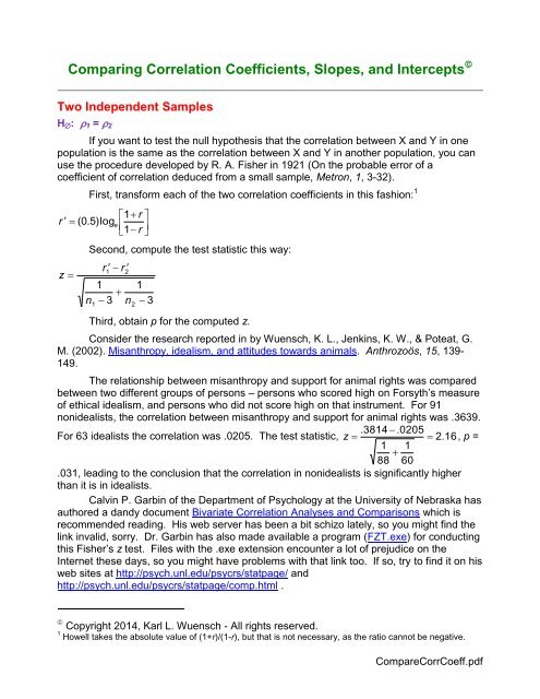
<strong>Comparing</strong> <strong>Correlation</strong> <strong>Coefficients</strong>, <strong>Slopes</strong>, <strong>and</strong> <strong>Intercepts</strong> <br />
Two Independent Samples<br />
H : 1 = 2<br />
If you want to test the null hypothesis that the correlation between X <strong>and</strong> Y in one<br />
population is the same as the correlation between X <strong>and</strong> Y in another population, you can<br />
use the procedure developed by R. A. Fisher in 1921 (On the probable error of a<br />
coefficient of correlation deduced from a small sample, Metron, 1, 3-32).<br />
First, transform each of the two correlation coefficients in this fashion: 1<br />
1<br />
r<br />
r ( 0.5)log<br />
e <br />
1<br />
r<br />
z <br />
<br />
<br />
<br />
Second, compute the test statistic this way:<br />
1<br />
r r <br />
1<br />
2<br />
1<br />
<br />
n 3 n<br />
2<br />
1<br />
3<br />
Third, obtain p for the computed z.<br />
Consider the research reported in by Wuensch, K. L., Jenkins, K. W., & Poteat, G.<br />
M. (2002). Misanthropy, idealism, <strong>and</strong> attitudes towards animals. Anthrozoös, 15, 139-<br />
149.<br />
The relationship between misanthropy <strong>and</strong> support for animal rights was compared<br />
between two different groups of persons – persons who scored high on Forsyth’s measure<br />
of ethical idealism, <strong>and</strong> persons who did not score high on that instrument. For 91<br />
nonidealists, the correlation between misanthropy <strong>and</strong> support for animal rights was .3639.<br />
.3814 .0205<br />
For 63 idealists the correlation was .0205. The test statistic, z <br />
2. 16, p =<br />
1 1<br />
<br />
88 60<br />
.031, leading to the conclusion that the correlation in nonidealists is significantly higher<br />
than it is in idealists.<br />
Calvin P. Garbin of the Department of Psychology at the University of Nebraska has<br />
authored a d<strong>and</strong>y document Bivariate <strong>Correlation</strong> Analyses <strong>and</strong> Comparisons which is<br />
recommended reading. His web server has been a bit schizo lately, so you might find the<br />
link invalid, sorry. Dr. Garbin has also made available a program (FZT.exe) for conducting<br />
this Fisher’s z test. Files with the .exe extension encounter a lot of prejudice on the<br />
Internet these days, so you might have problems with that link too. If so, try to find it on his<br />
web sites at http://psych.unl.edu/psycrs/statpage/ <strong>and</strong><br />
http://psych.unl.edu/psycrs/statpage/comp.html .<br />
Copyright 2014, Karl L. Wuensch - All rights reserved.<br />
1 Howell takes the absolute value of (1+r)/(1-r), but that is not necessary, as the ratio cannot be negative.<br />
CompareCorrCoeff.pdf
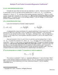
If you are going to compare correlation coefficients, you should also compare<br />
slopes. It is quite possible for the slope for predicting Y from X to be different in one<br />
population than in another while the correlation between X <strong>and</strong> Y is identical in the two<br />
populations, <strong>and</strong> it is also quite possible for the correlation between X <strong>and</strong> Y to be different<br />
in one population than in the other while the slopes are identical, as illustrated below:<br />
2<br />
On the left, we can see that the slope is the same for the relationship plotted with<br />
blue o’s <strong>and</strong> that plotted with red x’s, but there is more error in prediction (a smaller<br />
Pearson r ) with the blue o’s. For the blue data, the effect of extraneous variables on the<br />
predicted variable is greater than it is with the red data.<br />
On the right, we can see that the slope is clearly higher with the red x’s than with<br />
the blue o’s, but the Pearson r is about the same for both sets of data. We can predict<br />
equally well in both groups, but the Y variable increases much more rapidly with the X<br />
variable in the red group than in the blue.<br />
H : b 1 = b 2<br />
Let us test the null hypothesis that the slope for predicting support for animal rights<br />
from misanthropy is the same in nonidealists as it is in idealists.<br />
First we conduct the two regression analyses, one using the data from nonidealists,<br />
the other using the data from the idealists. Here are the basic statistics:<br />
Group Intercept Slope SE slope SSE SD X n<br />
Nonidealists 1.626 .3001 .08140 24.0554 .6732 91<br />
Idealists 2.404 .0153 .09594 15.6841 .6712 63<br />
The test statistic is Student’s t, computed as the difference between the two slopes<br />
b1<br />
b2<br />
divided by the st<strong>and</strong>ard error of the difference between the slopes, that is, t on<br />
(N – 4) degrees of freedom.<br />
s b b<br />
1<br />
2
If your regression program gives you the st<strong>and</strong>ard error of the slope (both SAS <strong>and</strong><br />
SPSS do), the st<strong>and</strong>ard error of the difference between the two slopes is most easily<br />
2 2<br />
2<br />
2<br />
computed as s s s .08140 .09594 . 1258<br />
b1 b<br />
<br />
2 b1<br />
b2<br />
Or, if you just love doing arithmetic, you can first find the pooled residual variance,<br />
SSE1<br />
SSE<br />
<br />
n n 4<br />
24.0554<br />
15.6841<br />
<br />
150<br />
2<br />
2<br />
s y . x<br />
.2649,<br />
1 2<br />
<strong>and</strong> then compute the st<strong>and</strong>ard error of the difference between slopes as<br />
s<br />
2<br />
y.<br />
x<br />
SS<br />
X<br />
1<br />
above.<br />
s<br />
<br />
SS<br />
2<br />
y.<br />
x<br />
X<br />
2<br />
<br />
.2649<br />
(90).6732<br />
2<br />
.2649<br />
<br />
(62).6712<br />
2<br />
.1264, within rounding error of what we got<br />
.3001<br />
.0153<br />
Now we can compute the test statistic: t <br />
2. 26.<br />
.1258<br />
This is significant on 150 df (p = .025), so we conclude that the slope in nonidealists<br />
is significantly higher than that in idealists.<br />
Please note that the test on slopes uses a pooled error term. If the variance in the<br />
dependent variable is much greater in one group than in the other, there are alternative<br />
methods. See Kleinbaum <strong>and</strong> Kupper (1978, Applied Regression Analysis <strong>and</strong> Other<br />
Multivariable Methods, Boston: Duxbury, pages 101 & 102) for a large (each sample<br />
n > 25) samples test, <strong>and</strong> K & K page 192 for a reference on other alternatives to pooling.<br />
H : a 1 = a 2<br />
The regression lines (one for nonidealists, the other for idealists) for predicting<br />
support for animal rights from misanthropy could also differ in intercepts. Here is how to<br />
test the null hypothesis that the intercepts are identical:<br />
s<br />
t<br />
1<br />
<br />
n1<br />
n<br />
<br />
<br />
1<br />
2 2<br />
a<br />
pooled<br />
1 a<br />
s<br />
2<br />
y.<br />
x<br />
2<br />
a<br />
a<br />
1<br />
2<br />
M<br />
<br />
SS<br />
2<br />
1<br />
X1<br />
1 2<br />
df n1 n2<br />
4<br />
s a a<br />
M<br />
<br />
SS<br />
2<br />
2<br />
X 2<br />
<br />
<br />
<br />
M 1 <strong>and</strong> M 2 are the means on the predictor variable for the two groups (nonidealists <strong>and</strong><br />
idealists). If you ever need a large sample test that does not require homogeneity of<br />
variance, see K & K pages 104 <strong>and</strong> 105.<br />
s<br />
For our data,<br />
2<br />
1 1 2.3758<br />
2649<br />
<br />
91 63 (90).6732<br />
2<br />
2.2413<br />
<br />
(62).6712<br />
. a1a<br />
<br />
<br />
2<br />
2<br />
2<br />
<br />
<br />
<br />
.3024, <strong>and</strong><br />
1.626 2.404<br />
t <br />
2.57. On 150 df, p = .011. The intercept in idealists is<br />
.3024<br />
significantly higher than in nonidealists.<br />
3
4<br />
Potthoff Analysis<br />
A more sophisticated way to test these hypotheses would be to create K-1<br />
dichotomous “dummy variables” to code the K samples <strong>and</strong> use those dummy variables<br />
<strong>and</strong> the interactions between those dummy variables <strong>and</strong> our predictor(s) as independent<br />
variables in a multiple regression. For our problem, we would need only one dummy<br />
variable (since K = 2), the dichotomous variable coding level of idealism. Our predictors<br />
would then be idealism, misanthropy, <strong>and</strong> idealism x misanthropy (an interaction term).<br />
Complete details on this method (also known as the Potthoff method) are in Chapter 13 of<br />
K & K. We shall do this type of analysis when we cover multiple regression in detail in a<br />
subsequent course. If you just cannot wait until then, see my document <strong>Comparing</strong><br />
Regression Lines From Independent Samples .<br />
Correlated Samples<br />
H : WX = WY<br />
If you wish to compare the correlation between one pair of variables with that<br />
between a second, overlapping pair of variables (for example, when comparing the<br />
correlation between one IQ test <strong>and</strong> grades with the correlation between a second IQ test<br />
<strong>and</strong> grades), you can use Williams’ procedure explained in our textbook -- pages 261-262<br />
of Howell, D. C. (2007), Statistical Methods for Psychology, 6 th edition, Thomson<br />
Wadsworth. It is assumed that the correlations for both pairs of variables have been<br />
computed on the same set of subjects. The traditional test done to compare overlapping<br />
correlated correlation coefficients was proposed by Hotelling in 1940, <strong>and</strong> is still often<br />
used, but it has problems. Please see the following article for more details, including an<br />
alternate procedure that is said to be superior to Williams’ procedure: Meng, Rosenthal, &<br />
Rubin (1992) <strong>Comparing</strong> correlated correlation coefficients. Psychological Bulletin, 111:<br />
172-175. Also see the pdf document Bivariate <strong>Correlation</strong> Analyses <strong>and</strong> Comparisons<br />
authored by Calvin P. Garbin of the Department of Psychology at the University of<br />
Nebraska. Dr. Garbin has also made available a program for conducting (FZT.exe) for<br />
conducting such tests. It will compute both Hotelling’s t <strong>and</strong> the test recommended by<br />
Meng et al., Steiger’s Z. See my example, Steiger’s Z: Testing H : ay = by<br />
H : WX = YZ<br />
If you wish to compare the correlation between one pair of variables with that<br />
between a second (nonoverlapping) pair of variables, read the article by T. E.<br />
Raghunathan , R. Rosenthal, <strong>and</strong> D. B. Rubin (<strong>Comparing</strong> correlated but nonoverlapping<br />
correlations, Psychological Methods, 1996, 1, 178-183). Also, see my example,<br />
<strong>Comparing</strong> Correlated but Nonoverlapping <strong>Correlation</strong> <strong>Coefficients</strong><br />
SAS <strong>and</strong> SPSS code to conduct these analyses <strong>and</strong> more<br />
Return to my Statistics Lessons page.<br />
Copyright 2014, Karl L. Wuensch - All rights reserved.