The acoustics of public squares/places: a comparison ... - Odeon
The acoustics of public squares/places: a comparison ... - Odeon
The acoustics of public squares/places: a comparison ... - Odeon

You also want an ePaper? Increase the reach of your titles
YUMPU automatically turns print PDFs into web optimized ePapers that Google loves.
<strong>The</strong> 33 rd International Congress and Exposition<br />
on Noise Control Engineering<br />
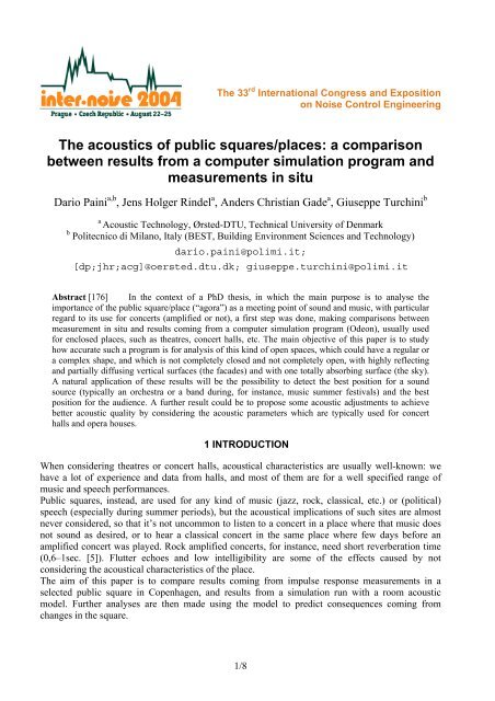
<strong>The</strong> <strong>acoustics</strong> <strong>of</strong> <strong>public</strong> <strong>squares</strong>/<strong>places</strong>: a <strong>comparison</strong><br />
between results from a computer simulation program and<br />
measurements in situ<br />
Dario Paini a,b , Jens Holger Rindel a , Anders Christian Gade a , Giuseppe Turchini b<br />
a Acoustic Technology, Ørsted-DTU, Technical University <strong>of</strong> Denmark<br />
b Politecnico di Milano, Italy (BEST, Building Environment Sciences and Technology)<br />
dario.paini@polimi.it;<br />
[dp;jhr;acg]@oersted.dtu.dk; giuseppe.turchini@polimi.it<br />
Abstract [176] In the context <strong>of</strong> a PhD thesis, in which the main purpose is to analyse the<br />
importance <strong>of</strong> the <strong>public</strong> square/place (“agora”) as a meeting point <strong>of</strong> sound and music, with particular<br />
regard to its use for concerts (amplified or not), a first step was done, making <strong>comparison</strong>s between<br />
measurement in situ and results coming from a computer simulation program (<strong>Odeon</strong>), usually used<br />
for enclosed <strong>places</strong>, such as theatres, concert halls, etc. <strong>The</strong> main objective <strong>of</strong> this paper is to study<br />
how accurate such a program is for analysis <strong>of</strong> this kind <strong>of</strong> open spaces, which could have a regular or<br />
a complex shape, and which is not completely closed and not completely open, with highly reflecting<br />
and partially diffusing vertical surfaces (the facades) and with one totally absorbing surface (the sky).<br />
A natural application <strong>of</strong> these results will be the possibility to detect the best position for a sound<br />
source (typically an orchestra or a band during, for instance, music summer festivals) and the best<br />
position for the audience. A further result could be to propose some acoustic adjustments to achieve<br />
better acoustic quality by considering the acoustic parameters which are typically used for concert<br />
halls and opera houses.<br />
1 INTRODUCTION<br />
When considering theatres or concert halls, acoustical characteristics are usually well-known: we<br />
have a lot <strong>of</strong> experience and data from halls, and most <strong>of</strong> them are for a well specified range <strong>of</strong><br />
music and speech performances.<br />
Public <strong>squares</strong>, instead, are used for any kind <strong>of</strong> music (jazz, rock, classical, etc.) or (political)<br />
speech (especially during summer periods), but the acoustical implications <strong>of</strong> such sites are almost<br />
never considered, so that it’s not uncommon to listen to a concert in a place where that music does<br />
not sound as desired, or to hear a classical concert in the same place where few days before an<br />
amplified concert was played. Rock amplified concerts, for instance, need short reverberation time<br />
(0,6–1sec. [5]). Flutter echoes and low intelligibility are some <strong>of</strong> the effects caused by not<br />
considering the acoustical characteristics <strong>of</strong> the place.<br />
<strong>The</strong> aim <strong>of</strong> this paper is to compare results coming from impulse response measurements in a<br />
selected <strong>public</strong> square in Copenhagen, and results from a simulation run with a room acoustic<br />
model. Further analyses are then made using the model to predict consequences coming from<br />
changes in the square.<br />
1/8
1.1 Choice <strong>of</strong> the Public Square for the measurements<br />
Different parameters were considered in order to choose the square which had the better<br />
characteristics for the measurements: shape <strong>of</strong> the square, dimensions, materials <strong>of</strong> the façades/<br />
floor, presence (or not) <strong>of</strong> lateral streets, height <strong>of</strong> the façades, presence (or not) <strong>of</strong> vegetation, habit<br />
to play concerts inside the square during summertime, etc. In order to have better results,<br />
measurements should have to be held within an acceptable (low) background noise level. It was<br />
soon clear that this was the main problem in a lot <strong>of</strong> <strong>public</strong> <strong>squares</strong>: noise from traffic, works in<br />
progress, many tourists passing by and talking, fountains, alarms, church bells, birds singing, etc.<br />
Finally a solution was found with the internal square <strong>of</strong> the Industrial Design Museum in<br />
Copenhagen (Kunst Industri Museet – Grønnegården). <strong>The</strong> Leq (A) <strong>of</strong> the background noise was 48<br />
dBA (see Figure 1). <strong>The</strong> only noises were from birds (above 4-8 kHz), some works in progress from<br />
a street close to the square (only during certain periods <strong>of</strong> the day), and some traffic noise (at low<br />
frequencies). <strong>The</strong> SNR was acceptable at almost all the frequency bands, even if with some<br />
problems at low frequencies (see further).<br />
<strong>The</strong> place is a rectangular shaped area <strong>of</strong> 84x60m; the height <strong>of</strong> the façades vary from 4.1m to<br />
9.2m (see Figure 2). <strong>The</strong> ro<strong>of</strong> is sloping with an angle <strong>of</strong> 39°; the irregular surface can cause a<br />
scattering effect especially at high frequencies. <strong>The</strong> “floor” is basically made <strong>of</strong> grass. Trees are<br />
distributed in a regular way in the square.<br />
80<br />
70<br />
60<br />
50<br />
40<br />
30<br />
20<br />
10<br />
0<br />
Background noise<br />
31,5 63 125 250 500 1000 2000 4000 8000 Leq(L) Leq(A)<br />
Lin A-w eight<br />
Figure 1 – Background noise during the measurements<br />
2 MEASUREMENTS<br />
Measurements were done during a cloudy day: temperature was 10°C, relative humidity at 70-80%,<br />
wind speed 3-4 m/s.<br />
2.1 Choice <strong>of</strong> the position <strong>of</strong> the sound source and receivers<br />
<strong>The</strong> sound source is represented by an omnidirectional dodecahedron loudspeaker (height = 1.5m),<br />
which was positioned in two points in the square, in an area where usually the orchestra is located<br />
during the concerts. <strong>The</strong> lower limit <strong>of</strong> the loudspeaker was 125Hz, which yielded to not consider<br />
the measurement down to this frequency band. <strong>The</strong> trees mainly form two double rows (see Figure<br />
3) distributed parallel to the lateral façades at 13-16m, so that the audience can just take place in the<br />
central part <strong>of</strong> the square: only the central area was considered for selecting the 7 receivers positions<br />
(omnidirectional microphone, height =1.3m); the chosen positions can be seen in the Figure 3.<br />
<strong>The</strong> s<strong>of</strong>tware “Dirac” was used, with an e-sweep <strong>of</strong> 10.9sec. In principle a larger length would have<br />
been used to increase the accuracy <strong>of</strong> the measurement, but the longer the signal, the higher the<br />
possibility <strong>of</strong> encountering external noises (such as airplanes, birds, church bells): 10.9 sec. seemed<br />
to be a good compromise.<br />
2/8
<strong>The</strong> following <strong>acoustics</strong> parameters were measured: reverberation parameters (EDT, T10, T20, and<br />
T30), energy ratios (C80, D50), and intelligibility parameters (STI male/female).<br />
Figure 2 – Kunst Industri Museet – Grønnegården<br />
3 SIMULATION WITH ODEON<br />
ODEON is PC s<strong>of</strong>tware used for simulation <strong>of</strong> interior <strong>acoustics</strong> <strong>of</strong> buildings. It uses prediction<br />
algorithms based on image-source method combined with ray tracing. and it’s usually used for the<br />
prediction <strong>of</strong> <strong>acoustics</strong> in large rooms such as concert halls, opera halls, auditoria, etc.<br />
3.1 Choice <strong>of</strong> the materials<br />
<strong>The</strong> choice <strong>of</strong> the materials is very important in order to have accurate results to be compared with<br />
measurements. It had rained before the measurement so that we had to take into account on this<br />
variation on <strong>Odeon</strong> simulation when selecting the appropriate absorbing coefficients.<br />
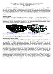
<strong>The</strong> façades are made basically <strong>of</strong> concrete walls and windows (glass and wooden frames). <strong>The</strong><br />
surface represented by windows (glass and wooden frame) was about 25% <strong>of</strong> the total. In order to<br />
have faster calculation without decreasing the quality <strong>of</strong> results, it seemed convenient to treat all the<br />
façades as unique mixed material made <strong>of</strong> the weighted contribution <strong>of</strong> each one (75%: concrete,<br />
21,25%: glass, 3,75%: solid wood). Scattering effects coming from the irregularities <strong>of</strong> the original<br />
surface were taken into account, adding a scattering coefficient <strong>of</strong> 0,1 in the calculation model. A<br />
higher scattering index (0,7) was added to the ro<strong>of</strong> <strong>of</strong> the buildings, due to its irregularities: this is<br />
good especially at mid-high frequencies. To calculate the absorbing coefficient <strong>of</strong> the grass the<br />
Delany and Bazley model was used, with a porosity σ = 100 kNsm -4 , to take into account the<br />
decreased porosity <strong>of</strong> the terrain due to the rain <strong>of</strong> the night before.<br />
7<br />
6 4 2<br />
5<br />
3<br />
1<br />
P1 1<br />
(a) -2004 (b)<br />
Figure 3 (a) & (b) – (a) <strong>The</strong> model as drawn with <strong>Odeon</strong>. It’s possible to see the source and receivers’<br />
positions, the distribution <strong>of</strong> the trees in the square etc. A black box surrounds the square: it a totally<br />
absorbing box which permits to have a completely closed volume. <strong>The</strong> upper face <strong>of</strong> the box is <strong>of</strong> course<br />
modeling the sky as well. (b) Overview <strong>of</strong> the modeled <strong>public</strong> square<br />
3/8
<strong>The</strong> trees were modelled like a cylinder (the trunk), high reflecting at high and low frequencies,<br />
which a scattering index <strong>of</strong> 0,7, and two circles (perpendicular one to each other) which represent<br />
the beams. To get a more realistic behaviour <strong>of</strong> the model, they are considered 50% transparent with<br />
a scattering <strong>of</strong> 0,6. <strong>The</strong> “ceiling” <strong>of</strong> the square is represented by the sky which is totally absorbing<br />
at all frequencies.<br />
A <strong>comparison</strong> among different <strong>acoustics</strong> parameters, usually used in evaluating the <strong>acoustics</strong> <strong>of</strong><br />
theatres and concert halls, was done.<br />
In order to compare simulation with the measured results, the error was defined as [2]:<br />
APmeasured<br />
− APsimulated<br />
Error = (1)<br />
SL<br />
where:<br />
is the measured value <strong>of</strong> the current <strong>acoustics</strong> parameter<br />
APmeasured<br />
APsimulated<br />
is the simulated value <strong>of</strong> the current acoustic parameter<br />
SL is a subjective limen for the current acoustic parameter (ex.: SL for T30 is 5% <strong>of</strong> the<br />
measured value [1])<br />
<strong>The</strong> error is calculated for 4 classes <strong>of</strong> simulation, for each receiver point:<br />
- 180.000 rays; TO 1 = 2<br />
- 300.000 rays, TO = 1<br />
- 300.000 rays – TO = 2<br />
- 300.000 rays – TO = 2, with low scattering index (=0,2) on the ro<strong>of</strong> <strong>of</strong> the building<br />
- 500.000 rays – TO = 2, with low scattering index (=0,2) on the ro<strong>of</strong> <strong>of</strong> the building<br />
Low TO seems to increase the error. Using 180.000 rays (TO=2) gave the minimum errors at midhigh<br />
frequency band, while at low frequencies 300k or 500k rays (with low scattering <strong>of</strong> the ro<strong>of</strong>)<br />
seem to be better, as shown in the next figure from R5). For further analysis, data from 180.000 rays<br />
(TO=2) will be used.<br />
18<br />
16<br />
14<br />
12<br />
10<br />
8<br />
6<br />
4<br />
2<br />
0<br />
[S1R5] T30 Error<br />
180k rays - TO2<br />
300k rays - TO1<br />
300k rays - TO2<br />
300k rays - TO2 - low scatt<br />
500k rays - TO2 - low scatt<br />
125 250 500 1000 2000 4000 8000<br />
Figure 4 – T30 - Comparison <strong>of</strong> error in SL-units, with different calculation parameters<br />
<strong>The</strong> first parameter that was compared was reverberation time (T30), which can be considered one<br />
<strong>of</strong> the main factors “governing most aspects <strong>of</strong> overall room <strong>acoustics</strong> as heard by the audience” [3].<br />
As reverberation time is not usually position dependant, average and standard deviation from each<br />
receiver point were calculated (for each frequency band), both for the measured and for the<br />
simulated values. Results (Figure 5) state that the accuracy <strong>of</strong> the simulation is good if compared<br />
with the measured averaged values; low values <strong>of</strong> standard deviation from 250 up to 8k Hz mean<br />
that there aren’t great variations <strong>of</strong> T30 among the receivers’ positions. <strong>The</strong> quite high value <strong>of</strong><br />
1 Below the transition order, calculations are carried out using the "Image Source Method", above the transition a<br />
special ray-tracing algorithm is used (from <strong>Odeon</strong> Manual)<br />
4/8
standard deviation at 125Hz, for measured data can be attributed to low SNR during measurements<br />
(see par. 1.1).<br />
[s]<br />
2,50<br />
2,00<br />
1,50<br />
1,00<br />
0,50<br />
0,00<br />
T30: average and standard deviation:<br />
<strong>comparison</strong> between measured and calculated data<br />
125 250 500 1000 2000 4000 8000<br />
[Hz]<br />
1,00<br />
0,80<br />
0,60<br />
0,40<br />
0,20<br />
0,00<br />
T30_meas_aver T30_sim_aver std-dev_meas std-dev_sim<br />
Figure 5 – T30: <strong>comparison</strong> between the simulated and the measured data <strong>of</strong> average and standard deviation<br />
Clarity index C80 and Definition D50 are not so much frequency dependant, while they rather vary<br />
with the distance <strong>of</strong> the receiver from the source; for this reason average was calculated as:<br />
1<br />
AP =<br />
⋅∑<br />
( AP)<br />
f f<br />
# <strong>of</strong> freq. bands<br />
where AP stands for the acoustic parameter (C80 and D50), f is the frequency band considered (250 -<br />
2kHz).<br />
14,00<br />
12,00<br />
10,00<br />
8,00<br />
6,00<br />
4,00<br />
2,00<br />
0,00<br />
C80 - average and standard deviation:<br />
<strong>comparison</strong> between measured and calculated data<br />
S1R1 S1R2 S1R3 S1R4 S1R5 S1R6 S1R7<br />
[receiver pos.]<br />
C80_meas_aver C80_sim_aver<br />
C80_meas_std-dev C80_sim_std-dev<br />
(a)<br />
(b)<br />
Figure 6 – (a) ‘C80’ – (b) ‘D50’: <strong>comparison</strong> between the simulated and the measured data at different receiver<br />
points, <strong>of</strong> average and standard deviation (frequency range: 250-2kHz, octave band)<br />
1,00<br />
0,90<br />
0,80<br />
0,70<br />
0,60<br />
0,50<br />
0,40<br />
0,30<br />
0,20<br />
0,10<br />
0,00<br />
[std-dev]<br />
D50 - average and standard deviation:<br />
<strong>comparison</strong> between measured and calculated data<br />
S1R1 S1R2 S1R3 S1R4 S1R5 S1R6 S1R7<br />
[receiver pos.]<br />
D50_meas_aver D50_sim_aver<br />
D50_meas_std-dev D50_sim_std-dev<br />
S1R1 S1R2 S1R3 S1R4 S1R5 S1R6 S1R7<br />
8,0 12,0 18,0 20,1 28,0 29,4 38,0<br />
Table 1– Distances, in meters, from the source (S1) to the receivers (Rn)<br />
For both indexes the simulated values and the measured ones don’t fit so much at distances very<br />
closed to the source (S1R1-R2). In any case it’s interesting to consider the decreasing <strong>of</strong> C80 and<br />
D50 with distance from the source.<br />
<strong>The</strong> STI (Speech Intelligibility Index) was compared, as well, giving very good results at each<br />
receiver point, as shown in Figure 7, from which it’s interesting to see the decreasing <strong>of</strong> STI as a<br />
function <strong>of</strong> the distance from the source. <strong>The</strong> critical distance 2 was calculated to be approximately<br />
14,4m (at 2kHz), which means that below this distance the direct sound is higher than the<br />
2 <strong>The</strong> “critical distance” is defined as the distance from the sound source at which the direct and reflected sound<br />
energies are equal. Above this distance the overall sound pressure level is constant in the room in the form <strong>of</strong> a "diffuse<br />
sound field". A very reverberant room has a short critical distance.<br />
5/8<br />
(2)
everberant one (which is the case <strong>of</strong> receivers R1 and R2), with respect <strong>of</strong> source position S1:<br />
STIR1 and STIR2 are very high for that reason, and above the critical path (R3 to R7) the acoustic <strong>of</strong><br />
the square affects the speech intelligibility index. STI is affected by RT and background noise.<br />
During the simulation no background noise was added, and usually, during a measurement the SNR<br />
is to be acceptable to have good accuracy. During our measurement, anyway, some non-stationary<br />
noises (like airplanes, birds, etc.) were present during some <strong>of</strong> the measurements. This is why the<br />
STI simulated by <strong>Odeon</strong> is almost always higher than the one measured by Dirac.<br />
STI Odw<br />
STI meas -<br />
female<br />
STI meas -<br />
male<br />
1<br />
0,8<br />
0,6<br />
0,4<br />
0,2<br />
0<br />
STI<br />
S1R1 S1R2 S1R3 S1R4 S1R5 S1R6 S1R7<br />
STI Odw 0,89 0,84 0,79 0,70 0,69 0,69 0,59<br />
STI meas - female 0,82 0,88 0,71 0,72 0,66 0,65 0,52<br />
STI meas - male 0,80 0,87 0,70 0,71 0,66 0,64 0,52<br />
Figure 7 – STI <strong>comparison</strong> between the simulated and the measured data at each receiver position. <strong>The</strong><br />
receivers on the left <strong>of</strong> the red dashed line are positioned within the critical distance, while the ones on the<br />
right are positioned beyond it.<br />
4 FURTHER ANALYSIS<br />
As all the simulated acoustic parameters are fitting well (especially at mid-high frequencies) if<br />
compared with the measured ones, some further analysis can be done.<br />
4.1 Auralisation<br />
Auralisation was done in order to hear the effect <strong>of</strong> the square with different kinds <strong>of</strong> music.<br />
Different sample were considered: for classical music, if not amplified, the main problem is the<br />
propagation <strong>of</strong> sound toward the rear part <strong>of</strong> the audience, as no reflectors are present. On the other<br />
hand the main problem for speech and amplified rock or jazz concerts is represented by flutter<br />
echoes, perceivable also just clapping hands in the “real” site.<br />
4.2 Analysis <strong>of</strong> the impulse response with and without trees<br />
To analyze the importance <strong>of</strong> trees in scattering sound, and so avoiding some effects <strong>of</strong> flutter<br />
echoes, or to increase the clarity C80 and the speech transmission index, a new simulation was done<br />
taking away trees from the model, and looking at the impulse response (Figure 8-b).<br />
Reflections come mainly from frontal/rear and side façades. If they come from the wall in front <strong>of</strong><br />
the audience, then the angle <strong>of</strong> incidence is about 0°; for such a case the following formula can be<br />
used [4]:<br />
∆L ≈ −0,<br />
6 ⋅ t0<br />
− 8 [dB] (3)<br />
which gives the threshold <strong>of</strong> absolute perceptibility, and tells that if the delay (in milliseconds)<br />
between the direct and the first reflection is t0, then the reflected sound is still audible as a distinct<br />
sound (flutter echo) even when the difference Ldirect – Lreflected is ∆L.<br />
In both cases (a) and (b) the frontal reflection is heard at 0,318s, which means 143ms after the direct<br />
sound. This leads to ∆L=-93,8dB. In Figure 8 level are expressed in p(%): the direct and the<br />
6/8
eflected sound are respectively 100% and 21%, so that ∆L=10*Log(0,21 2 )=-13,5dB: this sound is<br />
perceived as a flutter echo.<br />
p (%)<br />
100<br />
80<br />
60<br />
40<br />
20<br />
0<br />
-20<br />
-40<br />
-60<br />
-80<br />
time (seconds)<br />
Right ear<br />
0,05 0,1 0,15 0,2 0,25 0,3 0,35 0,4 0,45 0,5 0,55 0,6 0,65 0,7 0,75 0,8 0,85 0,9 0,95 1<br />
<strong>Odeon</strong>©1985-2004<br />
time (seconds)<br />
(a)<br />
( )<br />
p (%)<br />
100<br />
80<br />
60<br />
40<br />
20<br />
0<br />
-20<br />
-40<br />
-60<br />
-80<br />
Right ear<br />
0,05 0,1 0,15 0,2 0,25 0,3 0,35 0,4 0,45 0,5 0,55 0,6 0,65 0,7 0,75 0,8 0,85 0,9 0,95 1<br />
<strong>Odeon</strong>©1985-2004<br />
time (seconds)<br />
(b)<br />
Figure 8 – Impulse response – [receiver position: R5] <strong>comparison</strong> between the impulse responses coming<br />
from the <strong>Odeon</strong> simulation, run with (a) and without (b) the trees. In (a), after the direct sound there are<br />
many weak reflections which come from the trees, which can improve clarity, D50 and STI. In (b), instead,<br />
after the direct sound, such reflections are hardly seen: a flutter echo is “added” at 0,291s.<br />
Same computation can be done for the case (b) “without trees”; the new reflection which is added at<br />
0,291s could be perceived as a flutter echo, for the same reason explained before.<br />
Putting more trees could be a solution in such a situation, to avoid flutter echoes.<br />
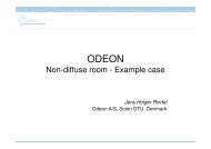
<strong>The</strong> same can be seen in Figure 9, which is a 3D-billiard simulation; it can be used for investigating<br />
or demonstrating effects such as scattering effects, flutter echoes or coupling effects. A number <strong>of</strong><br />
billiard balls are emitted from the source and reflected by the surfaces in the room.<br />
It can be demonstrated that trees can increase the level <strong>of</strong> C80, D50 and STI.<br />
0.00 10.00 20.00 30.00 40.00 50.00 60.00 70.00 80.00 metres<br />
Refl. order/ colou r:[0] [1] [2] [3] [4] [5] [>=6]<br />
<strong>Odeon</strong>©1985-2004<br />
P1<br />
Path : 39.80<br />
Time : 116<br />
Lost balls: 615<br />
Figure 9 – “3D-billiard simulation” - contributions <strong>of</strong> the trees (at mid-high frequency) on sound propagation<br />
from an omnidirectional source. Without the trees we shouldn’t have all the scattered sounds (isolated<br />
billiard balls in the centre <strong>of</strong> the square). Presence <strong>of</strong> trees can reduce the possibility <strong>of</strong> flutter echoes.<br />
Different colors mean different reflection orders.<br />
4.3 Lateral Energy Fraction<br />
Values <strong>of</strong> LEF, in large concert halls may vary between 0 and 0.5 [4]. This index can be calculated<br />
either by <strong>Odeon</strong> or by the formula:<br />
7/8
LEF = 0 , 39 − 0,<br />
0061⋅Width<br />
(4)<br />
Both <strong>Odeon</strong> and the formula give the value <strong>of</strong> about 0,024, especially at high distances from the<br />
source.<br />
4.4 Statistical Reverberation Time: a Quick Estimation<br />
When organizing a concert in a <strong>public</strong> square, a quick estimation <strong>of</strong> the RT could be useful to<br />
realize how the concert will sound.<br />
<strong>The</strong> calculation <strong>of</strong> error was done, taking into account the RT formula by Sabine, Eyring and Arau-<br />
Puchades. Despite the assumption for Sabine RT formulae is that the sound field is diffuse (all<br />
surfaces have the same absorption properties, no de-coupling effects, etc.) it came out that this is the<br />
most accurate, even if the error is quite large. Hence, a good way <strong>of</strong> calculating an accurate RT<br />
could be:<br />
RTsabine<br />
RT =<br />
sabine _ corr<br />
(5)<br />
where RTsabine_corr is the ‘real’ RT<br />
C=RTsabine/RTmeasured is a correction and, in our <strong>comparison</strong>s, it’s usually 0,7-0,8<br />
RTmeasured<br />
(RTsabine