A Short SVM (Support Vector Machine) Tutorial ... - JP Lewis

More documents

Recommendations

Info

This is also (somewhat) intuitive – if this were not the case (and the lagrangian was to be minimized wrt λ), subject to the previously stated constraint λ ≥ 0, then the ideal solution λ = 0 would remove the constraints entirely. Background: Optimization dual problem Optimization problems can be converted to their dual form by differentiating the Lagrangian wrt the original variables, solving the results so obtained for those variables if possible, and substituting the resulting expression(s) back into the Lagrangian, thereby eliminating the variables. The result is an equation in the lagrange multipliers, which must be maximized. Inequality constraints in the original variables also change to equality constraints in the multipliers. The dual form may or may not be simpler than the original (primal) optimization. In the case of SVMs, the dual form has simpler constraints, but the real reason for using the dual form is that it puts the problem in a form that allows the kernel trick to be used, as described below. The fact that the dual problem requires maximization wrt the multipliers carries over from the KKT condition. Conversion from the primal to the dual converts the problem from a saddle point to a simple maximum. A worked example, general quadratic with general linear constraint. α is the lagrange multiplier vector Lp = 1 x ′ Kx + c ′ x + α ′ (Ax + d) 2 dLp = Kx + c + A ′ α = 0 dx Kx = −A ′ α − c substitute this x into Lp: (assume K is symmetric) X ≡ K(−K −1 A ′ α − K −1 c) x = −K −1 A ′ α − K −1 c 1 (−K −1 A ′ α − K −1 c) ′ K(−K −1 A ′ α − K −1 c) − c ′ (K −1 A ′ α + K −1 c) + α ′ (A(−K −1 A ′ α − K −1 c) + d) 2 [ ] −( 1 α ′ AK −1 X) − ( 1 c ′ K −1 X) − c ′ K −1 A ′ α − c ′ K −1 c − α ′ AK −1 A ′ α − α ′ AK −1 c + α ′ d 2 2 [ ] = 1 (α ′ AK −1 KK −1 A ′ α + α ′ AK −1 KK −1 c) + (c ′ K −1 KK −1 A ′ α + c ′ K −1 KK −1 c) + · · · 2 = 1 α ′ AK −1 A ′ α + c ′ K −1 A ′ α + 1 c ′ K −1 c − c ′ K −1 c − c ′ K −1 A ′ α − α ′ AK −1 A ′ α − α ′ AK −1 c + α ′ d 2 2 = L d = − 1 α ′ AK −1 A ′ α − 1 c ′ K −1 c − α ′ AK −1 c + α ′ d 2 2 The − 1 2 c′ K −1 c can be ignored because it is a constant term wrt the independent variable α so the result is of the form − 1 2 α ′ Qα − α ′ Rc + α ′ d The constraints are now simply α ≥ 0. 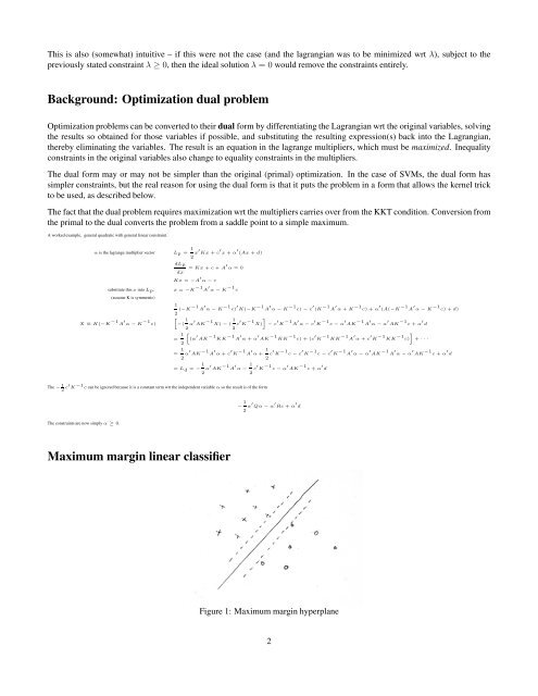Maximum margin linear classifier Figure 1: Maximum margin hyperplane 2
SVMs start from the goal of separating the data with a hyperplane, and extend this to non-linear decision boundaries using the kernel trick described below. The equation of a general hyperplane is w ′ x + b = 0 with x being the point (a vector), w the weights (also a vector). The hyperplane should separate the data, so that w ′ x k + b > 0 for all the x k of one class, and w ′ x j + b < 0 for all the x j of the other class. If the data are in fact separable in this way, there is probably more than one way to do it. Among the possible hyperplanes, SVMs select the one where the distance of the hyperplane from the closest data points (the “margin”) is as large as possible (Fig. 1). This sounds reasonable, and the resulting line in the 2D case is similar to the line I would probably pick to separate the classes. The Scholkopf/Smola book describes an intuitive justification for this criterion: suppose the training data are good, in the sense that every possible test vector is within some radius r of a training vector. Then, if the chosen hyperplane is at least r from any training vector it will correctly separate all the test data. By making the hyperplane as far as possible from any data, r is allowed to be correspondingly large. The desired hyperplane (that maximizes the margin) is also the bisector of the line between the closest points on the convex hulls of the two data sets. Now, find this hyperplane. By labeling the training points by y k ∈ −1, 1, with 1 being a positive example, −1 a negative training example, y k (w ′ x k + b) ≥ 0 for all points Both w, b can be scaled without changing the hyperplane. To remove this freedom, scale w, b so that y k (w ′ x k + b) ≥ 1 ∀k Next we want an expression for the distance between the hyperplane and the closest points; w, b will be chosen to maximize this expression. Imagine additional “supporting hyperplanes” (the dashed lines in Fig. 1) parallel to the separating hyperplane and passing through the closest points (the support points). These are y j (w ′ x j + b) = 1, y k (w ′ x k + b) = 1 for some points j, k (there may be more than one such point on each side). Figure 2: a - b = 2m The distance between the separating hyperplane and the nearest points (the margin) is half of the distance between these support hyperplanes, which is the same as the difference between the distances to the origin of the closest point on each of the support hyperplanes (Fig. 2). The distance of the closest point on a hyperplane to the origin can be found by minimizing x ′ x subject to x being on the hyperplane, minx ′ x + λ(w ′ x + b − 1) x d = 0 = 2x + λw = 0 dx → x = − λ 2 w 3
Page 1: A Short SVM (Support Vector Machine
Page 5 and 6: Reducing α allows more of the data

A Short SVM (Support Vector Machine) Tutorial ... - JP Lewis

You also want an ePaper? Increase the reach of your titles

Delete template?

Save as template?