Fast Normalized Cross-Correlation - JP Lewis

Abstract
This is an expanded version of a
paper from Vision Interface, 1995
(reference [10])
Fast Normalized Cross-Correlation
Although it is well known that cross correlation can be
efficiently implemented in the transform domain, the normalized
form of cross correlation preferred for feature
matching applications does not have a simple frequency
domain expression. Normalized cross correlation has
been computed in the spatial domain for this reason. This
short paper shows that unnormalized cross correlation
can be efficiently normalized using precomputing integrals
of the image and image 2 over the search window.
1 Introduction
The correlation between two signals (cross correlation) is
a standard approach to feature detection [6, 7] as well as
a component of more sophisticated techniques (e.g. [3]).
Textbook presentations of correlation describe the convolution
theorem and the attendant possibility of efficiently
computing correlation in the frequency domain using the
fast Fourier transform. Unfortunately the normalized
form of correlation (correlation coefficient) preferred in
template matching does not have a correspondingly simple
and efficient frequency domain expression. For this
reason normalized cross-correlation has been computed
in the spatial domain (e.g., [7], p. 585). Due to the computational
cost of spatial domain convolution, several inexact
but fast spatial domain matching methods have also
been developed [2]. This paper describes a recently introduced
algorithm [10] for obtaining normalized cross
correlation from transform domain convolution. The new
algorithm in some cases provides an order of magnitude
speedup over spatial domain computation of normalized
cross correlation (Section 5).
Since we are presenting a version of a familiar and
widely used algorithm no attempt will be made to survey
the literature on selection of features, whitening,
fast convolution techniques, extensions, alternate techniques,
or applications. The literature on these topics can
be approached through introductory texts and handbooks
∗ Current address: Interval Research, Palo Alto CA
zilla@computer.org
J. P. Lewis ∗
Industrial Light & Magic
[16, 7, 13] and recent papers such as [1, 19]. Nevertheless,
due to the variety of feature tracking schemes that
have been advocated it may be necessary to establish that
normalized cross-correlation remains a viable choice for
some if not all applications. This is done in section 3.
In order to make the paper self contained, section 2 describes
normalized cross-correlation and section 4 briefly
reviews transform domain and other fast convolution approaches
and the phase correlation technique. These sections
can be skipped by most readers. Section 5 describes
how normalized cross-correlation can be obtained from a
transform domain computation of correlation. Section 6
presents performance results.
2 Template Matching by Cross-
Correlation
The use of cross-correlation for template matching is motivated
by the distance measure (squared Euclidean distance)
�
(u, v) = [f(x, y) − t(x − u, y − v)] 2
d 2 f,t
x,y
(where f is the image and the sum is over x, y under the
window containing the feature t positioned at u, v). In
the expansion of d 2
d 2 f,t(u, v) = �
[f 2 (x, y) − 2f(x, y)t(x − u, y − v)
x,y
+ t 2 (x − u, y − v)]
the term � t2 �
(x − u, y − v) is constant. If the term
2 f (x, y) is approximately constant then the remaining
cross-correlation term
c(u, v) = �
f(x, y)t(x − u, y − v) (1)
x,y
is a measure of the similarity between the image and the
feature.
There are several disadvantages to using (1) for template
matching:

• If the image energy � f 2 (x, y) varies with position,
matching using (1) can fail. For example, the correlation
between the feature and an exactly matching
region in the image may be less than the correlation
between the feature and a bright spot.
• The range of c(u, v) is dependent on the size of the
feature.
• Eq. (1) is not invariant to changes in image amplitude
such as those caused by changing lighting conditions
across the image sequence.
The correlation coefficient overcomes these difficulties
by normalizing the image and feature vectors to unit
length, yielding a cosine-like correlation coefficient
γ(u, v) = (2)
�
x,y [f(x, y) − ¯ fu,v][t(x − u, y − v) − ¯t]
�� x,y [f(x, y) − ¯ �
fu,v]
2
x,y [t(x − u, y − v) − ¯t] 2
� 0.5
where ¯t is the mean of the feature and ¯ fu,v is the mean of
f(x, y) in the region under the feature. We refer to (2) as
normalized cross-correlation.
3 Feature Tracking Approaches
and Issues
It is clear that normalized cross-correlation (NCC) is not
the ideal approach to feature tracking since it is not invariant
with respect to imaging scale, rotation, and perspective
distortions. These limitations have been addressed in
various schemes including some that incorporate NCC as
a component. This paper does not advocate the choice
of NCC over alternate approaches. Rather, the following
discussion will point out some of the issues involved in
various approaches to feature tracking, and will conclude
that NCC is a reasonable choice for some applications.
SSDA. The basis of the sequential similarity detection algorithm
(SSDA) [2] is the observation that full precision
is only needed near the maximum of the cross-correlation
function, while reduced precision can be used elsewhere.
The authors of [2] describe several ways of implementing
‘reduced precision’. An SSDA implementation of crosscorrelation
proceeds by computing the summation in (1)
in random order and uses the partial computation as a
Monte Carlo estimate of whether the particular match location
will be near a maximum of the correlation surface.
The computation at a particular location is terminated before
completing the sum if the estimate suggests that the
location corresponds to a poor match.
The SSDA algorithm is simple and provides a significant
speedup over spatial domain cross-correlation. It
has the disadvantage that it does not guarantee finding
the maximum of the correlation surface. SSDA performs
well when the correlation surface has shallow slopes and
broad maxima. While this condition is probably satisfied
in many applications, it is evident that images containing
arrays of objects (pebbles, bricks, other textures) can generate
multiple narrow extrema in the correlation surface
and thus mislead an SSDA approach. A secondary disadvantage
of SSDA is that it has parameters that need to determined
(the number of terms used to form an estimate
of the correlation coefficient, and the early termination
threshold on this estimate).
Gradient Descent Search. If it is assumed that feature
translation between adjacent frames is small then the
translation (and parameters of an affine warp in [19]) can
be obtained by gradient descent [12]. Successful gradient
descent search requires that the interframe translation
be less than the radius of the basin surrounding the minimum
of the matching error surface. This condition may
be satisfied in many applications. Images sequences from
hand-held cameras can violate this requirement, however:
small rotations of the camera can cause large object translations.
Small or (as with SSDA) textured templates result
in matching error surfaces with narrow extrema and
thus constrain the range of interframe translation that can
be successfully tracked. Another drawback of gradient
descent techniques is that the search is inherently serial,
whereas NCC permits parallel implementation.
Snakes. Snakes (active contour models) have the disadvantage
that they cannot track objects that do not have a
definable contour. Some “objects” do not have a clearly
defined boundary (whether due to intrinsic fuzzyness or
due to lighting conditions), but nevertheless have a characteristic
distribution of color that may be trackable via
cross-correlation. Active contour models address a more
general problem than that of simple template matching
in that they provide a representation of the deformed
contour over time. Cross-correlation can track objects
that deform over time, but with obvious and significant
qualifications that will not be discussed here. Crosscorrelation
can also easily track a feature that moves by a
significant fraction of its own size across frames, whereas
this amount of translation could put a snake outside of its
basin of convergence.
Wavelets and other multi-resolution schemes. Although
the existence of a useful convolution theorem
for wavelets is still a matter of discussion (e.g., [11];
in some schemes wavelet convolution is in fact implemented
using the Fourier convolution theorem), efficient
feature tracking can be implemented with wavelets and

other multi-resolution representations using a coarse-tofine
multi-resolution search. Multi-resolution techniques
require, however, that the images contain sufficient low
frequency information to guide the initial stages of the
search. As discussed in section 6, ideal features are sometimes
unavailable and one must resort to poorly defined
“features” that may have little low-frequency information,
such as a configuration of small spots on an otherwise
uniform surface.
Each of the approaches discussed above has been advocated
by various authors, but there are fewer comparisons
between approaches. Reference [19] derives an optimal
feature tracking scheme within the gradient search
framework, but the limitations of this framework are not
addressed. An empirical study of five template matching
algorithms in the presence of various image distortions
[4] found that NCC provides the best performance
in all image categories, although one of the cheaper algorithms
performs nearly as well for some types of distortion.
A general hierarchical framework for motion tracking
is discussed in [1]. A correlation based matching approach
is selected though gradient approaches are also
considered.
Despite the age of the NCC algorithm and the existence
of more recent techniques that address its various shortcomings,
it is probably fair to say that a suitable replacement
has not been universally recognized. NCC makes
few requirements on the image sequence and has no parameters
to be searched by the user. NCC can be used ‘as
is’ to provide simple feature tracking, or it can be used
as a component of a more sophisticated (possibly multiresolution)
matching scheme that may address scale and
rotation invariance, feature updating, and other issues.
The choice of the correlation coefficient over alternative
matching criteria such as the sum of absolute differences
has also been justified as maximum-likelihood estimation
[18]. We acknowledge NCC as a default choice in many
applications where feature tracking is not in itself a subject
of study, as well as an occasional building block in
vision and pattern recognition research (e.g. [3]). A fast
algorithm is therefore of interest.
4 Transform Domain Computation
Consider the numerator in (2) and assume that we have
images f ′ (x, y) ≡ f(x, y)− ¯ fu,v and t ′ (x, y) ≡ t(x, y)−
¯t in which the mean value has already been removed:
num
γ (u, v) = �
x,y
f ′ (x, y)t ′ (x − u, y − v) (3)
For a search window of size M 2 and a feature of size N 2
(3) requires approximately N 2 (M − N + 1) 2 additions
and N 2 (M − N + 1) 2 multiplications.
Eq. (3) is a convolution of the image with the reversed
feature t ′ (−x, −y) and can be computed by
F −1 {F(f ′ )F ∗ (t ′ )} (4)
where F is the Fourier transform. The complex conjugate
accomplishes reversal of the feature via the Fourier
transform property Ff ∗ (−x) = F ∗ (ω).
Implementations of the FFT algorithm generally require
that f ′ and t ′ be extended with zeros to a common
power of two. The complexity of the transform computation
(3) is then 12M 2 log2M real multiplications and
18M 2 log2M real additions/subtractions. When M is
much larger than N the complexity of the direct ‘spatial’
computation (3) is approximately N 2 M 2 multiplications/additions,
and the direct method is faster than the
transform method. The transform method becomes relatively
more efficient as N approaches M and with larger
M, N.
4.1 Fast Convolution
There are several well known “fast” convolution algorithms
that do not use transform domain computation
[13]. These approaches fall into two categories: algorithms
that trade multiplications for additional additions,
and approaches that find a lower point on the O(N 2 )
characteristic of (one-dimensional) convolution by embedding
sections of a one-dimensional convolution into
separate dimensions of a smaller multidimensional convolution.
While faster than direct convolution these algorithms
are nevertheless slower than transform domain
convolution at moderate sizes [13] and in any case they
do not address computation of the denominator of (2).
4.2 Phase Correlation
Because (4) can be efficiently computed in the transform
domain, several transform domain methods of approximating
the image energy normalization in (2) have been
developed. Variation in the image energy under the template
can be reduced by high-pass filtering the image before
cross-correlation. This filtering can be conveniently
added to the frequency domain processing, but selection
of the cutoff frequency is problematic—a low cutoff may
leave significant image energy variations, whereas a high
cutoff may remove information useful to the match.
A more robust approach is phase correlation [9]. In
this approach the transform coefficients are normalized
to unit magnitude prior to computing correlation in the
frequency domain. Thus, the correlation is based only
on phase information and is insensitive to changes in

image intensity. Although experience has shown this
approach to be successful, it has the drawback that all
transform components are weighted equally, whereas one
might expect that insignificant components should be
given less weight. In principle one should select the spectral
pre-filtering so as to maximize the expected correlation
signal-to-noise ratio given the expected second order
moments of the signal and signal noise. This approach is
discussed in [16] and is similar to the classical matched
filtering random signal processing technique. With typical
(ρ ≈ 0.95) image correlation the best pre-filtering is
approximately Laplacian rather than a pure whitening.
5 Normalizing
Examining again the numerator of (2), we note that the
mean of the feature can be precomputed, leaving
num
γ (u, v) = � f(x, y)t ′ (x − u, y − v)
− ¯ �
′
fu,v t (x − u, y − v)
Since t ′ �
has zero mean and thus zero sum the term
¯fu,v
′ t (x − u, y − v) is also zero, so the numerator of
the normalized cross-correlation can be computed using
(4).
Examining the denominator of (2), the length of the feature
vector can be precomputed in approximately 3N 2
operations (small compared to the cost of the crosscorrelation),
and in fact the feature can be pre-normalized
to length one.
The problematic quantities are those in the expression
�
x,y [f(x, y)− ¯ fu,v] 2 . The image mean and local (RMS)
energy must be computed at each u, v, i.e. at (M − N +
1) 2 locations, resulting in almost 3N 2 (M −N +1) 2 operations
(counting add, subtract, multiply as one operation
each). This computation is more than is required for the
direct computation of (3) and it may considerably outweight
the computation indicated by (4) when the transform
method is applicable. A more efficient means of
computing the image mean and energy under the feature
is desired.
These quantities can be efficiently computed from tables
containing the integral (running sum) of the image and
image square over the search area, i.e.,
s(u, v) = f(u, v)+s(u−1, v)+s(u, v−1)−s(u−1, v−1)
s 2 (u, v) = f 2 (u, v) + s 2 (u − 1, v)
+ s 2 (u, v − 1) − s 2 (u − 1, v − 1)
with s(u, v) = s 2 (u, v) = 0 when either u, v < 0. The
energy of the image under the feature positioned at u, v
is then
ef (u, v) = s 2 (u + N − 1, v + N − 1)
− s 2 (u − 1, v + N − 1)
− s 2 (u + N − 1, v − 1)
+ s 2 (u − 1, v − 1)
and similarly for the image sum under the feature.
The problematic quantity �
x,y [f(x, y) − ¯ fu,v] 2 can now
be computed with very few operations since it expands
into an expression involving only the image sum and sum
squared under the feature. The construction of the tables
requires approximately 3M 2 operations, which is
less than the cost of computing the numerator by (4) and
considerably less than the 3N 2 (M − N + 1) 2 required to
compute �
x,y [f(x, y) − ¯ fu,v] 2 at each u, v.
This technique of computing a definite sum from a precomputed
running sum has been independently used in
a number of fields; a computer graphics application is
developed in [5]. If the search for the maximum of the
correlation surface is done in a systematic row-scan order
it is possible to combine the table construction and
reference through state variables and so avoid explicitly
storing the table. When implemented on a general purpose
computer the size of the table is not a major consideration,
however, and flexibility in searching the correlation
surface can be advantageous. Note that the s(u, v)
and s 2 (u, v) expressions are marginally stable, meaning
that their z-transform H(z) = 1/(1 − z −1 ) (one dimensional
version here) has a pole at z = 1, whereas stability
requires poles to be strictly inside the unit circle [14].
The computation should thus use large integer rather than
floating point arithmetic.
6 Performance
The performance of this algorithm will be discussed in
the context of special effects image processing. The
integration of synthetic and processed images into special
effects sequences often requires accurate tracking
of sequence movement and features. The use of automated
feature tracking in special effects was pioneered
in movies such as Cliffhanger, Forest Gump, and Speed.
Recently cross-correlation based feature trackers have
been introduced in commercial image compositing systems
such as Flame/Flint [20], Matador, Advance [21],
and After Effects [22].
The algorithm described in this paper was developed for
the movie Forest Gump (1994), and has been used in a
number of subsequent projects. Special effects sequences
in that movie included the replacement of various moving
elements and the addition of a contemporary actor into

10
80
50
20
110
80
50
20
110
search window(s) length direct NCC fast NCC
168 × 86 896 frames 15 hours 1.7 hours
115 × 200, 150 × 150 490 frames 14.3 hours 57 minutes
Table 1: Two tracking sequences from Forest Gump were re-timed using both direct
and fast NCC algorithms using identical features and search windows on a 100 Mhz
R4000 processor. These times include a 16 2 sub-pixel search [17] at the location
of the best whole-pixel match. The sub-pixel search was computed using Eq. (2)
(direct convolution) in all cases.
feature size search window(s) Flint fast NCC
40 2 110 2 1 min. 40 seconds 16 seconds (subpixel=1)
40 2 110 2 n/a 21 seconds (subpixel=8)
Table 2: Measured tracking times on a short sequence using the commercial Flint
system and the algorithm described in the text. These are wall-clock times obtained
on an unloaded 200 Mhz R4400 processor with 380 megabytes of memory (no
swapping occurred). Flint settings were MATCH LUM(ONLY), FIXED REF, OVER-
SAMPLE OFF. It appears that subpixel search is only available in the more expensive
Flame system.
0
0.4 0.5 0.6 0.7 0.8 0.9
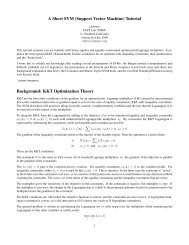
Figure 1: Measured relative performance of transform
domain versus spatial domain normalized crosscorrelation
as a function of the search window size (depth
axis) and the ratio of the feature size to search window
size.
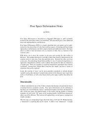
Figure 2: A tracked feature from a special effects sequence
in the movie Forest Gump. The region is out of
focus and has noticeable film-grain noise across frames.
A small (e.g. 10 2 or smaller) area from this region would
not provide a usable feature. The chosen feature size is
more than 40 2 pixels.

historical film and video sequences. Manually picked
features from one frame of a sequence were automatically
tracked over the remaining frames; this information
was used as the basis for further processing.
The relative performance of our algorithm is a function
of both the search window size and the ratio of the feature
size to search window size. Relative performance
increases along the window size axis (Fig. 1); a higher
resolution plot would show an additional ripple reflecting
the relation between the search window size and the
bounding power of two. The property that the relative
performance is greater on larger problems is desirable.
Table 1 illustrates the performance obtained in a special
effects feature tracking application. Table 2 compares
the performance of our algorithm with that of a high-end
commercial image compositing package.
Note that while a small (e.g. 10 2 ) feature size would suffice
in an ideal digital image, in practice much larger feature
sizes and search windows are sometimes required or
preferred:
• The image sequences used in film and video are
sometimes obtained from moving cameras and may
have considerable translation between frames due to
camera shake. Due to the high resolution required to
represent digital film, even a small movement across
frames may correspond to a distance of many pixels.
• The selected features are of course constrained to the
available features in the image; distinct “features”
are not always available at preferred scales and locations.
• Many potential features in a typical digitized image
are either out of focus or blurred due to motion of
the camera or object (Fig. 2). Feature match is also
hindered by imaging noise such as film grain. Large
features are more accurate in the presence of blur
and noise.
As a result of these considerations feature sizes of 20 2
and larger and search windows of 50 2 and larger are often
employed.
The fast algorithm in some cases reduces high-resolution
feature tracking from an overnight to an over-lunch procedure.
With lower (“proxy”) resolution and faster machines,
semi-automated feature tracking is tolerable in an
interactive system. Certain applications in other fields
may also benefit from the algorithm described here. 1
1 For example, image stabilization is a common feature in recent consumer
video cameras. Although most such systems are stabilized by
inertial means, one manufacturer implemented digital stabilization and
thus presumably used some form of image tracking. The algorithm used
leaves room for improvement however: it has been criticized as being
slow and unpredictable and a product review recommended leaving it
disabled [15].
References
[1] P. Anandan, “A Computational Framework and an
Algorithm for the Measurement of Visual Motion”,
Int. J. Computer Vision, 2(3), p. 283-310, 1989.
[2] D. I. Barnea, H. F. Silverman, “A class of algorithms
for fast digital image registration”, IEEE Trans. Computers,
21, pp. 179-186, 1972.
[3] R. Brunelli and T. Poggio, “Face Recognition: Features
versus Templates”, IEEE Trans. Pattern Analysis
and Machine Intelligence, vol. 15, no. 10,
pp. 1042-1052, 1993.
[4] P. J. Burt, C. Yen, X. Xu, “Local Correlation Measures
for Motion Analysis: a Comparitive Study”,
IEEE Conf. Pattern Recognition Image Processing
1982, pp. 269-274.
[5] F. Crow, “Summed-Area Tables for Texture Mapping”,
Computer Graphics, vol 18, No. 3, pp. 207-
212, 1984.
[6] R. O. Duda and P. E. Hart, Pattern Classification and
Scene Analysis, New York: Wiley, 1973.
[7] R. C. Gonzalez and R. E. Woods, Digital Image
Processing (third edition), Reading, Massachusetts:
Addison-Wesley, 1992.
[8] A. Goshtasby, S. H. Gage, and J. F. Bartholic, “A
Two-Stage Cross-Correlation Approach to Template
Matching”, IEEE Trans. Pattern Analysis and Machine
Intelligence, vol. 6, no. 3, pp. 374-378, 1984.
[9] C. Kuglin and D. Hines, “The Phase Correlation Image
Alignment Method,” Proc. Int. Conf. Cybernetics
and Society, 1975, pp. 163-165.
[10] J. P. Lewis, “Fast Template Matching”, Vision Interface,
p. 120-123, 1995.
[11] A. R. Lindsey, “The Non-Existence of a Wavelet
Function Admitting a Wavelet Transform Convolution
Theorem of the Fourier Type”, Rome Laboratory
Technical Report C3BB, 1995.
[12] B. D. Lucas and T. Kanade, “An Iterative Image
Registration Technique with an Application to Stereo
Vision”, IJCAI 1981.
[13] S. K. Mitra and J. F. Kaiser, Handbook for Digital
Signal Processing, New York: Wiley, 1993.
[14] A. V. Oppenheim and R. W. Schafer, Digital Signal
Processing, Englewood Cliffs, New Jersey: Prentice-
Hall, 1975.

[15] D. Polk, “Product Probe” – Panasonic PV-IQ604,
Videomaker, October 1994, pp. 55-57.
[16] W. Pratt, Digital Image Processing, John Wiley,
New York, 1978.
[17] Qi Tian and M. N. Huhns, “Algorithms for Subpixel
Registration”, CVGIP 35, p. 220-233, 1986.
[18] T. W. Ryan, “The Prediction of Cross-Correlation
Accuracy in Digital Stereo-Pair Images”, PhD thesis,
University of Arizona, 1981.
[19] J. Shi and C. Tomasi, “Good Features to Track”,
Proc. IEEE Conf. on Computer Vision and Pattern
Recognition, 1994.
[20] Flame effects compositing software, Discreet
Logic, Montreal, Quebec.
[21] Advance effects compositing software, Avid Technology,
Inc., Tewksbury, Massachusetts.
[22] After Effects effects compositing software, Adobe
(COSA), Mountain View, California.