A Short SVM (Support Vector Machine) Tutorial ... - JP Lewis

A Short SVM (Support Vector Machine) Tutorial
j.p.lewis
CGIT Lab / IMSC
U. Southern California
version 0.zz dec 2004
This tutorial assumes you are familiar with linear algebra and equality-constrained optimization/Lagrange multipliers. It explains
the more general KKT (Karush Kuhn Tucker) conditions for an optimum with inequality constraints, dual optimization,
and the “kernel trick”.
I wrote this to solidify my knowledge after reading several presentations of SVMs: the Burges tutorial (comprehensive and
difficult, probably not for beginners), the presentation in the Forsyth and Ponse computer vision book (easy and short, less
background explanation than here), the Cristianini and Shawe-Taylor SVM book, and the excellent Scholkopf/Smola Learning
with Kernels book.
’ means transpose.
Background: KKT Optimization Theory
KKT are the first-order conditions on the gradient for an optimal point. Lagrange multipliers (LM) extend the unconstrained
first-order condition (derivative or gradient equal to zero) to the case of equality constraints; KKT adds inequality constraints.
The SVM derivation will need two things from this section: complementarity condition and the fact that the Lagrangian is to
be maximized with respect to the multipliers.
To setup the KKT, form the Lagrangian by adding to the objective f(x) to be minimized equality and inequality constraints
(c k (x) = 0 or c k (x) ≥ 0) each with undetermined Lagrange-like multipliers λ k . By convention the KKT Lagrangian is
expressed by subtracting the constraints, while each lambda and constraint are positive:
L(x, λ) = f(x) − ∑ λ k c k (x) c k (x) ≥ 0, λ k ≥ 0
The gradient of the inequality constraints points to the interior of the feasible region. Then the optimum is a point where
These are the KKT conditions.
1) ∇f(x) − ∑ λ i ∇c i (x) = 0
2) λ i ≥ 0 and λ i c i (x) = 0 ∀i
The statement (1) is the same as what comes out of standard Lagrange multipliers, i.e. the gradient of the objective is parallel
to the gradient of the constraints.
The λ i c i (x) = 0 part is the complementarity condtion. For equality constraints, c k (x) = 0 so the condition holds. For
inequality constraints, either λ k = 0 or it must be that c k (x) = 0. This is intuitive: In the latter case the constraint is “active”,
in the former case the constraint is not zero, so it is inactive at this point (one can move a small distance in any direction without
violating the constraint). The active set is the union of the equality constraints and the inequality constraints that are active.
The multiplier gives the sensitivity of the objective to the constraints. If the constraint is inactive, the multiplier is zero. If
the multiplier is non-zero, the change in the Lagrangian due to a shift in the proposed optimum location is proportional to the
multiplier times the gradient of the constraint.
The KKT conditions are valid when the objective function is convex, and the constraints are also convex. A hyperplane (halfspace)
constraint is convex, as is the intersection of N convex sets (such as N hyperplane constraints).
The general problem is written as maximizing the Lagrangian wrt (= with respect to) the multipliers while minimizing the
Lagrangian wrt the other variables (a saddle point):
max
λ
min L(x; λ)
x
1

This is also (somewhat) intuitive – if this were not the case (and the lagrangian was to be minimized wrt λ), subject to the
previously stated constraint λ ≥ 0, then the ideal solution λ = 0 would remove the constraints entirely.
Background: Optimization dual problem
Optimization problems can be converted to their dual form by differentiating the Lagrangian wrt the original variables, solving
the results so obtained for those variables if possible, and substituting the resulting expression(s) back into the Lagrangian,
thereby eliminating the variables. The result is an equation in the lagrange multipliers, which must be maximized. Inequality
constraints in the original variables also change to equality constraints in the multipliers.
The dual form may or may not be simpler than the original (primal) optimization. In the case of SVMs, the dual form has
simpler constraints, but the real reason for using the dual form is that it puts the problem in a form that allows the kernel trick
to be used, as described below.
The fact that the dual problem requires maximization wrt the multipliers carries over from the KKT condition. Conversion from
the primal to the dual converts the problem from a saddle point to a simple maximum.
A worked example, general quadratic with general linear constraint.
α is the lagrange multiplier vector Lp = 1 x ′ Kx + c ′ x + α ′ (Ax + d)
2
dLp
= Kx + c + A ′ α = 0
dx
Kx = −A ′ α − c
substitute this x into Lp:
(assume K is symmetric)
X ≡ K(−K −1 A ′ α − K −1 c)
x = −K −1 A ′ α − K −1 c
1
(−K −1 A ′ α − K −1 c) ′ K(−K −1 A ′ α − K −1 c) − c ′ (K −1 A ′ α + K −1 c) + α ′ (A(−K −1 A ′ α − K −1 c) + d)
2
[
]
−( 1 α ′ AK −1 X) − ( 1 c ′ K −1 X) − c ′ K −1 A ′ α − c ′ K −1 c − α ′ AK −1 A ′ α − α ′ AK −1 c + α ′ d
2
2
[
]
= 1 (α ′ AK −1 KK −1 A ′ α + α ′ AK −1 KK −1 c) + (c ′ K −1 KK −1 A ′ α + c ′ K −1 KK −1 c) + · · ·
2
= 1 α ′ AK −1 A ′ α + c ′ K −1 A ′ α + 1 c ′ K −1 c − c ′ K −1 c − c ′ K −1 A ′ α − α ′ AK −1 A ′ α − α ′ AK −1 c + α ′ d
2
2
= L d = − 1 α ′ AK −1 A ′ α − 1 c ′ K −1 c − α ′ AK −1 c + α ′ d
2
2
The − 1 2 c′ K −1 c can be ignored because it is a constant term wrt the independent variable α so the result is of the form
− 1 2
α ′ Qα − α ′ Rc + α ′ d
The constraints are now simply α ≥ 0.
Maximum margin linear classifier
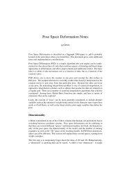
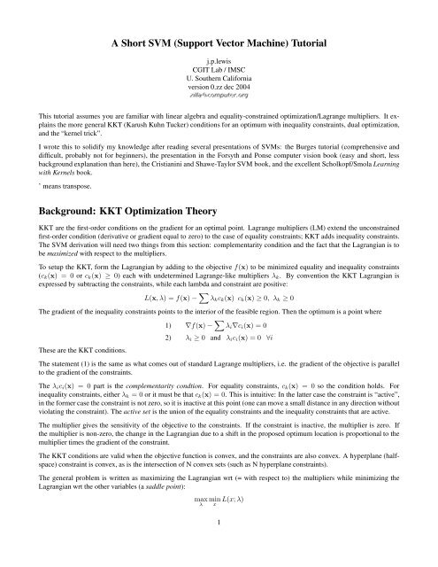
Figure 1: Maximum margin hyperplane
2

SVMs start from the goal of separating the data with a hyperplane, and extend this to non-linear decision boundaries using
the kernel trick described below. The equation of a general hyperplane is w ′ x + b = 0 with x being the point (a vector), w
the weights (also a vector). The hyperplane should separate the data, so that w ′ x k + b > 0 for all the x k of one class, and
w ′ x j + b < 0 for all the x j of the other class. If the data are in fact separable in this way, there is probably more than one way
to do it.
Among the possible hyperplanes, SVMs select the one where the distance of the hyperplane from the closest data points (the
“margin”) is as large as possible (Fig. 1). This sounds reasonable, and the resulting line in the 2D case is similar to the line I
would probably pick to separate the classes. The Scholkopf/Smola book describes an intuitive justification for this criterion:
suppose the training data are good, in the sense that every possible test vector is within some radius r of a training vector.
Then, if the chosen hyperplane is at least r from any training vector it will correctly separate all the test data. By making the
hyperplane as far as possible from any data, r is allowed to be correspondingly large. The desired hyperplane (that maximizes
the margin) is also the bisector of the line between the closest points on the convex hulls of the two data sets.
Now, find this hyperplane. By labeling the training points by y k ∈ −1, 1, with 1 being a positive example, −1 a negative
training example,
y k (w ′ x k + b) ≥ 0 for all points
Both w, b can be scaled without changing the hyperplane. To remove this freedom, scale w, b so that
y k (w ′ x k + b) ≥ 1 ∀k
Next we want an expression for the distance between the hyperplane and the closest points; w, b will be chosen to maximize
this expression. Imagine additional “supporting hyperplanes” (the dashed lines in Fig. 1) parallel to the separating hyperplane
and passing through the closest points (the support points). These are y j (w ′ x j + b) = 1, y k (w ′ x k + b) = 1 for some points
j, k (there may be more than one such point on each side).
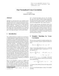
Figure 2: a - b = 2m
The distance between the separating hyperplane and the nearest points (the margin) is half of the distance between these support
hyperplanes, which is the same as the difference between the distances to the origin of the closest point on each of the support
hyperplanes (Fig. 2).
The distance of the closest point on a hyperplane to the origin can be found by minimizing x ′ x subject to x being on the
hyperplane,
minx ′ x + λ(w ′ x + b − 1)
x
d
= 0 = 2x + λw = 0
dx
→ x = − λ 2 w
3

now substitute x into w ′ x + b − 1 = 0 − λ 2 w′ w + b = 1
substitute this λ back into x
similarly working out for w ′ x + b = −1 gives
2(b − 1)
→ λ =
w ′ w
x = 1 − b
w ′ w w
x ′ x =
(1 − b)2
(w ′ w) 2 w′ w =
(1 − b)2
w ′ w
‖x‖ = √ x ′ x = √ 1 − b
w′ w = 1 − b
‖w‖
‖x‖ = −1 − b
‖w‖
Lastly, subtract these two distances, which gives the summed distance from the separating hyperplane to the nearest points:
2
‖w‖ .
To maximize this distance, we need to minimize w ... subject to all the constraints y k (w ′ x k + b) ≥ 1. Following the standard
KKT setup, use positive multipliers and subtract the constraints.
Taking the derivative w.r.t w gives
min
w,b L = 1 2 w′ w − ∑ λ k (y k (w ′ x k + b) − 1)
w − ∑ λ k y k x k = 0
or w = ∑ λ k y k x k . The sum for w above needs only be evaluated over the points where the LM is positive, i.e. the few
“support points” that are the minimum distance away from the hyperplane.
Taking the derivative w.r.t b gives
∑
λk y k = 0
This does not yet give b. By the KKT complementarity condition, either the lagrange multiplier is zero (the constraint is
inactive), or the L.M. is positive and the constraint is zero (active). b can be obtained by finding one of the active constraints
y k (w ′ x k + b) ≥ 1 where the λ k is non zero and solving w ′ x k + b − 1 = 0 for b. With w, b known the separating hyperplane
is defined.
Soft Margin classifier
In a real problem it is unlikely that a line will exactly separate the data, and even if a curved decision boundary is possible (as
it will be after adding the nonlinear data mapping in the next section), exactly separating the data is probably not desirable: if
the data has noise and outliers, a smooth decision boundary that ignores a few data points is better than one that loops around
the outliers.
This issue is handled in different ways by different flavors of SVMs. In the simplest() approach, instead of requiring
introduce “slack variables” s k ≥ 0 and allow
y k (w ′ x + b) ≥ 1
y k (w ′ x + b) ≥ 1 − s k
This allows the a point to be a small distance s k on the wrong side of the hyperplane without violating the stated constraint.
Then to avoid the trivial solution whereby huge slacks allow any line to “separate” the data, add another term to the Lagrangian
that penalizes large slacks,
min
w,b L = 1 2 w′ w − ∑ λ k (y k (w ′ x k + b) + s k − 1) + α ∑ s k
4

Reducing α allows more of the data to lie on the wrong side of the hyperplane and be treated as outliers, which gives a smoother
decision boundary.
Kernel trick
With w, b obtained the problem is solved for the simple linear case in which the data are separated by a hyperplane. The “kernel
trick” allows SVMs to form nonlinear boundaries. There are several parts to the kernel trick.
1. The algorithm has to be expressed using only the inner products of data items. For a hyperplane test w ′ x this can be done
by recognizing that w itself is always some linear combination of the data x k (“representer theorem”), w = ∑ λ k x k , so
w ′ x = ∑ λ k x k x.
2. The original data are passed through a nonlinear map to form new data with additional dimensions, e.g. by adding the
pairwise product of some of the original data dimensions to each data vector.
3. Instead of doing the inner product on these new, larger vectors, think of storing the inner product of two elements x ′ j x k
in a table k(x j ,x k ) = x ′ j x k, so now the inner product of these large vectors is just a table lookup. But instead of doing
this, just “invent” a function K(x j ,x k ) that could represent dot product of the data after doing some nonlinear map on
them. This function is the kernel.
These steps will now be described.
Kernel trick part 1: dual problem. First, the optimization problem is converted to the “dual form” in which w is eliminated
and the Lagrangian is a function of only λ k . To do this substitute the expression for w back into the Lagrangian,
L = 1 2 w′ w − ∑ λ k (y k (w ′ x k + b) − 1)
w = ∑ λ k y k x k
L = 1 2 (∑ λ k y k x k ) ′ ( ∑ λ l y l x l ) − ∑ λ m (y m (( ∑ λ n y n x ′ n) ′ x m + b) − 1)
= 1 2
∑∑
λk λ l y k y l x ′ kx l − ∑∑ λ m λ n y m y n x ′ mx n − ∑ λ m y m b + ∑ λ m
the term ∑ λ m y m b = b ∑ λ m y m is zero
because dL
db gave ∑ λ m y m = 0 above.
so the resulting dual Lagrangian is L D = ∑ λ m − 1 2
∑ ∑
λk λ l y k y l x ′ k x l
subject to λ k > 0
∑
and λk y k = 0
To solve the problem the dual L D should be maximized wrt λ k as described earlier.
The dual form sometimes simplifies the optimization, as it does in this problem - the constraints for this version are simpler
than the original constraints. One thing to notice is that this result depends on the 1/2 added for convenience in the original Lagrangian.
Without this, the big double sum terms would cancel out entirely! For SVMs the major point of the dual formulation,
however, is that the data (see L D ) appear in the form of their dot product x ′ k x l. This will be used in part 3 below.
Kernel trick part 2: nonlinear map. In the second part of the kernel trick, the data are passed through a nonlinear mapping.
For example in the two-dimensional case suppose that data of one class is near the origin, surrounded on all sides by data of the
second class. A ring of some radius will separate the data, but it cannot be separated by a line (hyperplane).
The x, y data can be mapped to three dimensions u, v, w:
u ← x
v ← y
w ← x 2 + y 2
5

The new “invented” dimension w (squared distance from origin) allows the data to now be linearly separated by a u − v plane
situated along the w axis. The problem is solved by running the same hyperplane-finding algorithm on the new data points
(u, v, w) k rather than on the original two dimensional (x, y) k data. This example is misleading in that SVMs do not require
finding new dimensions that are just right for separating the data. Rather, a whole set of new dimensions is added and the
hyperplane uses any dimensions that are useful.
Kernel trick part 3: the “kernel” summarizes the inner product. The third part of the “kernel trick” is to make use of
the fact that only the dot product of the data vectors are used. The dot product of the nonlinearly feature-enhanced data
from step two can be expensive, especially in the case where the original data have many dimensions (e.g. image data) – the
nonlinearly mapped data will have even more dimensions. One could think of precomputing and storing the dot products in a
table K(x j ,x k ) = x ′ j x k, or of finding a function K(x j ,x k ) that reproduces or approximates the dot product.
The kernel trick goes in the opposite direction: it just picks a suitable function K(x j ,x k ) that corresponds to the dot product
of some nonlinear mapping of the data. The commonly chosen kernels are
(x ′ j,x k ) d , d = 2 or 3
exp(−‖x j − x k ‖) 2 /σ
tanh(x ′ j x k + c)
Each of these can be thought of as expressing the result of adding a number of new nonlinear dimensions to the data and then
returning the inner product of two such extended data vectors.
A SVM is the maximum margin linear classifier (as described above) operating on the nonlinearly extended data. The particular
nonlinear “feature” dimensions added to the data are not critical as long as there is a rich set of them. The linear classifier will
figure out which ones are useful for separating the data. The particular kernel is to be chosen by trial and error on the test set,
but on at least some benchmarks these kernels are nearly equivalent in performance, suggesting the choice of kernel is not too
important.
6