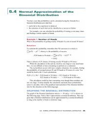
Pg 465

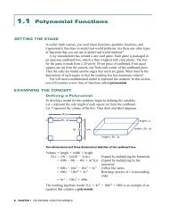
6.4 Finding Optimal Values for
Composite Function Models
SETTING THE STAGE
You have used calculus to solve many real-world problems involving
polynomial, rational, and now composite functions. In these problems, you are
often asked to minimize distance, time, or cost. For example,
George wants to run a power line to a new cottage being built on an island
that is 400 m from the shore of a lake. The main power line ends 3 km away
from the point on the shore that is closest to the island. The cost of laying the
power line under water is twice the cost of laying the power line on land.
How should George place the line to minimize the overall cost
In this section, you will revisit the techniques you learned for solving
optimization problems in Chapters 4 and 5. You will apply these techniques to
composite function models.
EXAMINING THE CONCEPT
Solving Optimization Problems Involving
the Chain Rule
Before solving the power line problem, consider some simpler examples.
Recall the strategy for solving optimization problems in section 4.5
on page 305.
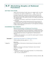
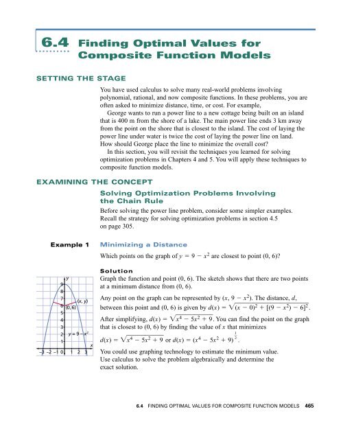
Example 1
9
8
7
6
5
4
3
2
1
–3 –2 –1 0
y
(x, y)
(0, 6)
y = 9 – x 2
1 2 3
x
Minimizing a Distance
Which points on the graph of y 9 x 2 are closest to point (0, 6)
Solution
Graph the function and point (0, 6). The sketch shows that there are two points
at a minimum distance from (0, 6).
Any point on the graph can be represented by (x, 9 x 2 ). The distance, d,
between this point and (0, 6) is given by d(x) (x ) 09 2 [( ) x 2 6]
2 .
After simplifying, d(x) x x 4 5. 2 9 You can find the point on the graph
that is closest to (0, 6) by finding the value of x that minimizes
d(x) xx 4 5
2 9
or d(x) (x 4 5x 2 9) .
You could use graphing technology to estimate the minimum value.
Use calculus to solve the problem algebraically and determine the
exact solution.
1
2
6.4 FINDING OPTIMAL VALUES FOR COMPOSITE FUNCTION MODELS 465

d′(x) d
d
x
(x 4 5x 2
9) 2
d(x 4 5x 2 2
9)
d(x 4 5x 2 9)
1
1
d
• d
(x
x
4 5x 2 9)
Apply the chain rule.
1 2 (x4 5x 2 9)
d
• d
(x
x
4 5x 2 9)
• (4x 3 10x) Factor the numerator.
2x(2x 2 5)
1
2(x 4 5x 2 9)
2
x(2x 2 5)
Simplify.
x x 4 5
2 9
The derivative is a rational expression. To find the critical numbers, determine
where d′(x) 0 or d′(x) does not exist. The only case in which d′(x) cannot
exist is when the denominator, x x 4 5, 2 9 is equal to 0. However, this case
cannot occur, as is shown below.
x 4 5x 2 9 x 2 5 2 2 1 1
Complete the square.
4
For all x ∈ R,x 2 5 2 2 ≥ 0.
∴ x2 5 2 2 1 1
> 0
4
1
2(x 4 5x 2 9)
1
2
1
2
∴ x x 4 5 2 9 > 0.
Thus, d′(x) is defined for all values of x ∈ R. Also, d′(x) 0 when the
numerator, x(2x 2 5), equals 0; that is, when x 0 or x ±
5 2 .
Solving x 0 and 2x 2 5 0 produces the critical numbers. Therefore, the
critical numbers are x
5 2 , x 0, and x 5 2 . Apply the first derivative
test to find the critical numbers that represent a local minimum.
Intervals
x < –
5 2 –
5 2 < x < 0 0 < x < 5 2 x >
5 2
x – – + +
(2x 2 – 5) + – – +
xx 4 – 5 2 + 9 + + + +
d′(x) (– )(+
( +
)
)
= – (– )(
( +
–)
)
= + (+ )(
(+ –)
)
= – (+ )(
+)
( = +
+ )
→
d (x) decreasing increasing decreasing increasing
→
minimum at x = –
5 2 maximum at x = 0 minimum at x = 5 2
→
→
466 CHAPTER 6 RATES OF CHANGE IN COMPOSITE FUNCTION MODELS

The first derivative test verifies that a local minimum occurs when x
5 2 or
x
5 2 . These values correspond to the minimum distance. Substitute them
into the original function y 9 x 2 to get the minimum distance, which is the
corresponding value of the function.
y 9
5 2 2 and y 9 5 2 2
9 5 2
9 5 2
1 3 13
2
2
The two points closest to (0, 6) on the graph of y 9 x 2 are 5 2 , 1 2
and 5 2 , 1 3
2 .
Note that in this case, the calculator cannot be used to determine an exact
solution, but can be used to check the reasonableness of the solution by
evaluating
5 2 and comparing with the graphs above.
3
Example 2
Deciding When Two Moving Objects Are Closest
to Each Other
A north–south highway intersects an east–west highway at point P. A vehicle
crosses P at 1:00 p.m., travelling east at a constant speed of 60 km/h. At the
same instant, another vehicle is 5 km north of P, travelling south at 80 km/h.
Find the time when the two vehicles are closest to each other and the distance
between them at that time.
80t
5 – 80t
North
5 km north of P
P
Q
d
60t
R
East
Solution
Draw a diagram. Let the x- and y-axes be the highways, and let P be at the
origin. The slower vehicle is travelling away from P, while the faster
vehicle is travelling toward P.
Let t be the number of hours after 1:00 P.M.
At time t, the slower vehicle is 60t kilometres east of P, and the faster
vehicle is (5 80t) kilometres north of P.
The quantity to be minimized is the distance between the two vehicles, d.
From the diagram and using the Pythagorean theorem,
d 2 (5 80t) 2 (60t) 2
d 2 25 800t 10 000t 2
d 25 00t – 810 t 000
2
∴ d(t) (25 800t 10 000t 2 )
You can estimate the solution graphically, as shown. The minimum
distance, approximately 3 km, occurs at t 0.04.
1
2
6.4 FINDING OPTIMAL VALUES FOR COMPOSITE FUNCTION MODELS 467

Use calculus to calculate the exact solution algebraically. Applying the chain
rule and the power rule,
d′(t)
1 2 (25 800t 10 000t2 )
d
• d
(25 800t 10 000t
t
2 )
d
• d
(25 800t 10 000t
t
2 )
1 2 (25 800t 10 000t2 ) • (800 20 000t)
d(25 800t 10 000t 2 )
2
d(25 800t 10 000t 2 )
800 20 000t
1
2(25 800t 10 000t 2 )
2
400 10 000t
25 00t 810 t 000
2
Critical numbers occur when d′(t) 0 or is undefined. Note that the
denominator equals (100t
4) 2 9, which is always greater than 0;
therefore, the derivative is always defined. So, d′(t) 0 when the numerator
equals 0.
∴ 0 400 10 000t
t 0.04
1
Use the first derivative test to verify that t 0.04 represents a local minimum.
The first derivative test confirms that a local minimum occurs when t 0.04.
In this case, the calculator gives the exact solution.
The distance between the vehicles is minimized at this time. The value t 0.04
means 0.04 h, or 0.04 60 2.4 min, or 2 min 24 sec.
Evaluate d when t 0.04 to determine the minimum distance.
d(0.04) 25 00(0.0 84) 0 10.04) 000(
2
3
The two vehicles are closest to each other when they are 3 km apart at exactly
1:02:24 P.M.
1
2
1
2
Intervals
0 ≤ t < 0.04 t > 0.04
–400 + 10 000t – +
25 00t – 810 + 0t 00 2 +
(–)
d′(t) (
= – ( + )
= +
+ )
( + )
d(t) decreasing increasing
→
minimum at x = 0.04
→
468 CHAPTER 6 RATES OF CHANGE IN COMPOSITE FUNCTION MODELS

Example 3
Minimizing the Cost of an Electrical Power Line
Recall the problem in Setting the Stage.
George wants to run a power line to a new cottage being built on an island
that is 400 m from the shore of a lake. The main power line ends 3 km away
from the point on the shore that is closest to the island. The cost of laying the
power line under water is twice the cost of laying the power line on land. How
should George place the line to minimize the overall cost
Solution
Sketch a diagram of the situation. The cable will run along the shore, enter the
water at some point, and continue straight to the island.
400 m
3000 m
end of existing
power line
x
L1
L 2
1 2
Let x represent the distance between the point on the shore closest to the island
and the point where the cable enters the water. Let L 1
represent the length of
cable underwater and L 2
the length of cable on land. Therefore, the total cost to
lay the cable is C 2L 1
L 2.
Minimize this quantity, C.
From the diagram, L 2
3000 x and (L 1
) 2 x 2 400 2 , so
L 1
x 60 2 1. 000 Substituting in the expression for C gives
C(x) 2(x 60 2 1) 000 (3000 x)
∴ C(x) 2(x 2 160 000) (3000 x) 0 ≤ x ≤ 3000
You can estimate the minimum value using graphing technology.
Now use calculus to calculate the exact solution algebraically.
Using the difference and chain rules,
C′(x) d
d
x
2(x 2 160 000) d
d[2(x 2 160 000) ]
d(x 2 160 000)
d
x
d
(3000) d
(x)
C′(x) • 0 1
2 1 2 (x2 160 000)
(x 2 160 000) • 2x 1
2x
1
2
1
2
d(x 2 160 000)
dx
d
• d
(x
x
2 160 000) 1
1
x 60 2 1000
Critical numbers occur when C′(x) equals 0 or is undefined. In this case, the
denominator is always greater than 0, so C′(x) is defined for all x where
0 < x < 3000. Solve for x to determine where C′(x) 0.
1 2
1 2
x
6.4 FINDING OPTIMAL VALUES FOR COMPOSITE FUNCTION MODELS 469

2x
x 60 2 1000
2x
x 60 2 1 000
1 0
1
2x x 60 2 1000
4x 2 x 2 160 000
3x 2 160 000
00
0
x ±
160 3
x 230.94
Add 1 to each side.
Multiply each side by x 60 2 1.
000
Square both sides.
Isolate x 2 .
Solve for x.
Since x ≥ 0, the negative solution is
inadmissible.
Intervals
0 ≤ x < 230.94 230.94 < x ≤ 3000
C ′(x) – +
C(x) decreasing increasing
The first derivative test confirms that a global minimum occurs at x 230.94.
This value is the distance from the point on the shore closest to the island to the
point where the cable enters the water. This distance will minimize the cost of
installing the cable. Using this value, calculate L 1
and L 2
.
L 1
(230.9 4) 160 2 0 00 L 2
3000 230.94
461.88 2769.06
The total cost of laying the cable is minimized if about 2769.06 m are placed
along the shore and 461.88 m are placed underwater.
→
minimum at x = 230.94
→
CHECK, CONSOLIDATE, COMMUNICATE
1. Why do optimization problems involving distance often result in using
the chain rule
2. Suppose you have found the model for a problem. Is determining the
optimal values of a composite function different from determining the
optimal values for polynomial and rational functions Explain your
answer in terms of techniques.
KEY IDEAS
• The properties of the derivative that you use to solve optimization
problems involving composite functions are the same as those you apply
to polynomial and rational functions.
• Use the strategy for solving optimization problems, outlined in Chapters 4
and 5 on pages 305 and 397, to also solve problems involving composite
function models.
470 CHAPTER 6 RATES OF CHANGE IN COMPOSITE FUNCTION MODELS

6.4 Exercises
A
1. Find the point on the line y 6x 8 that is closest to the origin, (0, 0).
2. What point on the graph of f (x) x 2 is closest to (2, 0.5)
3. Find the point on the curve 2y 2 4(x 1) that is closest to the origin.
4. Ship A, sailing due east at 8 km/h, sights ship B 5 km to the southeast when
ship B is sailing due north at 6 km/h. How close to each other will the two
ships be when they pass
5. Mike, who is standing on the deck of a yacht that is travelling due west at
6 km/h, sees a sailboat sailing southwest at 4 km/h, 3 km northwest of the
yacht. How close to each other do these boats get
6. Knowledge and Understanding: Determine the points on the curve
y x, 0≤ x ≤ 1, that are (a) closest to and (b) farthest from point (2, 0).
B
7. A passenger jet is travelling due north at 400 km/h, while a cargo plane,
2 km to the northwest, is travelling east at 300 km/h. The altitude of the
cargo plane is 1000 m lower than the altitude of the passenger jet. What will
be the minimum separation between the two aircraft
8. A truck travelling west at 100 km/h is 250 km due east of a sports car going
north at 120 km/h. When will the vehicles be closest to each other What is
the minimum distance between them
9. A boat leaves a dock at 2:00 P.M., heading west at 15 km/h. Another boat
heads south at 12 km/h and reaches the same dock at 3:00 P.M. When were
the boats closest to each other
West
R
North
100t
Q
10 km
d 10 – 100t
P
80t
10. Communication: Devise an optimization problem based on the diagram on
the left.
11. A woman lives on an island 2 km from the mainland. Her fitness club is
4 km along the shore from the point closest to the island. To get to the
fitness club, she paddles her kayak at 2 km/h. Once she reaches the shore,
she jogs at 4 km/h. Determine where she should land to reach her fitness
club in the shortest possible time.
12. A dune buggy is on a straight desert road, 40 km north of Dustin City. The
vehicle can travel at 45 km/h off the road and 75 km/h on the road. The
driver wants to get to Gulch City, 50 km east of Dustin by another straight
road, in the shortest possible time. Determine the route he should take.
13. Suppose you are swimming in a lake and find yourself 200 m from shore.
You would like to get back to the spot where you left your towel, which is
at least 200 m down the beach, as quickly as possible. You can walk along
the beach at 100 m/min, but you can swim at only 50 m/min. To what point
on the beach should you swim to minimize your total travelling time
6.4 FINDING OPTIMAL VALUES FOR COMPOSITE FUNCTION MODELS 471

Ancaster
4
rest
stop
C 8
Dundas
D
C
6
14. The owners of a small island want to bring in electricity from the mainland.
The island is 80 m from a straight shoreline at the closest point. The nearest
electrical connection is 200 m along the shore from that point. It costs twice
as much to install cable across water than across land. What is the least
expensive way to install the cable
15. Application: Bill owns an oil well located 400 m from a road. Bill wants
to connect the well to a storage tank 1200 m down the road from the well.
It costs $35/m to lay pipe along the road and $50/m to lay it elsewhere.
How should the pipeline be laid to minimize the total cost
16. Thinking, Inquiry, Problem Solving: Find the dimensions of the rectangle of
x
2 2
maximum area that can be inscribed in the ellipse 1
1.
y 6 9
17. Check Your Understanding: Is the strategy for solving optimization
problems different for rational and composite function models Explain.
18. An offshore oil well is in the ocean at a point 5 km from the closest point
on a straight shoreline. The oil must be pumped from the well to a storage
facility on shore. The storage facility is 15 km away from the point on shore
that is closest to the well. It costs $100 000/km to lay pipe underwater and
$75 000/km over land. How should the pipeline be situated on the shore to
minimize the cost
19. Prove that (1, 0) is the closest point on the circle x 2 y 2 1 to (2, 0).
20. Two towns, Ancaster and Dundas, are 4 km and 6 km, respectively, from
an old railroad line that has been made into a bike trail. Points C and D
on the trail are the closest points to the two towns, respectively. These
points are 8 km apart. Where should a rest stop be built to minimize the
length of new trail that must be built from both towns to the rest stop
ADDITIONAL ACHIEVEMENT CHART QUESTIONS
Knowledge and Understanding: A north–south highway intersects an east–west
highway at point P. A vehicle passes P at 3:00 P.M., travelling east at a constant
speed of 100 km/h. At the same instant, another vehicle passes 2 km north of P,
travelling south at 80 km/h. Find the time when the two vehicles are closest to
each other and when the distance between them is minimal.
10 km
Application: Millie is in a boat 2 km from a straight shoreline and wants to reach
a point on the shore 10 km north of her present position, as shown in the
diagram. She can row at 5 km/h and jog at 8 km/h. Calculate the position on the
shoreline to which she should row to reach the destination in the shortest time.
Thinking, Inquiry, Problem Solving: Find the area of the largest rectangle that
can be inscribed in a circle with radius r.
2 km
Communication: To solve an optimization problem, you set the derivative of the
function that models the problem to 0 and solve the resulting equation. Why
472 CHAPTER 6 RATES OF CHANGE IN COMPOSITE FUNCTION MODELS