PHY–396 K. Solutions for problem set #6. Problem 1(a): The theory ...

PHY–396 K. Solutions for problem set #6.
Problem 1(a):
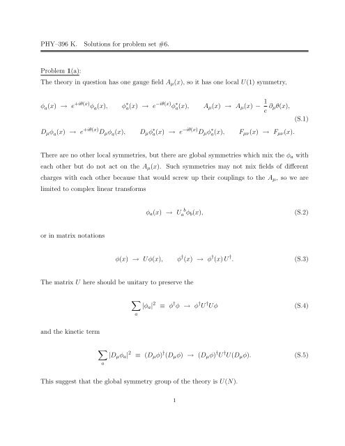
The theory in question has one gauge field A µ (x), so it has one local U(1) symmetry,
φ a (x) → e +iθ(x) φ a (x), φ ∗ a(x) → e −iθ(x) φ ∗ a(x), A µ (x) → A µ (x) − 1 e ∂ µθ(x),
D µ φ a (x) → e +iθ(x) D µ φ a (x), D µ φ ∗ a(x) → e −iθ(x) D µ φ ∗ a(x), F µν (x) → F µν (x).
(S.1)
There are no other local symmetries, but there are global symmetries which mix the φ a with
each other but do not act on the A µ (x). Such symmetries may not mix fields of different
charges with each other because that would screw up their couplings to the A µ , so we are
limited to complex linear transforms
φ a (x) → U b
a φ b (x),
(S.2)
or in matrix notations
φ(x) → Uφ(x), φ † (x) → φ † (x) U † . (S.3)
The matrix U here should be unitary to preserve the
∑
|φ a | 2 ≡ φ † φ → φ † U † Uφ (S.4)
a
and the kinetic term
∑
|D µ φ a | 2 ≡ (D µ φ) † (D µ φ) → (D µ φ) † U † U(D µ φ). (S.5)
a
This suggest that the global symmetry group of the theory is U(N).
1

Mathematically, the U(N) group is a direct product SU(N) × U(1) where the SU(N)
factor comprises matrices with unit determinant while the U(1) factor corresponds to
φ a (x) → e +iθ φ a (x), φ ∗ a(x) → e −iθ φ ∗ a(x), sameθ ∀a. (S.6)
Clearly, such global U(1) transforms are simply special cases of the local U(1) symmetry (S.1)
for θ(x) = const, so they do not make a separate global symmetry. Therefore, the global
symmetry group of the theory is SU(N) rather than U(N).
Problem 1(b):
According to part (a), symmetries act on scalar fields as
φ a (x) → e iθ(x) U b
a φ b (x), U = const, U † U = 1. (S.7)
To preserve the vacuum expectation values 〈φ a 〉 = vδ a,N such a transform must have
(α)
(β)
U N
i = 0 for i = 1, . . . , (N − 1),
U N
N
× eiθ(x) ≡ 1 ∀x.
Condition (β) implies θ = const, so all symmetries preserving the VEVs are global rather
than local.
For a unitary matrix U, condition (α) requires U to be block-diagonal,
U =
⎛
⎜
⎝
⎞
0
Ũ .
⎟
0 ⎠
0 · · · 0 e −iξ
(S.8)
where Ũ is a unitary (N − 1) × (N − 1) matrix and ξ is some real phase. To satisfy (β) we
need ξ = θ, and we also need det(U) = det(Ũ) × e−iξ = 1. Consequently, Ũ = eiξ/(N−1) × W
where det W = 1.
2

Altogether, we have unbroken symmetries acting on the fields as
φ N (x) → φ N (x),
N−1
∑
φ i (x) → e iNξ/(N−1)
j=1
W j
i
φ j (x),
W ∈ SU(N − 1), e iξ ∈ U(1), same W and e iξ ∀x. (S.9)
These are global symmetries, and the group is SU(N − 1) × U(1).
Problem 1(c): The symmetry group of the theory G = SU(N) × U(1) ∼ = U(N) has N 2
generators. The group of unbroken symmetries H = SU(N −1)×U(1) ∼ = U(N −1) has (N −1) 2
generators. Consequently, the spontaneously broken symmetries comprise U(N)/U(N − 1),
and the number of broken generators is N 2 − (N − 1) 2 = 2N − 1. Had all the symmetries
were global, this would require 2N − 1 massless Goldstone scalars.
However, one of the broken symmetries is local rather than global, and the corresponding
Goldstone scalar is eaten up by the Higgs mechanism which makes the vector field A µ massive.
This leaves us with only 2N − 2 massless Goldstone scalars.
To determine their U(N − 1) quantum numbers we need a little group theory. A nonabelian
symmetry group acts non-trivially on its own generators, T α → UT α U −1 ≠ T α .
However, the generators transform linearly into each other; together, they form an adjoint
multiplet where
T α → UT α U −1 = ∑ β
Adj(U) α,β × T β .
(S.10)
For the U(N) group, the adjoint multiplet is equivalent to N × N where N is the fundamental
multiplet of the group (N complex members) and N is its complex conjugate. In other words,
we may label the N 2 generators of the U(N) as T b
a , and they transform into each other exactly
as the field products φ a × φ ∗b . The unbroken U(N − 1) symmetry is generated by the T j
i
with i, j < N; naturally, these generators form the adjoint multiplet of the U(N − 1). The
remaining, broken generators are as follows:
• The T N
i with i < N, which comprise the fundamental N − 1 multiplet of the U(N − 1).
3

• The T j
N
U(N − 1).
with j < N, which comprise the anti-fundamental N − 1 multiplet of the
• The TN N , which is a singlet of the U(N − 1).
Thus, we expect N − 1 charged Goldstone scalars in a fundamental N − 1 multiplet of
the U(N − 1). Their antiparticles make an anti-fundamental N − 1 multiplet. For a global
U(N) symmetry there would also be a neutral Goldstone boson in a singlet multiplet of the
U(N − 1), but because the U(1) symmetry is global, this singlet is eaten up by the Higgs
mechanism: It becomes the longitudinal polarization of the massive vector instead of a scalar
particle of its own right.
PS: The above counting of broken generators and Goldstone bosons is correct, but the full
story of the singlet is a bit more complicated. Because the U(N) group is not simple but a
product SU(N) × U(1), the adjoint multiplet of the U(N) is reducible. The U(1) generator
∑a T a
a
is a singlet, while the remaining N 2 − 1 combinations of the T b
a
multiplet of the SU(N).
form the adjoint
From the unbroken U(N − 1) = SU(N − 1) × U(1) point of view, the adjoint of the
U(N) contains two singlets, the ∑ a T a
a
∈ Adj[U(1) local ] and the ∑ i T i
i
− (N − 1)T N
N
Adj[SU(N) global ]. One linear combination of these two singlets — namely the TN
N — is
broken by the VEV 〈φ N 〉 ̸= 0, while the other combination ∑ i T i
i remains unbroken, but
only as a global symmetry. But despite this mixing of the two singlets, the overall symmetry
breaking pattern
∈
U(N − 1) singlets : 1 local + 1 global → 1 broken + 1 global (S.11)
has the same effect as if there was only one singlet, which used to generate a local symmetry
but became spontaneously broken. Consequently, there are no SU(N − 1)–singlet Goldstone
particles; instead, one real scalar field becomes eaten by the Higgs mechanism when the A µ
field becomes massive.
4

Problem 1(d):
For m 2 < 0, the scalar potential
V = λ 4 (φ† φ) 2 + m 2 φ † φ (S.12)
is minimized for
φ † φ = v2
2 = −2m2
λ
> 0. (S.13)
These minima for a sphere in the field space, and without loss of generality, we work with the
vacuum states where fields’ expectation values lie at the “North pole” of this sphere,
〈φ N 〉 = v × δ a,n . (S.14)
The excited states near this vacuum have φ N (x) ≠ 0 (expect along some singular lines, which
should be few and far between), so we may impose a unitary gauge for the vector fields by
requiring
phase (φ N (x)) ≡ 0 ∀x. (S.15)
Note that the phases of the remaining φ i (x) fields remain unconstrained.
Now let’s shift the φ N field by its VEV,
φ N (x) = v + σ(x) √
2
,
while the remaining φ i (x) scalars stay as they are. In terms of the real σ(x) field and the
complex φ i (x) fields, the scalar potential becomes
V = const + λ 4
( ∑
i
|φ i | 2 +
(v + σ)2
2
) 2
− v2
2
= const + λv2
4 × σ2 + cubic + quartic.
(S.16)
The kinetic terms |D µ φ i | 2 of the un-shifted φ i fields remain as they are, but the kinetic term
5

for the φ N becomes
|D µ Φ N | 2 = 1 2 |∂ µσ + eA µ (v + σ)| 2 =
2 1(∂ µσ) 2 + e2 (v + σ) 2
A µ A µ .
2
(S.17)
Altogether, we have
L = − 1 4 F µνF µν + e2 (v + σ) 2
A µ A µ
2
+ ∑ i
|∂ µ φ i + ieA µ φ i | 2 + 1 2 (∂ µσ) 2 − V (σ, |φ i |)
= const + L 2 + L 3+4
(S.18)
where the quadratic terms in
L 2 = − 1 4 F µνF µν + e2 v 2
2 A µA µ + ∑ i
|∂ µ φ i | 2 + 1 2 (∂ µσ) 2 − λv2
4 σ2 (S.19)
determines the particles of the theory, while the cubic and quartic terms in the L 3+4 govern
their interactions. Specifically, the quadratic Lagrangian (S.19) describes:
• One massive vector field A µ of mass = ev.
• One massive neutral scalar field σ of mass 2 = 1 2 λv2 = −2m 2 > 0.
• N − 1 charged massless scalar fields φ i . These are the Goldstone bosons of the broken
global symmetries.
Problem 2(e):
A charged quantum field such as ˆφ i (x) together with its hermitian conjugate ˆφ † i
(x) describe
a particle and a distinct antiparticle. The ˆφ i (x) comprises operators which create particles
or annihilate antiparticles, while the ˆφ † i
(x) comprises operators which create antiparticles or
annihilate particles.
For the problem at hand, the N − 1 charged scalar fields ˆφ i create and annihilate 2 ×
(N − 1) massless particles species, the N − 1 multiplet of particles, and the N − 1 multiplet
of antiparticles. Clearly, these are precisely the Goldstone particles we expect from part (c).
Q.E.D.
6

Problem 2(a):
given Φ → e +iθ U L ΦU † R , (4)
we have Φ † → e −iθ U R Φ † U † L , (S.20)
hence Φ † Φ → U R (Φ † Φ)U † R , (S.21)
(
Φ † Φ ) 2 → UR Φ † ΦU † R U RΦ † ΦU † R = U R(
Φ † Φ ) 2 U
†
R , (S.22)
(
likewise Φ † Φ ) n (
→ UR Φ † Φ ) n U
†
R
∀n = 1, 2, 3, . . . , (S.23)
and therefore
all traces tr
( (Φ † Φ ) n ) are invariant under (4), (S.24)
thanks to the cyclic invariance rule for traces. ⋆
invariant under symmetries (4).
Consequently, the scalar potential (3) is
For the global symmetries where e iθ , U L , and U R do not depend on x, the kinetic term
in (2) is also invariant. Indeed,
for constant e iθ , U L , U R ,
∂ µ Φ → e +iθ U L (∂ µ Φ)U † R ,
∂ µ Φ † → e −iθ U R (∂ µ Φ † )U † L ,
(S.27)
∂ µ Φ † ∂ µ Φ → U R (∂ µ Φ † ∂ µ Φ)U † R ,
and tr ( ∂ µ Φ † ∂ µ Φ ) is invariant.
Q.E.D.
⋆ Trace of a product of two matrices does not depend on the order of multiplication, tr(AB) = tr(BA).
Consequently, trace of a product of several matrices is not affected by cyclic permutations of the factors,
tr(ABC · · · XY Z) = tr(BC · · · XY ZA) = tr(C · · · XY ZAB) = · · · = tr(ZABC · · · XY ).
(S.25)
In particular, for any unitary matrix U and any matrix A,
tr(UAU † ) = tr(AU † U) = tr(A).
(S.26)
The invariance (S.24) follows from eq. (S.23) by this rule.
7

Problem 2(⋆):
The kinetic term in (2) and the last two terms in the potential (3) have a much bigger
symmetry than G, namely SO(2N 2 ), which does not care for the matrix structure of the Φ(x)
and treats it as 2N 2 real component fields. Indeed,
(
tr Φ † Φ) = ∑ i,j
∣
∣Φ j
i
∣
∣ 2
= ∑ i,j
( ( ) 2 ( ) ) 2
Re Φ j
i + Im Φ j
i
(S.28)
is invariant under all SO(2N 2 ) “rotations” of the components, and so is the kinetic term.
On the other hand, the tr ( Φ † Φ Φ † Φ ) in the potential does depend on the packing of 2N 2
real components into a complex N × N matrix, and it is this term which reduces the internal
symmetry group of the theory to G = SU(N) × SU(N) × U(1).
Proving that all the SO(2N 2 )/G symmetries are broken by the quartic trace term is a
non-trivial exercise in group theory rather than field theory. You do not have to do it as part
of this homework set, and I am not writing down the proof here.
Problem 2(b):
Given the eigenvalues (κ 1 , . . . , κ N ) of the Φ † Φ matrix, the invariant traces (S.24) obtain as
tr
( (Φ † Φ ) n ) =
N∑
κ n i .
i=1
(S.29)
Consequently, the scalar potential is
( ∑
i
V = α 2
∑
κ 2 i + β 2
i
κ i
) 2
+ m 2 ∑ i
κ i .
(S.30)
Now let’s minimize this potential. Since the matrix Φ † Φ cannot have any negative eigenvalues,
we are looking for a minimum of V (κ 1 , . . . , κ N ) under constraints κ i ≥ 0. This requires
∀i = 1, . . . , N,
either κ i ≥ 0 and ∂V
∂κ i
= 0, or else κ i = 0 and ∂V
∂κ i
> 0, (S.31)
8

where
∂V
∂κ i
= ακ i + m 2 + β ∑ j
κ j .
(S.32)
The solutions of these equations are as follows:
• For α > 0, β > 0, and m 2 > 0, the only solution is κ 1 = · · · κ N = 0 and hence 〈Φ〉 = 0.
• For α > 0, β > 0, and m 2 < 0, the only solutions is (5) and hence 〈Φ〉 = C × a unitary
matrix. We shall focus on this regime in parts (c–e) of this problem and in problem 3.
• For α < 0 or β < 0, the situation is more complicated:
— When α + β < 0 or α + Nβ < 0, the scalar potential (3) is unbounded from below
and the theory is sick.
— When α > 0 and β < 0 but α + Nβ > 0, the solutions are similar to the β > 0 case:
For m 2 > 0 all κ i = 0, while for m 2 < 0 the κ i are as in eq. (5).
— When β > 0 and α < 0 but α+β > 0, there is only one 〈φ〉 = 0 solution for m 2 > 0,
but there are N distinct solutions for m 2 < 0, namely for k = 1, 2, . . . , N,
κ 1 = · · · = κ k = −m2
α + kβ > 0, κ k+1 = · · · = κ N = 0 (S.33)
(modulo permutations of the eigenvalues). The deepest minimum of V corresponds
to the k = 1 solution.
Problem 2(c):
Let’s act with some SU(N) L × SU(N) R × U(1) symmetry (4) on the vacuum expectation
values (6):
〈Φ〉 = C × 1 N×N → e iθ U L 〈Φ〉 U † R = C × eiθ U L U † R . (S.34)
Clearly, to keep the VEVs 〈Φ〉 invariant, we need
e iθ U L U † R = 1 N×N (S.35)
9

and hence
U R = e iθ × U L . (S.36)
Moreover, since the U L and U R matrices have unit determinants, this means
e iθ = 1 and U L = U R ∈ SU(N). (S.37)
In other words, the unbroken symmetry group is SU(N) which acts on the scalar fields as
Φ(x) → UΦ(x) U † , U ∈ SU(N). (S.38)
Problem 2(d):
In terms of the shifted fields (7),
∂ µ Φ = 1 √
2
(∂ µ ϕ 1 + i∂ µ ϕ 2 ) , ∂ µ Φ † = 1 √
2
(∂ µ ϕ 1 − i∂ µ ϕ 2 ) ,
(S.39)
hence the kinetic term in the Lagrangian becomes
tr ( ∂ µ Φ † ∂ µ Φ ) = 1 2 tr(∂ µϕ 1 ∂ µ ϕ 1 ) + 1 2 tr(∂ µϕ 2 ∂ µ ϕ 2 ).
(S.40)
As to the potential terms,
tr ( Φ † Φ ) = NC 2 + √ 2C tr(ϕ 1 ) + 1 2 tr(ϕ2 1) + 1 2 tr(ϕ2 2),
tr 2( Φ † Φ ) = N 2 C 4 + 2 √ 2NC 3 tr(ϕ 1 ) + 2C 2 tr 2 (ϕ 1 ) + NC 2 ( tr(ϕ 2 1) + tr(ϕ 2 2) )
+ √ 2C tr(ϕ 1 ) × ( tr(ϕ 2 1) + tr(ϕ 2 2) ) + 1 4
tr
( (Φ † Φ ) 2 ) = NC 4 + 2 √ 2C 3 tr(ϕ 1 ) + 3C 2 tr(ϕ 2 1) + C 2 tr(ϕ 2 2)
+ √ 2C tr(ϕ 3 1) + √ 2C tr(ϕ 1 ϕ 2 2)
(
tr(ϕ
2
1 ) + tr(ϕ 2 2) ) 2
and therefore
+ 1 4 tr(ϕ4 1) + 1 4 tr(ϕ4 2) + 3 2 tr(ϕ2 1ϕ 2 2) − 1 2 tr(ϕ 1ϕ 2 ϕ 1 ϕ 2 ),
(S.41)
V = const + V 1 + V 2 + V 3 + V 3 , (S.42)
10

V 1 = √ 2C × (m 2 + βNC 2 + αC 2 ) × tr(ϕ 1 )
= 0 (S.43)
because m 2 + (α + Nβ)C 2 = 0, (S.44)
V 2 = βC 2 × tr 2 (ϕ 1 ) + 1 2 (m2 + βNC 2 + 3αC 2 ) × tr(ϕ 2 1)
V 3
+ 1 2 (m2 + βNC 2 + αC 2 ) × tr(ϕ 2 2)
= βC 2 × tr 2 (ϕ 1 ) + αC 2 tr(ϕ 2 1) + 0, (S.45)
= βC
(
)
√ × tr(ϕ 1 ) × tr(ϕ 2 1) + tr(ϕ 2 2)
2
) 2
+ αC (
)
√ × tr(ϕ 3 1) + tr(ϕ 1 ϕ 2 2) , (S.46)
2
V 4 = β (
tr(ϕ 2
8
1) + tr(ϕ 2 2)
+ α (
)
tr(ϕ 4
8
1) + tr(ϕ 4 2) + 6 tr(ϕ 2 1ϕ 2 2) − 2 tr(ϕ 1 ϕ 2 ϕ 1 ϕ 2 ) . (S.47)
Combining the quadratic part (S.45) of this potential with the kinetic terms (S.40), we
arrive at
L 2 = 1 2 tr(∂ µϕ 1 ∂ µ ϕ 1 ) − βC 2 × tr 2 (ϕ 1 ) − αC 2 tr(ϕ 2 1) + 1 2 tr(∂ µϕ 1 ∂ µ ϕ 2 ) (S.48)
which gives us the mass spectrum of the theory: the ϕ 1 (x) matrix of fields is massive and the
ϕ 2 (x) matrix is massless. Each matrix is N ×N and hermitian, so it contains N 2 independent
real scalar fields, which give rise to N 2 particles. Altogether, the spectrum comprises:
• N 2 massless particles from the ϕ 2 (x) matrix.
• N 2 − 1 massive particles with M 2 = 2αC 2 from the traceless part of the ϕ 1 (x) matrix.
• One more massive particle with M 2 = 2(α + Nβ)C 2 = −2m 2 from the trace of ϕ 1 (x).
To see where the values of the masses come from, let’s decompose the ϕ 1 matrix into pure
trace plus traceless part,
ϕ 1 (x) = ξ(x) √
N
× 1 N×N + ˜ϕ 1 (x) where tr( ˜ϕ 1 ) ≡ 0. (S.49)
Consequently,
tr 2 (ϕ 1 ) = N × ξ 2 , tr(ϕ 2 1) = ξ 2 + tr( ˜ϕ 2 1), (S.50)
11

and ditto for the kinetic term. Thus, the free Lagrangian (S.48) becomes
L 2 = 1 2 (∂ µξ) 2 − 2(βC 2 N + αC 2 ) × 1 2 ξ2
+ 1 2 tr( (∂ µ ˜ϕ 1 ) 2) − 2αC 2 × 1 2 tr( ˜ϕ2 1)
(S.51)
where all the masses are manifest.
+ 1 2 tr( (∂ µ ϕ 2 ) 2) − 0 × 1 2 tr(ϕ2 2)
Problem 2(e):
The unbroken SU(N) symmetry acts on the scalar fields according to eq. (S.38), or in terms
of the shifted fields,
ϕ 1 (x) → Uϕ 1 (x) U † , ϕ 2 (x) → Uϕ 2 (x) U † . (S.52)
To make the SU(N) multiplet structure manifest, let’s decompose both ϕ 1 and ϕ 2 into their
traceless parts and pure traces along the lines of eq. (S.49),
ϕ 1 (x) = ξ 1(x)
√
N
× 1 N×N + ˜ϕ 1 (x), ϕ 2 (x) = ξ 2(x)
√
N
× 1 N×N + ˜ϕ 2 (x), tr( ˜ϕ 1 ) ≡ tr( ˜ϕ 2 ) ≡ 0.
(S.53)
With this decomposition, the ξ 1 and the ξ 2 are both invariant under the SU(N) — which
puts each of them into its own singlet multiplet — while the each of the traceless parts ˜ϕ 1
and ˜ϕ 2 makes each own adjoint multiplet.
This multiplet structure agrees with the masses we obtained in part (d).
Indeed, all
N 2 − 1 members of the adjoint multiplet ˜ϕ 1 have the same mass 2αC 2 , while the singlet ξ 1
has a different mass 2(α + Nβ)C 2 .
On the other hand, both the adjoint multiplet ˜ϕ 2 and the singlet ξ 2 are massless. The
reason for this degeneracy goes beyond the un-broken SU(N) symmetry; instead, both the
˜ϕ 2 and the ξ 2 are Goldstone bosons of the spontaneously broken symmetries in
G/H =
(
) /
SU(N) L × SU(N) R × U(1) SU(N) .
(S.54)
Specifically, the singlet ξ 2 is the Goldstone boson of the broken U(1) symmetry. Indeed, the
U(1)’s generator commutes with all the other generators, so it belongs in its own singlet of
the symmetry, and the corresponding Goldstone particle should also be a singlet.
12

Now consider the non-abelian generators. Generators TL a of the SU(N) L form an adjoint
multiplet of the SU(N) L , but are invariant under the SU(N) R . Likewise, generators TR a of
the SU(N) R form an adjoint multiplet of the SU(N) R , but are invariant under the SU(N) L .
In other words, under an (U L , U R ) ∈ SU(N) L × SU(N) R they transform as
T a L → U LT a L U † L , T a R → U RT a R U † R . (S.55)
When the SU(N) L × SU(N) R is broken down to a single SU(N) spanning U L = U R = U,
both T a L and T a R
transform as
T a L → UT a L U † , T a R → UT a R U † , (S.56)
which puts them into two adjoint multiplets of the unbroken SU(N). Equivalently, we may
form two adjoint multiplets out of
T a V = T a L + T a R and T a A = T a L − T a R , (S.57)
which act on the scalar fields according to
T a V Φ = i 2 [λa , Φ], T a A Φ = i 2 {λa , Φ}. (S.58)
The T a V generate the unbroken SU(N) symmetry, cf. eq. (S.38). The T a A
generators are spontaneously
broken, hence there should be an adjoint multiplet of massless Goldstone bosons.
And indeed there is — the ˜ϕ 2 .
Problem 3(a):
When a gauge symmetry is spontaneously broken, mass terms form the gauge fields come
from kinetic terms of scalars with non-zero VEVs (vacuum expectation values). The simplest
way to separate the vector mass terms from shifted scalars’ kinetic energies and scalar-vector
13

interactions is to freeze the scalar fields to their VEVs. Indeed, let’s freeze Φ(x) ≡ 〈Φ〉 =
C × 1 N×N . Then according to eq. (9),
D µ 〈Φ〉 = ig ′ B µ 〈Φ〉 + igL µ 〈Φ〉 − ig 〈Φ〉 R µ
= ig ′ C B µ × 1 N×N + igC × (L µ − R µ )
= ig ′ C B µ × 1 N×N + igC ∑
(L a µ − R a
2
µ) × λ a ,
a
(S.59)
and consequently
( (Dµ
tr 〈Φ〉 †)( D µ 〈Φ〉 )) = Ng ′2 C 2 × B µ B µ + g2 C 2
2
∑
(L a µ − Rµ)(L a aµ − R aµ ). (S.60)
a
Thus, the abelian B µ field has mass M 2 B = 2Ng′2 C 2 while the non-abelian fields L a µ and R a µ
have non-diagonal mass terms. To diagonalize those terms, let’s mix the fields according to
Vµ a = √ 1 (
L
a
µ + R a )
µ , X
a
µ = 1 (
√ L
a
µ − Rµ) a , (S.61)
2 2
where the 1/ √ 2 coefficients make the V a µ and X a µ canonically normalized, i.e.
L kin
L,R = −1 4
∑
a
( ( 2 ( ) ) 2
∂ [µ Lν]) a + ∂ [µ Rν]
a
= − 1 ∑
( ( ) 2 ( ) ) 2
∂
4 [µ Vν]
a + ∂ [µ Vν]
a . (S.62)
a
In terms of the V a µ and X a µ, the mass terms for L a µ and R a µ in eq. (S.60) become
L masses
L,R = g 2 C 2 × X a µX aµ . (S.63)
Thus, the V a µ fields remain massless while the X a µ acquire common mass M 2 X = 2g2 C 2 .
14

Problem 3(b):
Higgs mechanism which makes the Xµ a and B µ vector fields massive “eats” the Goldstone
bosons ˜ϕ a 2 and ξ 2. This is particularly manifest in the unitary gauge where the Φ(x) matrix
is always hermitian and hence ϕ 2 (x) ≡ 0. ⋆ Hence, all the remaining scalar fields are massive,
and the only massless fields in the theory are the vectors fields Vµ a .
To write down an effective theory for the massless fields, we simply freeze all the massive
fields B µ , Xµ, a ˜ϕ 1 , and ξ 1 ; only the massless Vµ a remain un-frozen. In other words, we let
Φ(x) ≡ 〈Φ〉 = C × 1 N×N , B µ (x) ≡ 0, L a µ(x) = R a µ(x) = 1 √
2
V a µ (x),
(S.66)
and then substitute these values into the Lagrangian (8). According to eq. (S.59), for fields as
in eq. (S.66), D µ Φ = 0, so only the terms involving L µν and R µν remain unfrozen. Specifically,
in matrix notations
L µν = R µν = √ 1 ( ) ig [
∂µ V ν − ∂ ν V µ + Vµ , V ν , ] , (S.67)
2 2
or in components
L a µν = Rµν a = √ 1 (
∂µ Vν a − ∂ ν V a ) g
µ − 2 2 f abc Vµ b Vν
c
(S.68)
where f abc are the structure constants of the SU(N) group. In other words,
L a µν = R a µν = 1 √
2
V a µν
(S.69)
⋆ Let’s rewrite the symmetry (4) as
Φ → W UΦ U † where W ∈ U(N), U ∈ SU(N). (S.64)
Using just the W part of this symmetry, me can make any matrix Φ hermitian, Φ → √ Φ † Φ; this
transform is non-singular as long as Φ † Φ has no zero eigenvalues. For the local symmetry
Φ(x) → W (x)U(x)Φ(x) U † (x),
(S.65)
we may use W (x) to keep Φ(x) hermitian everywhere; this amounts to fixing the unitary gauge for the
broken symmetries.
Note that the Φ † ≡ Φ condition fixes the W (x) but still allows for an arbitrary U(x). Consequently,
the un-broken SU(N) gauge symmetry remains un-fixed.
15

where
V a µν
= ∂ µ Vν a − ∂ ν Vµ a − √ g f abc Vµ b Vν
c
2
(S.70)
are the non-abelian tension fields for the vector potential fields Vµ a .
Thus,
L unfrozen = − 1 2 tr(L µνL µν ) − 1 2 tr(R µνR µν )
= − 1 ∑ ( (L )
a 2 ( ) )
4 µν + R
a 2
µν
a
(S.71)
= − 1 ∑( )
V
a 2
4 µν
a
— the Yang–Mills Lagrangian for the Vµ a fields. The gauge coupling for those fields follows
from eq. (S.70): g V = g/ √ 2.
Problem 3(⋆):
Let’s start with the non-abelian vector fields. In terms of V µ and X µ ,
L µ = 1 √
2
(V µ + X µ ) ,
L µν = 1 √
2
V µν + 1 √
2
(∂ µ X ν − ∂ ν X µ ) + ig 2 ([V µ, X ν ] − [V ν , X µ ]) + ig 2 [X µ, X ν ]
(S.72)
= 1 √
2
V µν + 1 √
2
(
ˆDµ X ν − ˆD ν X µ
)
+ ig 2 [X µ, X ν ]
where V µν defined in eq. (S.70) is the tension field of V µ and ˆD µ are derivatives covariant with
respect to the un-broken SU(N) V ,
ˆD µ X = ∂ µ X + ig V [V µ , X] for any adjoint X. (S.73)
Similarly,
R µν = 1 √
2
V µν − 1 √
2
(
ˆDµ X ν − ˆD ν X µ
)
+ ig 2 [X µ, X ν ]. (S.74)
16

Combining eqs. (S.72) and (S.74) together, we find
L YM
= − 1 2 tr( L µν L µν) − 1 2 tr( R µν R µν)
= − 1 2 tr ( (Vµν
+ ig V [X µ , X ν ] ) 2 ) − 1 2 tr ( ( ˆDµ X ν − ˆD ν X µ
) 2
)
after a bit of algebra
( (
= − 1 2 tr (V µνV µν )(
) − tr ˆDµ X ˆDµ ν X ν)) ( (
+ tr ˆDµ X µ) ) 2
− 2ig V tr ( V µν [X µ , X ν ] ) − 1 2 g2 V tr( −[X µ , X ν ] [X µ , X ν ] )
= − 1 4
∑
a
+ g V
2
(
V
a
µν
) 2 −
1
2
∑
∑
f abc VµνX a bµ X cν
abc
a
( ( ˆDµ Xν
a ) 2 ( )
− ˆDµ Xµ) a 2
+ g2 V
4
∑
f abc f ade XµX b νX c dµ X eν .
abcde
(S.75)
Altogether, we have covariant kinetic energy terms for the V and X vector fields as well as
interactions between V ’s and X’s and also among X’s themselves.
Next, consider
D µ Φ = ∂ µ Φ + ig V (V µ + X µ )Φ − ig V Φ(V µ − X µ ) + ig ′ B µ Φ
= ∂ µ Φ + ig V [V µ , Φ] + ig V {X µ , Φ} + ig ′ B µ Φ
(S.76)
= ˆD µ Φ + ig V {X µ , Φ} + ig ′ B µ Φ.
In the unitary gauge where the Φ(x) matrix is always hermitian, the first term on the last line
of (S.76) is hermitian while the other two terms are anti-hermitian. Consequently,
(
)
tr (D µ Φ † )(D µ Φ)
(
= tr ( ˆD µ Φ) 2) ( (gV
+ tr {X µ , Φ} + g ′ B µ Φ ) ) 2
. (S.77)
The first term on the right hand side here provides SU(N) V –covariant kinetic energies for
the scalar fields, while the second terms contains scalar-dependent masses for the vector fields
B µ and Xµ. a To make this manifest, we shift Φ(x) by 〈Φ〉 and then expand into real (in the
unitary gauge) components according to
Φ(x) = C × 1 N×N +
ξ(x) √
2N
× 1 N×N + 1 2
∑
ϕ a (x) × λ a
a
(S.78)
17

In terms of these components,
(
tr ( ˆD µ Φ) 2) =
2 1(∂ µξ) 2 + ∑ a
1
2 ( ˆD µ ϕ a ) 2 (S.79)
while
( (gV
tr {X µ , Φ} + g ′ B µ Φ ) ) 2
= 1 2 M BB(ξ, ϕ) × B µ B µ + ∑ a
+ 1 2
M a BX (ξ, ϕ) × Xa µB µ
∑
a,b
M ab
XX (ξ, ϕ) × Xa µX bµ (S.80)
where
M BB (ξ, ϕ) = g ′2 (
( √
2NC + ξ
) 2
(
M a BX (ξ, ϕ) = g′ g V
(2 C + √ ξ )
× ϕ a + ∑
2N
bc
)
∑
+ (ϕ a ) 2 , (S.81)
a
d abc ϕ b ϕ c )
, (S.82)
M ab
XX (ξ, ϕ) = g2 V
⎛
⎜
⎝
(
C +
ξ √
2N
) 2
× δ ab +
(
C + √ ξ )
× ∑
2N
c
+ 1
2N ϕa ϕ b
+ ∑ cde
⎞
d abc ϕ c
⎟
d acd ϕ d d bce ϕ e ⎠ .
(S.83)
In the last two formulae here, I’ve used
{λ a , λ b } = 2 N δab + 2 ∑ c
d abc λ c
(S.84)
where d abc constants are totally symmetric in all three adjoint indices a, b, c. They exist for
SU(N) theories with N ≥ 3, but not for the SU(2).
Finally, there is the scalar potential (3). It’s decomposition in terms of Φ(x) − 〈Φ〉 works
exactly as in problem 2(d), except that in the unitary gauge there is no ϕ 2 . Expanding ϕ 1 (x)
18

into components ξ(x) and ϕ a (x), we get
V = const + V 2 + V 3 + V 4 ,
V 2 = (α + Nβ)C 2 × ξ 2 + αC 2 × ∑ a
(ϕ a ) 2 ,
V 3
= α + Nβ √
2N
C × ξ 3 +
d abc ϕ a ϕ b ϕ c ,
(S.85)
V 4
= α + Nβ
8N × (
ξ 2 + ∑ a
3α + Nβ
√
2N
C × ∑ a
(ϕ a ) 2 ) 2
+ α 4 × ∑ a
ξ(ϕ a ) 2 + αC 2 × ∑ abc
(√
2
N ξϕa + ∑ bc
d abc ϕ b ϕ b ) 2
.
Altogether, expanding the Lagrangian (8) in terms of fields of definite mass and their
SU(N) V –covariant derivatives yields
L = (S.75) + (S.79) + (S.80) + (S.85).
(S.86)
Problem 4 is extended to next week, so its solution will appear separately.
19