PHY–396 K. Solutions for problem set #2. Problem 1(a): As ...

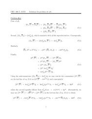
PHY–396 K. Solutions for problem set #2.Problem 1(a):As discussed in class, Euler–Lagrange equations for charged fields can be written in a manifestlycovariant form asD µ∂L∂(D µ φ) − ∂L∂φ= 0. (S.1)In particularly, for φ = Φ, we have∂L∂(D µ Φ) = Dµ Φ ∗ ,∂L∂Φ = −m2 Φ ∗ ,which gives usD µ D µ Φ ∗ + m 2 Φ ∗ = 0. (S.2)Likewise, for φ = Φ ∗ we have∂L∂(D µ Φ ∗ ) = Dµ Φ,∂L∂Φ ∗ = −m2 Φ,and thereforeD µ D µ Φ + m 2 Φ = 0.(S.3)As for the vector fields A ν , the Lagrangian (1) depends on ∂ µ A ν only through F µν , whichgives us the usual Maxwell equation∂ µ F µν = J ν where J ν ≡ − ∂L∂A ν.(S.4)To obtain the current J ν , we notice that the covariant derivatives of the charged fields Φ and1

Φ ∗ depend on the gauge field:∂D µ Φ∂A ν= iqδ ν µΦ,∂D µ Φ ∗∂A ν= −iqδ ν µΦ ∗ . (S.5)Consequently,J ν = − ∂L∂D ν Φ × (iqΦ) −= −iq (ΦD ν Φ ∗ − Φ ∗ D ν Φ) .∂L∂D ν Φ ∗ × (−iqΦ∗ )(S.6)Note that all derivatives on the last line here are gauge-covariant, which makes the currentJ ν gauge invariant. In a non-covariant form,J ν = iqΦ ∗ D ν Φ − iqΦ D ν Φ ∗ − 2q 2 Φ ∗ Φ A ν . (S.7)To prove the conservation of this current, we use the Leibniz rule for covariant derivatives,D ν (XY ) = XD ν Y + Y D ν X. Thus,∂ µ (Φ ∗ D µ Φ) = D µ (Φ ∗ D µ Φ) = (D µ Φ ∗ )(D µ Φ) + Φ ∗ (D µ D µ Φ),∂ µ (ΦD µ Φ ∗ ) = D µ (ΦD µ Φ ∗ ) = (D µ Φ)(D µ Φ ∗ ) + Φ (D µ D µ Φ ∗ ),(S.8)and hence in light of eq. (S.6)for the current,∂νJ ν()= −iq (D ν Φ)(D ν Φ ∗ ) + Φ(D ν D ν Φ ∗ )= iqΦ ∗ D 2 Φ − iqΦ D 2 Φ ∗〈〈by equations of motion〉〉= iqΦ ∗ (−m 2 Φ) − iqΦ(−m 2 Φ ∗ )= 0.()+ iq (D ν Φ ∗ )(D ν Φ) + Φ ∗ (D ν D ν Φ)(S.9)Q.E.D.2

Problem 1(b):According to the Noether theorem,whereT µνNoether=∂L∂(∂ µ A λ ) ∂ν A λ +∂L∂(∂ µ Φ) ∂ν Φ += T µνµνNoether(EM) + TNoether (matter)∂L∂(∂ µ Φ ∗ ) ∂ν Φ ∗− g µν L(S.10)similar to the free EM fields, andT µνNoether (EM) = −F µλ ∂ ν A λ + 1 4 gµν F κλ F κλ (S.11)T µνNoether (matter) = Dµ Φ ∗ ∂ ν Φ + D µ Φ ∂ ν Φ ∗ − g µν( D λ Φ ∗ D λ Φ − m 2 Φ ∗ Φ ) . (S.12)Both terms on the second line of eq. (S.10) lack µ ↔ ν symmetry and gauge invariance andthus need ∂ λ K λµν corrections for some K λµν = −K µλν . We would like to show that the sameK λµν = −F µλ A ν we used to improve the free electromagnetic stress-energy tensor will nowimprove both the T µν µνEMand T mat at the same time!Indeed, to improve the scalar fields’ stress-energy tensor we need∆T µνmatter ≡ T µνµνtrue (matter) − TNoether (matter)= D µ Φ ∗ (D ν Φ − ∂ ν Φ) + D µ Φ(D ν Φ ∗ − ∂ ν Φ ∗ )= D µ Φ ∗ (iqA ν Φ) + D µ Φ(−iqA ν Φ ∗ )(S.13)= −A ν (iqΦ ∗ D µ Φ − iqΦD µ Φ ∗ )= −A ν J µ ,while the improvement of the EM stress-energy requires (cf. previous homework 1.2)∆T µνEM = −F µλ (F ν λ − ∂ν A λ ) = +F µλ ∂λA ν = ∂ λ(−F λµ A ν) + A ν J µ . (S.14)Altogether, to symmetrize the whole stress-energy tensor, we needQ.E.D.(∆T µνtot ≡ T µνµνtrue (total) − TNoether (total) = ∂ λ F µλ A ν ≡ K λµν) .3

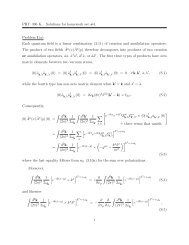
Problem 1(c):Because the fields Φ(x) and Φ ∗ (x) have opposite electric charges, their product is neutral andtherefore ∂ µ (Φ ∗ Φ) = D µ (Φ ∗ Φ) = (D µ Φ ∗ )Φ + Φ ∗ (D µ Φ). Similarly,∂ µ ((D µ Φ ∗ ) (D ν Φ)) = (D µ D µ Φ ∗ ) (D ν Φ) + (D µ Φ ∗ ) (D µ D ν Φ)= −m 2 Φ ∗ (D ν Φ) + (D µ Φ ∗ ) (D ν D µ Φ + iqF µν Φ)(S.15)where we have applied the field equation ( D µ D µ + m 2) Φ ∗ (x) = 0 to the first term on theright hand side and used [D µ , D ν ]Φ = iqF µν Φ to expand the second term. Likewise,∂ µ ((D µ Φ) (D ν Φ ∗ )) = (D µ D µ Φ) (D ν Φ ∗ ) + (D µ Φ) (D µ D ν Φ ∗ )= −m 2 Φ (D ν Φ ∗ ) + (D µ Φ) (D ν D µ Φ ∗ − iqF µν Φ ∗ )(S.16)and∂ µ[−g ( )]µν D λ Φ ∗ D λ Φ − m 2 Φ ∗ Φ( )= −∂ ν D λ Φ ∗ D λ Φ+ m 2 ∂ ν (Φ ∗ Φ)= − (D ν D µ Φ ∗ ) (D µ Φ) − (D µ Φ ∗ ) (D ν D µ Φ)+ m 2 Φ (D ν Φ ∗ ) + m 2 Φ ∗ (D ν Φ) .Together, the left hand sides of eqs. (S.15), (S.16) and (S.17) comprise ∂ µ T µνmat(S.17)— cf. eq. (7).On the other hand, combining the right hand sides of these three equations results in massivecancellation of all terms except those containing the gauge field strength tensor F µν . Thus,∂ µ T µνmat = (D µ Φ ∗ ) (iqF µν Φ) + (D µ Φ) (−iqF µν Φ ∗ )= F µν (iqΦ D µ Φ ∗ − iqΦ ∗ D µ Φ)(S.18)= F µν J ν .And since in the previous homework we have shown ∂ µ T µνEM = −F µν J ν , it follows that thetotal stress tensor (4) is conserved, ∂ µ T µν = 0. Q.E.D.4

Problem 2(a):According to the time-independent Maxwell equations (10), the divergences ∇ · Ê and ∇ · ˆBvanish as operators and therefore should commute with any other operator in the theory. Onthe other hand, the commutation relations of the ∇ · Ê and ∇ · ˆB follow directly from thoseof the Ê and ˆB field themselves:[∇ · Ê(x), whatever(x ′ ) ] = ∂ [Êi ∂x i (x), same whatever(x ′ ) ] ,[∇ · ˆB(x), whatever(x ′ ) ] = ∂ [ ˆBi ∂x i (x), same whatever(x ′ ) ] .(S.19)Thus to make sure that the fields’ commutation relations (11) are consistent with eqs. (10),we must verify that∂∂x i [Êi (x), Êj (x ′ ) ] = 0,∂∂x i [Êi (x), ˆB j (x ′ ) ] = 0,∂∂x i [ ˆBi (x), Êj (x ′ ) ] = 0,∂∂x i [ ˆBi (x), ˆB j (x ′ ) ] = 0,Plugging in the commutation relations (11) into these formulæ, we immediately see that(S.20)∂∂x i [Êi (x), Êj (x ′ ) ] =∂∂x i [ ˆBi (x), ˆB j (x ′ ) ] = 0(S.21)while∂∂x i [Êi (x), ˆB j (x ′ ) ] =∂ (∂x i −i¯hc ɛ ijk∂)∂x k δ(3) (x − x ′ )= 0 (S.22)because ɛ ijk∂∂x i∂∂x k≡ 0. Likewise,∂∂x i [ ˆBi (x), Êj (x ′ ) ] =∂ (∂x i +i¯hc ɛ jik= −i¯hc ɛ jik ∂∂x i∂)∂x ′k δ(3) (x − x ′ )∂∂x k δ(3) (x − x ′ ) = 0.(S.23)Q.E.D.5

Problem 2(b):According to eqs. (11), at equal times [ ˆB i , 1 2 ˆB 2 (x ′ )] = 0 while[ ˆB i , 1 2Ê2 (x ′ )] = Êj (x ′ ) × [ ˆB i (x), Êj (x ′ )] = Êj (x ′ ) × (+i¯hc)ɛ jik ∂∂x ′k δ(3) (x ′ − x),hence∫[ ˆB i (x), Ĥ] = d 3 x ′ (+i¯hc)ɛ jik Ê j (x ′ ) ×∂∂x ′k δ(3) (x ′ − x) = −i¯hc ɛ jik ∇ k Ê j (x),(S.24)(S.25)or in vector notations,[ˆB(x), Ĥ] = −i¯hc ∇ × Ê.(S.26)Consequently, in the Heisenberg picture1c∂∂t ˆB(x, t) = −∇ × Ê(x, t).(12.a)Likewise, [Êi , 1 2Ê2 (x ′ )] = 0 while[Êi , 1 2 ˆB 2 (x ′ )] = ˆB j (x ′ ) × [Êi (x), ˆB j (x ′ )] = ˆB j (x ′ ) × (−i¯hc)ɛ ijk ∂∂x k δ(3) (x ′ − x),hence∫[Êi (x), Ĥ] = d 3 x ′ (−i¯hc)ɛ ijk ˆBj (x ′ ) ×∂∂x k δ(3) (x ′ − x) = −i¯hc ɛ ijk ∇ ˆBj k(x),(S.27)(S.28)or in vector notations,[Ê(x), Ĥ] = +i¯hc ∇ × ˆB.(S.29)Consequently, in the Heisenberg picture1c∂∂t ˆB(x, t) = +∇ × Ê(x, t).(12.b)Q.E.D.6

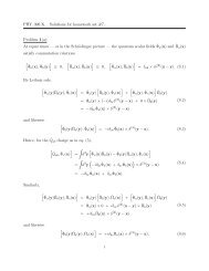
Problem 3(a):In the Hamiltonian formalism for the classical fields Φ(x) and Φ ∗ (x), the canonical conjugatefields areΠ(x) =∂L∂(∂ 0 Φ ∗ ) = ∂ 0Φ(x) and Π ∗ (x) =∂L∂(∂ 0 Φ) = ∂ 0Φ ∗ (x).(S.30)The canonical conjugation implies canonical Poisson brackets between the classical fields Φ(x)and Π ∗ (x), and likewise Φ ∗ (x) and Π(x) and hence the canonical commutation relation betweentheir quantum counterparts: In the Schrödinger picture[ˆΦ(x), ˆΦ(x ′ )] = [ˆΦ(x), ˆΦ † (x ′ )] = [ˆΦ † (x), ˆΦ † (x ′ )] = 0,[ˆΠ(x), ˆΠ(x ′ )] = [ˆΠ(x), ˆΠ † (x ′ )] = [ˆΠ † (x), ˆΠ † (x ′ )] = 0,[ˆΦ(x), ˆΠ(x ′ )] = [ˆΦ † (x), ˆΠ † (x ′ )] = 0,(S.31)[ˆΦ(x), ˆΠ † (x ′ )] = [ˆΦ † (x), ˆΠ(x ′ )] = iδ (3) (x − x ′ ).In the Heisenberg picture, we have similar commutation relations for equal times t = t ′ ; forun-equal times, the formulæ are much more complicated.Classically, the Hamiltonian density isH = Π∂ 0 Φ + Π ∗ ∂ 0 Φ ∗− L= Π ∗ Π + ∇Φ ∗ · ∇Φ + m 2 Φ ∗ Φ,(S.32)so the quantum theory’s Hamiltonian is obviously as in eq. (15).Q.E.D.Problem 3(b):Fourier transforming the canonical commutation relations (S.31) results in[ˆΦ p , ˆΦ p ′] = [ˆΦ p , ˆΦ † p ′ ] = [ˆΦ † p, ˆΦ † p ′ ] = 0,[ˆΠ p , ˆΠ p ′] = [ˆΠ p , ˆΠ † p ′ ] = [ˆΠ † p, ˆΠ † p ′ ] = 0,[ˆΦ p , ˆΠ p ′] = [ˆΦ † p, ˆΠ † p ′ ] = 0,(S.33)[ˆΦ p , ˆΠ † p ′ ] = [ˆΦ † p, ˆΠ p ′] = δ p,p′ .7

Consequently,[â p , â p ′] = [â p , ˆb † p ′ ] = [ˆb † p, ˆb † p ′ ] = 0 (S.34)because all the ˆΦ p and all the ˆΠ p operators commute with each other, and likewise[ˆb p , ˆb p ′] = [ˆb p , â † p ′ ] = [â † p, â † p ′ ] = 0(S.35)because all the ˆΦ † p and all ˆΠ † p operators commute with each other too. Less obviously[â p , ˆb p ′] =12 √ E p E p′= δ p,−p′ × E p ′ − E p2 √ E p E p′(Ep E p ′(0) + iE p (iδ p,−p ′) + iE p ′(−iδ p,−p ′) − (0) )= 0,(S.36)and similarly [â † p, ˆb † p ′ ] = 0. Finally,[â p , â † p ′ ] = [ˆb p , ˆb † p ′ ] =12 √ (E p E p ′(0) − iE p (iδ p,p ′) + iE p ′(−iδ p,p ′) + (0))E p E p′= δ p,p′ × E p ′ + E p2 √ E p E p′= δ p,p′ .(S.37)Q.E.D.Problem 3(c):First, Fourier-transforming the free Hamiltonian (15) gives usĤ free= ∑ p(ˆΠ† p ˆΠp + E 2 p ˆΦ † p ˆΦ p). (S.38)Second, we reverse the definitions (17) to obtainˆΦ p =1√(â p + ˆb)†−p2Epand ˆΠp =√ 2Ep2i(ˆbp − â † −p). (S.39)8

Third, we calculateE 2 p ˆΦ † p ˆΦ p+ ˆΠ −p ˆΠ† −p= E (pâ † p +2ˆb)−p(âp + ˆb)†−p(= E p × â † pâ p + ˆb)−pˆb† −p(= E p × â † pâ p + ˆb † −pˆb −p + 1Finally, we put eqs. (S.40) and (S.38) together and deriveĤ free = ∑ (E 2 ˆΦ p † ˆΦ p p + ˆΠ)−p ˆΠ† −pp= ∑ E p(â † pâ p + ˆb)†−pˆb −p + 1p= ∑ )(E p â † pâ p + E pˆb† pˆbp + const.p+ E (pâ † p −2ˆb)−p(âp − ˆb)†−p)(S.40)(S.41)Q.E.D.Problem 3(d):We begin by Fourier transforming the charge operator∫∫ (ˆQ = d 3 x ˆρ(x) = d 3 x {ˆΠ† i2(x), ˆΦ(x) } − 2{ˆΠ(x), i ˆΦ† (x) }) , (S.42)which yieldsˆQ = ∑ p(i2{ˆΦ† p , ˆΠ}p −i2{ˆΦp , ˆΠ † } )p . (S.43)Next, we re-express the anticommutators here in terms of the creation and annihilator operatorsaccording to eqs. (S.39). After simple algebra we findi2{ˆΦ† p , ˆΠ}p =12(â † pâ p − ˆb)†−pˆb −p + â † pˆb † −p − â pˆb −p−i2,{ˆΦp , ˆΠ † p}=12(â † pâ p − ˆb † −pˆb −p − â † pˆb † −p)+ â pˆb −p ,(S.44)and thereforeˆQ = ∑ p(â † pâ p − ˆb † −pˆb −p)= ∑ p(â † pâ p − ˆb † pˆb p). (21)Q.E.D.9

Problem 3(e):According to eq. (22), classicallyT 0i = ∂ 0 Φ ∗ ∂ i Φ + ∂ 0 Φ ∂ i Φ ∗ = −Π ∗ ∂ i Φ − Π ∂ i Φ ∗ , (S.45)and hence in the quantum theory∫ˆP mech = d 3 x(− 1 2{ˆΠ† , ∇ˆΦ } − 1 2{ˆΠ, ∇ˆΦ† }) . (S.46)Fourier-transforming this formula, we arrive atˆP mech= ∑ p(− ip 2{ˆΠ† p , ˆΦ} ipp +{ˆΠp ,2ˆΦ † } )p , (S.47)and hence in light of eqs. (S.44),ˆP mech= ∑ p(p â † pâ p − p ˆb † −pˆb −p)= ∑ p(p â † pâ p + p ˆb † pˆb p). (23)Q.E.D.10