Alain Connes (pdf)

NONCOMMUTATIVE GEOMETRY
Alain Connes
As long as we consider geometry as intimately related to our model of space-time, Einstein’s
general relativity clearly vindicated the ideas of Gauss and Riemann, allowing
for variable curvature. They formulated the intrinsic geometry of a curved space independently
of its embedding in Euclidean space. The two key notions are those of
manifold of arbitrary dimension, whose points are labelled by finitely many real numbers
x µ , and that of the line element i.e. the infinitesimal unit of length which, when
carried around, allows to measure distances. The infinitesimal calculus allows to encode
the geometry by the formula for the line element ds in local terms
ds 2 = g µν dx µ dx ν . (1)
and to generalise most of the concepts which were present either in euclidean or noneuclidean
geometry while considerably enhancing the number of available interesting examples.
In particular the idea of straight line does continue to make sense and is given
by the equation of geodesics,
d 2 x µ
dt 2
= − 1 2 gµα (g αν,ρ + g αρ,ν − g νρ,α ) dxν
dt
which, when applied in the modified Minkowski Lorentzian metric,
dx ρ
dt
(2)
dx 2 + dy 2 + dz 2 − (1 + 2V (x, y, z)) dt 2 (3)
gives Newton’s law for the motion in the gravitational field deriving from the potential
function V .
Riemann was sufficiently cautious in his lecture on the foundation of geometry to question
the validity of his hypotheses in the infinitely small. He explicitly proposed to
”gradually modify the foundations under the compulsion of facts which cannot be explained
by it” in case physics would find new unexplained phenomena in the exploration
of smaller scales.
The origin of noncommutative geometry can be traced back to the discovery of such
unexplained phenomena in the phase space of the microscopic mechanical system describing
an atom. This system manifests itself through its interaction with radiation
1

and the basic laws of spectroscopy, as found in particular by Ritz and Rydberg, are in
contradiction with the ”manifold” picture of the phase space.
The very bare fact which came directly from experimental findings in spectroscopy and
was unveiled by Heisenberg (and then understood at a more mathematical level by Born,
Jordan, Dirac and the physicists of the late 1920’s) is that whereas when you are dealing
with a manifold you can parametrize (locally) its points x by real numbers x 1 , x 2 , . . .
which specify completely the situation of the system, when you turn to the phase space
of a microscopic mechanical system, even of the simplest kind, the coordinates, namely
the real numbers x 1 , x 2 , . . . that you would like to use to parametrize points, actually
do not commute.
This means that the classical geometrical framework is too narrow to describe in a
faithful manner many physical spaces of great interest. In noncommutative geometry
one replaces the usual notion of manifold formed of points labelled by coordinates
with spaces of a more general nature (as we shall see later). Usual geometry is just
a particular case of this new theory, in the same way as Euclidean and non Eulidean
geometry are particular cases of Riemannian geometry. Many of the familar geometrical
concepts do survive in the new theory, but they carry also a new unexpected meaning.
Before describing the novel notion of space it is worthwile to explain in simple terms
how noncommutative geometry modifies the measurement of distances. Such a simple
description is possible because the evolution between the Riemannian way of measuring
distances and the new (noncommutative) way exactly parallels the improvement of
the standard of length ∗ in the metric system. The original definition of the meter at
the end of the 18th century was based on a small portion (one forty millionth part)
of the size of the largest available macroscopic object (here the earth circonference).
Moreover this “unit of length” became concretely represented in 1799 as “metre des
archives” by a platinum bar localised near Paris. The international prototype was a
more stable copy of the “metre des archives” which served to define the meter. The
most drastic change in the definition of the meter occured in 1960 when it was redefined
as a multiple of the wavelength of a certain orange spectral line in the light emitted
by isotope 86 of the krypton. This definition was then replaced in 1983 by the current
definition which using the speed of light as a conversion factor is expressed in terms of
inverse-frequencies rather than wavelength, and is based on a hyperfine transition in
the caesium atom. The advantages of the new standard are obvious. No comparison to
a localised “metre des archives” is necessary, the uncertainties are estimated as 10 −15
and for most applications a commercial caesium beam is sufficiently accurate. Also we
could (if any communication were possible) communicate our choice of unit of length to
aliens, and uniformise length units in the galaxy without having to send out material
copies of the “metre des archives”!
As we shall see below the concept of “metric” in noncommutative geometry is precisely
based on such a spectral data.
Let us now come to “spaces”. What the discovery of Heisenberg showed is that the
familiar duality of algebraic geometry between a space and its algebra of coordinates
(i.e. the algebra of functions on that space) is too restrictive to model the phase space
of microscopic physical systems. The basic idea then, is to stretch this duality so
that the algebra of coordinates on a space, is no longer required to be commutative.
Gelfand’s work on C ∗ -algebra provides the right framework to define noncommutative
∗ or equivalently of time using the speed of light as a conversion factor
2

topological spaces. They are given by their algebra of continuous functions which can
be an arbitrary, not necessarily commutative C ∗ -algebra.
It turns out that there is a wealth of examples of spaces which have obvious geometric
meaning but which are best described by a noncommutative algebra of coordinates.
The first examples came, as we saw above, from phase space in quantum mechanics
but there are many others, such as the leaf spaces of foliations, the duals of nonabelian
discrete groups, the space of Penrose tilings, the noncommutative torus which plays a
role in M-theory compactification, the Brillouin zone in solid state physics, the spaces
underlying ”quantum groups” obtained as deformations of classical Lie groups and
finally the space of Q-lattices which is a natural geometric space with an action of
the scaling group providing a spectral interpretation of the zeros of the L-functions
of number theory and an interpretation of the Riemann explicit formulas as a trace
formula.
The second vital ingredient of the theory is the extension of geometric ideas to the
noncommutative framework. The stretching of geometric thinking imposed by passing
to noncommutative spaces forces one to rethink about most of our familiar notions.
The difficulty is not to add arbitrarily the adjective quantum to our familiar geometric
language but to develop far reaching extensions of classical concepts. As we shall see
below this has been achieved with variable degrees of perfection for measure theory,
topology, differential geometry, and Riemannian geometry.
Let us first describe the basic principle which allows to establish the general duality,
Quotient spaces ↔ Noncommutative algebra . (4)
Many of the spaces that we are used to consider are not really described by listing their
points but are obtained by identifications, their elements being given as equivalence
classes in a larger space M.
There are two ways of proceeding at the algebraic level in order to identify two points
a and b in a given space M. The first way is to consider only those functions f on M
which take the same value at the points a and b, namely that satisfy f(a) = f(b). Thus
the usual algebra of functions associated to the quotient is
A = {f; f(a) = f(b)} . (5)
There is however another way of performing, in an algebraic manner, the above quotient
operation. It consists, instead of taking the subalgebra given by (5), to adjoin to the
algebra of functions the identification of a with b. The obtained algebra is, restricting
to M = {a, b}, the algebra of two by two matrices
B =
{
f =
[ ]}
faa f ab
. (6)
f ba f bb
In other words we do not require that functions have the same value at a and b, but we
allow the two points a and b to relate to each other via the off-diagonal matrix elements
f a b and f b a . The effect of these off-diagonal matrix elements is to identify these two
points into one point in the spectrum of the algebra, i. e. in the space of its irreducible
representations. Indeed the irreducible representation corresponding to a (associated
to the pure state a) has now become equivalent to the representation coming from b.
3

Now in this very simple example of two points, the two different algebras that one
obtains are still equivalent. The equivalence between A and B is called Morita equivalence
[28] and means that the corresponding categories of right modules are equivalent.
There is of course an obvious difference between A and B since, unlike A, the algebra
B is no longer commutative.
Let me now give another simple example, in which the two ways of doing things do not
give the same answer, even up to Morita equivalence. We take two intervals, [0,1], and
we want to identify the insides of these two intervals but not their endpoints.
Applying the first procedure above, and working in the smooth (C ∞ ) category, we
obtain the algebra of smooth functions on M = [0, 1]× {0, 1} which have equal values
on the points (x, 0) and (x, 1) for any x in the open interval ]0, 1[. But, by continuity,
functions which are equal inside the intervals are also equal at the endpoints. Thus
what we get is simply the algebra A = C ∞ ([0, 1]), whose spectrum is the interval [0, 1],
and we did not succeed to keep the endpoints apart.
Applying the second procedure, we get the algebra of smooth maps from the interval
[0,1] to 2 × 2 matrices, but since the endpoints are not identified with each other, we
only get smooth maps which have diagonal matrices as boundary values. The obtained
algebra B is quite interesting, it is the smooth group ring of the dihedral group, namely
of the free product of two groups with 2 elements. This algebra is quite different from
the first one, and certainly not Morita equivalent to C ∞ ([0, 1]).
In general, when we consider arbitrary quotient spaces, the two algebras A and B are
not Morita equivalent. The first operation (5) is of a cohomological flavor while the
second (6) keeps a closer contact with the quotient space.
We shall now describe a basic concrete example, the noncommutative torus whose
noncommutative differential geometry was unveiled in 1980 ([8]). This example is the
following: consider the 2-torus
M = R 2 /Z 2 . (7)
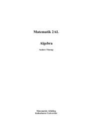
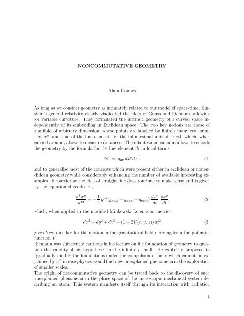
The space X which we contemplate is the space of solutions of the differential equation,
where θ ∈]0, 1[ is a fixed irrational number (fig 1).
dx = θdy x, y ∈ R/Z (8)
1
θ
y
dx = θdy
x, y ∈ R/Z
0
x 1
Figure 1
Thus the space we are interested in here is just the space of leaves of the foliation defined
by the differential equation. We can label such a leaf by a point of the transversal given
by y = 0 which is a circle S 1 = R/Z, but clearly two points of the transversal which
differ by an integer multiple of θ give rise to the same leaf. Thus
X = S 1 /θZ (9)
4

i.e. X is the quotient of S 1 by the equivalence relation which identifies any two points
on the orbits of the irrational rotation
R θ x = x + θ mod 1 . (10)
When we deal with S 1 as a space in the various categories (smooth, topological, measurable)
it is perfectly described by the corresponding algebra of functions,
C ∞ (S 1 ) ⊂ C(S 1 ) ⊂ L ∞ (S 1 ) . (11)
When one applies the operation (5) to pass to the quotient, one finds, irrespective of
which category one works with, the trivial answer
A = C . (12)
The operation (6) however gives very interesting algebras, by no means Morita equivalent
to C. In the above situation of a quotient by a group action the operation (6) is
the construction of the crossed product familiar to algebraist from the theory of central
simple algebras.
An element of B is given by a power series
b = ∑ n∈Z
b n U n (13)
where each b n is an element of the algebra (11), while the multiplication rule is given
by
UhU −1 = h ◦ R −1
θ
. (14)
Now the algebra (11) is generated by the function V on S 1 ,
V (α) = exp(2πiα) α ∈ S 1 (15)
and it follows that B admits the generating system (U, V ) with presentation given by
the relation
UV U −1 = λ −1 V λ = exp2πiθ . (16)
Thus, if for instance we work in the smooth category a generic element b of B is given
by a power series
b = ∑ Z 2 b nm U n V m , b ∈ S(Z 2 ) (17)
where S(Z 2 ) is the Schwartz space of sequences of rapid decay on Z 2 .
This algebra has a very rich and interesting algebraic structure. It is (canonically up
to Morita equivalence) associated to the foliation (8) and the interplay between the
geometry of the foliation and the algebraic structure of B begins by noticing that to
a closed transversal of the foliation corresponds canonically a finite projective module
over B.
From the transversal x = 0, one obtains the following right module over B. The
underlying linear space is the usual Schwartz space,
S(R) = {ξ, ξ(s) ∈ C ∀s ∈ R} (18)
of smooth functions on the real line all of whose derivatives are of rapid decay.
5

The right module structure is given by the action of the generators U, V
(ξU)(s) = ξ(s + θ) , (ξV )(s) = e 2πis ξ(s) ∀s ∈ R . (19)
One of course checks the relation (16), and it is a beautiful fact that as a right module
over B the space S(R) is finitely generated and projective (i.e. complements to a free
module). It follows that it has the correct algebraic atributes to deserve the name of
“noncommutative vector bundle” according to the dictionary,
Space
Vector bundle
Algebra
Finite projective module.
The concrete description of the general finite projective modules over A θ is obtained
by combining the results of [8] [27] [29]. They are classified up to isomorphism by a
pair of integers (p, q) such that p + q θ ≥ 0 and the corresponding modules H θ p,q are
obtained by the above construction from the transversals given by closed geodesics of
the torus M.
The algebraic counterpart of a vector bundle is its space of smooth sections C ∞ (X, E)
and one can in particular compute its dimension by computing the trace of the identity
endomorphism of E. If one applies this method in the above noncommutative example,
one finds
dim B (S) = θ . (20)
The appearance of non integral dimension is very exciting and displays a basic feature
of von Neumann algebras of type II. The dimension of a vector bundle is the only
invariant that remains when one looks from the measure theoretic point of view (i.e.
when one takes the third algebra in (11)). The von Neumann algebra which describes
the quotient space X from the measure theoretic point of view is the crossed product,
R = L ∞ (S 1 ) >✁ Rθ Z (21)
and is the well known hyperfinite factor of type II 1 . In particular the classification of
finite projective modules E over R is given by a positive real number, the Murray and
von Neumann dimension,
dim R (E) ∈ R + . (22)
The next surprise is that even though the dimension of the above module is irrational,
when we compute the analogue of the first Chern class, i.e. of the integral of the
curvature of the vector bundle, we obtain an integer. Indeed the two commuting vector
fields which span the tangent space for an ordinary (commutative) 2-torus correspond
algebraically to two commuting derivations of the algebra of smooth functions. These
derivations continue to make sense when the generators U and V of C ∞ (T 2 ) no longer
commute but satisfy (16) so that they generate C ∞ (T 2 θ ). They are given by the same
formulas as in the commutative case,
δ 1 = 2πiU
∂
∂U , δ 2 = 2πiV
so that δ 1 ( ∑ b nm U n V m ) = 2πi ∑ nb nm U n V m and similarly for δ 2 . One still has of
course
δ 1 δ 2 = δ 2 δ 1 (24)
∂
∂V
(23)
6

and the δ j are still derivations of the algebra B = C ∞ (T 2 θ ),
δ j (bb ′ ) = δ j (b)b ′ + bδ j (b ′ ) ∀b, b ′ ∈ B . (25)
The analogues of the notions of connection and curvature of vector bundles are straightforward
to obtain since a connection is just given by the associated covariant differentiation
∇ on the space of smooth sections. Thus here it is given by a pair of linear
operators,
∇ j : S(R) → S(R) (26)
such that
∇ j (ξb) = (∇ j ξ)b + ξδ j (b) ∀ξ ∈ S , b ∈ B . (27)
One checks that, as in the usual case, the trace of the curvature Ω = ∇ 1 ∇ 2 − ∇ 2 ∇ 1 , is
independent of the choice of the connection. Now the remarkable fact here ([8]) is that
(up to the correct powers of 2πi) the integral curvature of S is an integer. In fact for
the following choice of connection the curvature Ω is constant, equal to 1 so that the
θ
irrational number θ disappears in the integral curvature, θ × 1 θ
(∇ 1 ξ)(s) = − 2πis
θ
ξ(s) (∇ 2 ξ)(s) = ξ ′ (s) . (28)
With this integrality, one could get the wrong impression that the algebra B = C ∞ (T 2 θ )
looks very similar to the algebra C ∞ (T 2 ) of smooth functions on the 2-torus. A striking
difference is obtained by looking at the range of Morse functions. The range of a Morse
function on T 2 is of course a connected interval. For the above noncommutative torus
T 2 θ the range of a Morse function is the spectrum of a real valued function such as
h = U + U ∗ + µ(V + V ∗ ) (29)
and it can be a Cantor set, i.e. have infinitely many disconnected pieces. This shows
that the one dimensional shadows of our space T 2 θ are truly different from what they are
in the commutative case. The above noncommutative torus T 2 θ is the simplest example
of noncommutative manifold, it arises naturally not only from foliations but also from
the Brillouin zone in the Quantum Hall effect as understood by J. Bellissard, and in M-
theory as we shall see next. Indeed both the noncommutative tori and the components
∇ j of the Yang-Mills connections occur naturally in the classification of the BPS states
in M-theory [15]. In the matrix formulation of M-theory the basic equations to obtain
periodicity of two of the basic coordinates X i turn out to be the following
U i X j Ui −1 = X j + a δ j i , i = 1, 2 (30)
where the U i are unitary gauge transformations.
The multiplicative commutator U 1 U 2 U1 −1 U2 −1 is then central and in the irreducible case
its scalar value λ = exp 2πiθ brings in the algebra of coordinates on the noncommutative
torus. The X j are then the components of the Yang-Mills connections. It is quite
remarkable that the same picture emerged from the other information one has about M-
theory concerning its relation with 11 dimensional supergravity and that string theory
dualities could be interpreted using Morita equivalence. The latter [28] relates the
values of θ on an orbit of SL(2, Z) and this type of relation, which is obvious from the
foliation point of view, would be invisible in a purely deformation theoretic perturbative
expansion like the one given by the Moyal product.
7

We shall come back later to the natural moduli space for the noncommutative tori
and to the metric aspect when we have the correct general tools. But we first need to
dispell the impression that the noncommutative torus, because of its ubiquity, is the
only example of noncommutative space.
A very large class of examples is provided first of all by the duals of discrete groups. We
saw already the dual of the dihedral group which was truly very simple, but as soon as
one considers more complicated discrete groups one finds that their duals are exactly
like leaf spaces of foliations. It is important to understand at least on one example why
the dual of a discrete non abelian group is in essence a quotient space, like the one we
analysed above for foliations. Thus, let Γ be the solvable group Γ = Z 2 >✁ α Z obtained
as the semi-direct product of the additive group Z 2 by the action of Z given by the
matrix
[ ]
1 1
T = ∈ SL(2, Z) . (31)
1 2
By Mackey’s theory of induced representations each element x of the 2-torus Ẑ2 which
is the Pontrjagin dual of the group Z 2 , determines by induction an irreducible representation
of Γ,
π x ∈ Irrep(Γ) . (32)
Moreover the two representations π x and π y associated to x, y ∈ Ẑ2 , are equivalent iff
x and y are on the same orbit of the (transposed) transformation T of Ẑ2 . One does
not get all irreducible representations of Γ by this procedure but the quotient space
X = Ẑ2 / ∼ , x ∼ y iff y = T n x for some n (33)
does correspond in the above sense to the smooth group ring of Γ.
Here is a more complete list of basic examples,
Space of leaves of foliations
Space of irreducible representations of discrete groups
Space of Penrose tilings of the plane
Brillouin zone in the quantum Hall effect
Phase space in quantum mechanics
Space time
Another rich class of examples arises from deformation theory such as deformation of
Poisson manifolds, quantum groups and their homogeneous spaces.
Let me finally mention the space of Adele classes, a noncommutative space whose
understanding is intimately related to the location of the zeros of Hecke L-functions in
the number field case.
Thus there is no shortage of examples of noncommutative spaces that beg our understanding
but which are very difficult to comprehend.
The reason why I started working in noncommutative geometry is that I found that
even at the very coarse level of measure theory, the general noncommutative case was
becoming highly non trivial. When you look at an ordinary space and you do measure
theory, you use the Lebesgue theory which is a beautiful theory, but all spaces are the
same, there is nothing really happening as far as classification is concerned. This is
not at all the case in noncommutative measure theory. What happens there is very
surprising. It is an absolutely fascinating fact that when you take a non commutative
algebra M from the measure theory point of view, such an algebra evolves with time !
8

What I mean is that it admits a god-given time evolution given by a canonical group
homomorphism, ([6])
δ : R → Out(M) = Aut(M)/Int(M) (34)
from the additive group R to the center of the group of automorphism classes of M
modulo inner automorphisms.
This homomorphism is provided by the uniqueness of the, a priori state dependent,
modular automorphism group of a state. Together with the earlier work of Powers,
Araki-Woods and Krieger it was the beginning of a long story which eventually led to the
complete classification ([6], [31], [26], [21], [7], [22]) of approximately finite dimensional
factors (also called hyperfinite).
They are classified by their module,
Mod(M) ⊂
∼
R ∗ + , (35)
which is a virtual closed subgroup of R ∗ + in the sense of G. Mackey, i.e. an ergodic
action of R ∗ + .
One can interpret this classification as a non-trivial Brauer theory for Archimedian
local fields. Local class field theory is interesting and non trivial for local fields which
are non archimedian, like p-adic numbers because such fields K are very far from being
algebraically closed.
But there is nothing comparable when you look at class field over complex numbers,
because the field of complex numbers is algebraically closed, so there is apparently
nothing going on. Now it turns out that the theory of factors gives a non-trivial
replacement for the missing Brauer theory at archimedian places. This can be seen
as follows. To say that a field is algebraically closed can be formulated in terms of
representation theory. It is equivalent to say that when we look at representations
of semisimple objects (groups, algebras...) over this field any such representation can
be decomposed in direct sums of multiples of representations whose commutant is the
scalars. Of course this does hold when we take finite dimensional representations over
C. But as soon as we take infinite dimensional representations a new phenomenon
occurs and it is in perfect analogy with the unramified extensions of p-adic fields.
Non trivial factors occur, they are commutants of representations in Hilbert space and
though they have trivial center, they are not Morita equivalent to C. As we saw these
factors have an invariant, which is called their module, very analogous to the module
of central simple algebras over local fields; this module is not really a subgroup of R ∗ + ,
it’s a virtual subgroup of R ∗ + in the sense that it is a flow. And for factors which are
approximately finite dimensional this flow turns out to give exactly a complete invariant
of factors and all flows occur. This analogy goes quite far, noncommutative manifolds
give examples of construction of the hyperfinite II 1 factor as the crossed product of the
field K q of elliptic functions by a subgroup of its Galois group in perfect analogy with the
Brauer theory. The occurence of the type III 1 factor from simple adelic constructions
yields a spectral interpretation of the zeros of L-functions in number theory ([13]).
So, we see that noncommutative measure theory is already highly non trivial, and
thus we have all reasons to believe that if one goes further in the natural hierarchy of
features of a space, one will discover really interesting new phenomenas.
Measure theory is indeed a very coarse way of looking at a space, and a finer and finer
picture is obtained by going up in the following hierarchy of points of view:
9

Riemannian geometry
Differential geometry
Topology
Measure theory
The development of the topological ideas was prompted by the work of Israel Gel’fand,
whose C* algebras give the required framework for noncommutative topology. The
two main driving forces were the Novikov conjecture on homotopy invariance of higher
signatures of ordinary manifolds as well as the Atiyah-Singer Index theorem. It has
led, through the work of Atiyah, Singer, Brown, Douglas, Fillmore, Miscenko and Kasparov
([1] [3] [25]) to the recognition that not only the Atiyah-Hirzebruch K-theory but
more importantly the dual K-homology admit Hilbert space techniques and functional
analysis as their natural framework. The cycles in the K-homology group K ∗ (X) of a
compact space X are indeed given by Fredholm representations of the C* algebra A of
continuous functions on X. The central tool is the Kasparov bivariant K-theory. A basic
example of C* algebra to which the theory applies is the group ring of a discrete group
and restricting oneself to commutative algebras is an obviously undesirable assumption.
For a C ∗ algebra A, let K 0 (A), K 1 (A) be its K theory groups. Thus K 0 (A) is the
algebraic K 0 theory of the ring A and K 1 (A) is the algebraic K 0 theory of the ring
A ⊗ C 0 (R) = C 0 (R, A). If A → B is a morphism of C ∗ algebras, then there are induced
homomorphisms of abelian groups K i (A) → K i (B). Bott periodicity provides a six
term K theory exact sequence for each exact sequence 0 → J → A → B → 0 of C ∗
algebras and excision shows that the K groups involved in the exact sequence only
depend on the respective C ∗ algebras.
Discrete groups, Lie groups, group actions and foliations give rise through their convolution
algebra to a canonical C ∗ algebra, and hence to K theory groups. The analytical
meaning of these K theory groups is clear as a receptacle for indices of elliptic operators.
However, these groups are difficult to compute. For instance, in the case of
semi-simple Lie groups the free abelian group with one generator for each irreducible
discrete series representation is contained in K 0 Cr ∗G where C∗ r G is the reduced C∗ algebra
of G. Thus an explicit determination of the K theory in this case in particular
involves an enumeration of the discrete series.
We introduced with P. Baum ([2]) a geometrically defined K theory which specializes
to discrete groups, Lie groups, group actions, and foliations. Its main features are
its computability and the simplicity of its definition. In the case of semi-simple Lie
groups it elucidates the role of the homogeneous space G/K (K the maximal compact
subgroup of G) in the Atiyah-Schmid geometric construction of the discrete series.
Using elliptic operators we constructed a natural map µ from our geometrically defined
K theory groups to the above analytic (i.e. C ∗ algebra) K theory groups. Much
progress has been made in the past years to determine the range of validity of the
isomorphism between the geometrically defined K theory groups and the above analytic
(i.e. C ∗ algebra) K theory groups. We refer to the three Bourbaki seminars ([30]) for
an update on this topic and for a precise account of the various contributions. Among
the most important contributions are those of Kasparov and Higson who showed that
the conjectured isomorphism holds for amenable groups. It also holds for real semisimple
Lie groups thanks in particular to the work of A. Wassermann. Moreover the
recent work of V. Lafforgue crossed the barrier of property T, showing that it holds
for cocompact subgroups of rank one Lie groups and also of SL(3, R) or of p-adic
10

Lie groups. He also gave the first general conceptual proof of the isomorphism for
real or p-adic semi-simple Lie groups. The proof of the isomorphism for all connected
locally compact groups, based on Lafforgue’s work has been obtained by J. Chabert,
S. Echterhoff and R. Nest ([5]). The proof by G. Yu of the analogue (due to J. Roe) of
the conjecture in the context of coarse geometry for metric speces which are uniformly
embeddable in hilbert space, and the work of G. Skandalis J. L. Tu, J. Roe and N.
Higson on the groupoid case got very striking consequences such as the injectivity
of the map µ for exact Cr ∗ (Γ) due to Kaminker, Guentner and Ozawa. Finally the
independent results of Lafforgue and Mineyev-Yu show that the conjecture holds for
arbitrary hyperbolic groups (most of which have property T), and P. Julg was even
able to prove the conjecture with coefficients for rank one groups which is probably the
strongest existing positive result. Its possible extension to arbitrary hyperbolic groups
is under intense investigation. On the negative side, recent progress due to Gromov,
Higson, Lafforgue and Skandalis gives counterexamples to the general conjecture for
locally compact groupoids for the simple reason that the functor G → K 0 (Cr ∗ (G)) is
not half exact, unlike the functor given by the geometric group. This makes the general
problem of computing K(Cr ∗ (G)) really interesting. It shows that besides determining
the large class of locally compact groups for which the original conjecture is valid,
one should understand how to take homological algebra into account to deal with the
correct general formulation.
The development of differential geometric ideas, including de Rham homology, connections
and curvature of vector bundles, etc... took place during the eighties thanks to
cyclic cohomology ([10] [9] [32]). This led for instance to the proof of the Novikov conjecture
for hyperbolic groups [17], but got many other applications. Basically, by extending
the Chern-Weil characteristic classes to the general framework it allows for many
concrete computations of differential geometric nature on noncommutative spaces. It
also showed the depth of the relation between the above classification of factors and
the geometry of foliations. For instance, using cyclic cohomology together with the
following simple fact,
“A connected group can only act trivially on a homotopy
invariant cohomology theory”,
(36)
one proves (cf. [11]) that for any codimension one foliation F of a compact manifold V
with non vanishing Godbillon-Vey class one has,
Mod(M) has finite covolume in R ∗ + , (37)
where M = L ∞ (V, F ) and a virtual subgroup of finite covolume is a flow with a finite
invariant measure.
In order to understand what cyclic cohomology is about, it is worthwile to start by
proving , as an exercice, the following simple fact:
”Let A be an algebra and ϕ a trilinear form on A such that 1) ϕ(a 0 , a 1 , a 2 ) =
ϕ(a 1 , a 2 , a 0 ) ∀a j ∈ A. 2) ϕ(a 0 a 1 , a 2 , a 3 )−ϕ(a 0 , a 1 a 2 , a 3 )+ϕ(a 0 , a 1 , a 2 a 3 )−ϕ(a 2 a 0 , a 1 , a 2 ) =
0 ∀a j ∈ A. Then the scalar ϕ n (E, E, E) is invariant under homotopy for projectors
(idempotents) E ∈ M n (A)”
(here ϕ has been uniquely extended to M n (A) using the trace on M n (C), i.e. ϕ n =
ϕ ⊗ Trace).
11

This fact is not difficult to prove, the point is that a deformation of idempotents is
always isospectral,
Ė = [X, E] for some X ∈ M n (A) . (38)
When we take A = C ∞ (M) for a manifold M and let
ϕ(f 0 , f 1 , f 2 ) = 〈C, f 0 df 1 ∧ df 2 〉 ∀f j ∈ A (39)
where C is a 2-dimensional closed de Rham current, the invariant given by the lemma
is equal to (up to normalisation)
〈C, c 1 (E)〉 (40)
where c 1 is the first chern class of the vector bundle E on M whose fiber at x ∈ M
is the range of E(x) ∈ M n (C). In this example we see that for any permutation of
{0, 1, 2} one has:
ϕ(f σ(0) , f σ(1) , f σ(2) ) = ε(σ)ϕ(f 0 , f 1 , f 2 ) (41)
where ε(σ) is the signature of the permutation. However when we extend ϕ to M n (A)
as ϕ n = ϕ ⊗ Tr,
ϕ n (f 0 ⊗ µ 0 , f 1 ⊗ µ 1 , f 2 ⊗ µ 2 ) = ϕ(f 0 , f 1 , f 2 )Tr(µ 0 µ 1 µ 2 ) (42)
the property 41 only survives for cyclic permutations. This is at the origin of the name,
cyclic cohomology, given to the corresponding cohomology theory.
In the example of the noncommutative torus, the cyclic cocycle that was giving an
integral invariant is
where τ is the unique trace,
ϕ(b 0 , b 1 , b 2 ) = τ(b 0 (δ 1 (b 1 )δ 2 (b 2 ) − δ 2 (b 1 )δ 1 (b 2 )) (43)
τ(b) = b 00 for b = ∑ b nm U n W m . (44)
The pairing given by the lemma then gives the Hall conductivity when applied to
a spectral projection of the Hamiltonian (see [12] for an account of the work of J.
Bellissard).
We then obtain in general the beginning of a dictionary relating usual geometrical
notions to their algebraic counterpart in such a way that the latter is meaningfull in
the general noncommutative situation.
Space
Vector bundle
Differential form
DeRham current
DeRham homology
Chern Weil theory
Algebra
Finite projective module
(Class of) Hochschild cycle
(Class of) Hochschild cocycle
Cyclic cohomology
Pairing 〈K(A), HC(A)〉
12

Of course such a dictionary that translates standard notions of geometry in terms
which do not involve commutativity, only gives a superficial idea of noncommutative
geometry, because as we already saw with measure theory, what matters is not only to
translate, but to uncover completely new phenomenas.
For instance, unlike the de Rham cohomology, its noncommutative replacement which
is cyclic cohomology is not graded but filtered. Also it inherits from the Chern character
map a natural integral lattice. These two features play a basic role in the description
of the natural moduli space (or more precisely, its covering Teichmüller space, together
with a natural action of SL(2, Z) on this space) for the noncommutative tori T 2 θ . The
discussion parallels the description of the moduli space of elliptic curves, but involves
the even cohomology instead of the odd one ([15]).
We shall now come to the central notion of noncommutative geometry i.e. the identification
of the noncommutative analogue of the two basic concepts in Riemann’s
formulation of Geometry, namely those of manifold and of infinitesimal line element.
Both of these noncommutative analogues are of spectral nature and combine to give rise
to the notion of spectral triple and spectral manifold, which will be described below.
We shall first describe an operator theoretic framework for the calculus of infinitesimals
which will provide a natural home for the infinitesimal line element ds.
The stage is provided by quantum mechanics. Let us look at the first two lines of the
following dictionary which translates classical notions into the language of operators in
the Hilbert space H:
Complex variable
Operator in H
Real variable
Infinitesimal
Selfadjoint operator
Compact operator
Infinitesimal of order α Compact operator with characteristic values
µ n ∫
satisfying µ n = O(n −α ) , n → ∞
Integral of an infinitesimal
− T = Coefficient of logarithmic
of order 1 divergence in the trace of T .
A variable (in the intuitive sense) should be thought of as an operator in Hilbert space.
The set of values of the variable is the spectrum of the operator, and the number of
times a value is reached is the spectral multiplicity. A real variable corresponds to
a self-adjoint operator. Its spectrum is real and we can act on it by any measurable
function. In general one can act on complex variables only by holomorphic functions,
and this is exactly what happens for non-selfadjoint operators. Now there is in this
dictionary a perfect place for infinitesimals, namely for something which is smaller than
ɛ for any ɛ, without being zero. Of course requiring that the operator norm is smaller
than ɛ for any ɛ, is too strong, but one can be more subtle and ask that for any ɛ positive
one can condition the operator by a finite number of linear conditions, so that its norm
becomes less than ɛ. This is a well known characterization of compact operators in
Hilbert space and they are the obvious candidates for infinitesimals. The basic rules
of infinitesimals are easy to check, for instance the sum of two compact operators is
compact, the product compact times bounded is compact.
The size of the infinitesimal T ∈ K is governed by the rate of decay of the decreasing
sequence of its characteristic values µ n = µ n (T ) as n → ∞. In particular, for all real
13

positive α the following condition defines infinitesimals of order α:
µ n (T ) = O(n −α ) when n → ∞ (45)
(i.e. there exists C > 0 such that µ n (T ) ≤ Cn −α
also form a two–sided ideal and moreover,
∀ n ≥ 1). Infinitesimals of order α
T j of order α j ⇒ T 1 T 2 of order α 1 + α 2 . (46)
Since the size of an infinitesimal is measured by the sequence µ n → 0 it might seem
that one does not need the operator formalism at all, and that it would be enough to
replace the ideal K in L(H) by the ideal c 0 (N) of sequences converging to zero in the
algebra l ∞ (N) of bounded sequences. A variable would just be a bounded sequence, and
an infinitesimal a sequence µ n , µ n → 0. However, this commutative version does not
allow for the existence of variables with range a continuum since all elements of l ∞ (N)
have a point spectrum and a discrete spectral measure. Thus, this is obviously wrong,
because then you exclude variables which have Lebesgue spectrum. It turns out that
it is only because of non commutativity that infinitesimals can coexist with continuous
variables. As we shall see shortly, it is precisely this lack of commutativity between
the line element and the coordinates on a space that will provide the measurement of
distances.
Another key new ingredient in this dictionary is the integral − ∫ which is obtained by the
following analysis, mainly due to Dixmier, of the logarithmic divergence of the partial
traces
Trace N (T ) =
N−1
∑
0
µ n (T ) , T ≥ 0 . (47)
(In fact, it is useful to define Trace Λ (T ) for any positive real Λ > 0 by piecewise affine
interpolation for noninteger Λ).
Define for all order 1 operators T ≥ 0
τ Λ (T ) = 1
log Λ
∫ Λ
e
Trace µ (T )
log µ
dµ
µ
(48)
which is the Cesaro mean of the function Traceµ(T )
log µ
over the scaling group R ∗ + .
For T ≥ 0, an infinitesimal of order 1, one has
Trace Λ (T ) ≤ C log Λ (49)
so that τ Λ (T ) is bounded. The essential property is the following asymptotic additivity
of the coefficient τ Λ (T ) of the logarithmic divergence (49):
|τ Λ (T 1 + T 2 ) − τ Λ (T 1 ) − τ Λ (T 2 )| ≤ 3C
log(log Λ)
log Λ
(50)
for T j ≥ 0.
An easy consequence of (50) is that any limit point τ of the nonlinear functionals τ Λ
for Λ → ∞ defines a positive and linear trace on the two–sided ideal of infinitesimals
of order 1,
14

In practice the choice of the limit point τ is irrelevant because in all important examples
T is a measurable operator, i.e.:
τ Λ (T ) converges when Λ → ∞ . (51)
Thus the value τ(T ) is independent of the choice of the limit point τ and is denoted
∫
− T . (52)
The first interesting example is provided by pseudodifferential operators T on a differentiable
manifold M. When T is of order 1 in the above sense, it is measurable and
∫
−T is the non-commutative residue of T ([33]). It has a local expression in terms of
the distribution kernel k(x, y), x, y ∈ M. For T of order 1 the kernel k(x, y) diverges
logarithmically near the diagonal,
k(x, y) = −a(x) log |x − y| + 0(1) (for y → x) (53)
where a(x) is a 1–density independent of the choice of Riemannian distance |x − y|.
Then one has (up to normalization),
∫ ∫
− T = a(x). (54)
M
The right hand side of this formula makes sense for all pseudodifferential operators (cf.
[33]) since one can easily see that the kernel of such an operator is asymptotically of
the form
k(x, y) = ∑ a k (x, x − y) − a(x) log |x − y| + 0(1) (55)
where a k (x, ξ) is homogeneous of degree −k in ξ, and the 1–density a(x) is defined
intrinsically since the logarithm does not mix with rational terms under a change of
local coordinates.
The same principle of extension of ∫ − to infinitesimals of order < 1 works for hypoelliptic
operators and more generally for spectral triples whose dimension spectrum is simple,
as we shall see below.
With this tool we shall now come back to the two basic notions introduced by Riemann
in the classical framework, those of manifold and of line element. We shall see that both
of these notions adapt remarkably well to the noncommutative framework and this will
lead us to the notion of spectral triple which noncommutative geometry is based on.
In ordinary geometry of course you can give a manifold by a cooking recipe, by charts
and local diffeomorphisms, and one could be tempted to propose an analogous cooking
recipe in the noncommutative case. This is pretty much what is achieved by the general
construction of the algebras of foliations and it is a good test of any general idea that
it should at least cover that large class of examples.
But at a more conceptual level, it was recognized long ago by geometors that the main
quality of the homotopy type of an oriented manifold is to satisfy Poincaré duality
not only in ordinary homology but also in K-homology. Poincaré duality in ordinary
homology is not sufficient to describe homotopy type of manifolds but D. Sullivan
showed (in the simply connected PL case of dimension ≥ 5 ignoring 2-torsion) that
it is sufficient to replace ordinary homology by KO-homology. Moreover the Chern
15

character of the KO-homology fundamental class contains all the rational information
on the Pontrjagin classes.
The characteristic property of differentiable manifolds which is carried over to the
noncommutative case is Poincaré duality in KO-homology.
Moreover, as we saw above in the discussion of topology, K-homology admits a fairly
simple definition in terms of Hilbert space and Fredholm representations of algebras, as
gradually emerged from the work of Atiyah, Singer, Brown-Douglas-Fillmore, Miscenko,
and Kasparov.
For an ordinary manifold the choice of the fundamental cycle in K-homology is a
refinement of the choice of orientation of the manifold and in its simplest form is a
choice of spin structure. Of course the role of a spin structure is to allow for the
construction of the corresponding Dirac operator which gives a corresponding Fredholm
representation of the algebra of smooth functions. The origin of the construction of
the Dirac operator was the extraction of a square root for a second order differential
operator like the Laplacian.
What is rewarding is that this will not only guide us towards the notion of noncommutative
manifold but also to a formula, of operator theoretic nature, for the line element
ds. In the Riemannian case one gives the Taylor expansion of the square ds 2 of the
infinitesimal line element, in our framework the extraction of square root effected by
the Dirac operator allows us to deal directly with ds itself.
The infinitesimal unit of length“ds” should be an infinitesimal in the above operator
theoretic sense and one way to get an intuitive understanding of the formula for ds is
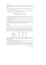
to consider Feynman diagrams which physicists use currently in the computations of
quantum field theory. Let us contemplate the diagram:
y
x
Figure 2
which is involved in the computation of the self-energy of an electron in QED. The
two points x and y of space-time at which the photon (the wiggly line) is emitted and
reabsorbed are very close by and our ansatz for ds will be at the intuitive level,
ds = ×−−−× . (56)
The right hand side has good meaning in physics, it is called the Fermion propagator
16

and is given by
where D is the Dirac operator.
We thus arrive at the following basic ansatz,
×−−−× = D −1 (57)
ds = D −1 . (58)
In some sense it is simpler than the ansatz giving ds 2 as g µν dx µ dx ν , the point being
that the spin structure allows really to extract the square root of ds 2 (as is well known
Dirac found the corresponding operator as a differential square root of a Laplacian).
The first thing we need to do is to check that we are still able to measure distances
with our “unit of length” ds. In fact we saw in the discussion of the quantized calculus
that variables with continuous range cant commute with “infinitesimals” such as ds
and it is thus not very surprising that this lack of commutativity allows to compute, in
the classical Riemannian case, the geodesic distance d(x, y) between two points. The
precise formula is
d(x, y) = Sup {|f(x) − f(y)| ; f ∈ A , ‖[D, f]‖ ≤ 1} (59)
where D = ds −1 as above and A is the algebra of smooth functions. Note that ds has
the dimension of a length L, D has dimension L −1 and the above expression for d(x, y)
also has the dimension of a length.
Thus we see in the classical geometric case that both the fundamental cycle in K-
homology and the metric are encoded in the spectral triple (A, H, D) where A is the
algebra of functions acting in the Hilbert space H of spinors, while D is the Dirac
operator.
To get familiar with this notion one should check that one recovers the volume form of
the Riemannian metric by the equality (valid up to a normalization constant [12])
∫ ∫
−f |ds| n = f √ g d n x (60)
M n
but the first interesting point is that besides this coherence with the usual computations
there are new simple questions we can ask now such as ”what is the two-dimensional
measure of a four manifold” in other words ”what is its area ” Thus one should
compute
∫
− ds 2 (61)
It is obvious from invariant theory that this should be proportional to the Hilbert–
Einstein action, the direct computation was done by D. Kastler and gives,
∫
− ds 2 = −1 ∫
r √ g d 4 x (62)
48π 2 M 4
where as above dv = √ g d 4 x is the volume form, ds = D −1 the length element, i.e. the
inverse of the Dirac operator and r is the scalar curvature.
In the general framework of Noncommutative Geometry the confluence of the Hilbert
space incarnation of the two notions of metric and fundamental class for a manifold
lead very naturally to define a geometric space as given by a spectral triple:
(A, H, D) (63)
17

where A is a concrete algebra of coordinates represented on a Hilbert space H and the
operator D is the inverse of the line element.
ds = 1/D. (64)
This definition is entirely spectral; the elements of the algebra are operators, the points,
if they exist, come from the joint spectrum of operators and the line element is an
operator.
The basic properties of such spectral triples are easy to formulate and do not make any
reference to the commutativity of the algebra A. They are
[D, a] is bounded for any a ∈ A , (65)
D = D ∗ and (D + λ) −1 is a compact operator ∀ λ ∉ C . (66)
(Of course D is an unbounded operator).
There is no difficulty to adapt the above formula for the distance in the general noncommutative
case, one uses the same, the points x and y being replaced by arbitrary
states ϕ and ψ on the algebra A. Recall that a state is a normalized positive linear
form on A such that ϕ(1) = 1,
ϕ : Ā → C , ϕ(a ∗ a) ≥ 0 , ∀ a ∈ Ā , ϕ(1) = 1 . (67)
The distance between two states is given by,
d(ϕ, ψ) = Sup {|ϕ(a) − ψ(a)| ; a ∈ A , ‖[D, a]‖ ≤ 1} . (68)
The significance of D is two-fold. On the one hand it defines the metric by the above
equation, on the other hand its homotopy class represents the K-homology fundamental
class of the space under consideration.
There is an equally simple formula for the Yang-Mills action in general The analogue of
the Yang-Mills action functional and the classification of Yang-Mills connections on the
noncommutative tori were developped in [20], with the primary goal of finding a ”manifold
shadow” for these noncommutative spaces. These moduli spaces turned out indeed
to fit this purpose perfectly, allowing for instance to find the usual Riemannian space of
gauge equivalence classes of Yang-Mills connections as an invariant of the noncommutative
metric. We refer to [12] for the construction of the metrics on noncommutative tori
from the conceptual point of view. All natural axioms of noncommutative geometry
are fulfilled in that case.
These constructions were greatly generalised to isospectral deformations of Riemannian
geometries of rank > 1 in joint work with G. Landi and M. Dubois-Violette .
In essence the transition from the Riemannian paradigm of geometry to the above spectral
one parallels the evolution of the unit of length in physics. The ”meter” for instance
was defined in the eighteen century as a small fraction of the earth circonference, and
concretely represented by a platinum bar localized near Paris. The actual standard of
length is given nowadays in a quite different way: it is the wave-length corresponding to
specific transitions in the cesium atom. The inverse frequencies are computed from the
corresponding Dirac Hamiltonian in exact analogy with the above spectral definition
of ”ds”. This unit of length is no longer localized, owing to its lack of commutativity
with the space-time coordinates.
18

There is a very important test of our general framework of geometry which is its compatibility
with what we know of space-time. The best way is to start with the hard
core information one has from physics and that can be summarized by a Lagrangian.
This Lagrangian is the Einstein Lagrangian plus the minimally coupled standard model
Lagrangian. How do we recover this action functional which contains both the Einstein-
Hilbert term as well as the standard model The answer is very simple: the Fermionic
part of this action is used to determine a spectral triple (A, H, D), where the algebra
A encodes not only the ordinary space-time (coming from QED) but also the internal
symmetries, the Hilbert space H encodes not only the ordinary spinors (coming from
QED) but all quarks and leptons, and the operator D encodes not only the ordinary
Dirac operator but also the Yukawa coupling matrix. Then one recovers the bosonic
part as follows. Both the Hilbert–Einstein action functional for the Riemannian metric,
the Yang–Mills action for the vector potentials, the self interaction and the minimal
coupling for the Higgs fields all appear with the correct signs in the asymptotic expansion
for large Λ of the number N(Λ) of eigenvalues of D which are ≤ Λ (cf. [4]),
N(Λ) = # eigenvalues of D in [−Λ, Λ]. (69)
This step function N(Λ) is the superposition of two terms,
N(Λ) = 〈N(Λ)〉 + N osc (Λ).
The oscillatory part N osc (Λ) is the same as for a random matrix, governed by the
statistic dictated by the symmetries of the system and does not concern us here. The
average part 〈N(Λ)〉 is computed by a semiclassical approximation from local expressions
involving the familiar heat equation expansion and delivers the correct terms.
Other nonzero terms in the asymptotic expansion are cosmological, Weyl gravity and
topological terms. We showed with G. Landi and M. Dubois-Violette that if one studies
natural presentations of the algebra generated by A and D one naturally gets only metrics
with a fixed volume form so that the bothering cosmological term does not enter
in the variational equations associated to the spectral action 〈N(Λ)〉. It is tempting
to speculate that the phenomenological Lagrangian of physics, combining matter and
gravity appears from the solution of an extremely simple operator theoretic equation.
In the spectral noncommutative framework the notion of curvature comes from the
local computation of the analogue of Pontrjagin classes: i.e. of the components of the
cyclic cocycle which is the Chern character of the K-homology class of D and which
make sense in general. This result allows, using the infinitesimal calculus, to go from
local to global in the general framework of spectral triples (A, H, D).
The Fredholm index of the operator D determines (we only look at the odd case for
ϕ
simplicity but there are similar formulas in the even case) an additive map K 1 (A) → Z
given by the equality
ϕ([u]) = Index (P uP ) , u ∈ GL 1 (A) (70)
where P is the projector P = 1+F , F = Sign (D).
2
It is an easy fact that this map is computed by the pairing of K 1 (A) with the following
cyclic cocycle
τ(a 0 , . . . , a n ) = Trace (a 0 [F, a 1 ] . . . [F, a n ]) ∀ a j ∈ A (71)
19

where F = Sign D and we assume that the dimension p of our space is finite, which
means that (D + i) −1 is of order 1/p, also n ≥ p is an odd integer. There are similar
formulas involving the grading γ in the even case, and it is quite satisfactory that both
cyclic cohomology and the chern Character formula adapt to the infinite dimensional
case in which the only hypothesis is that exp(−D 2 ) is a trace class operator.
The cocycle τ is however nonlocal in general because the formula (71) involves the
ordinary trace instead of the local trace ∫ − and it is crucial to obtain a local form of
the above cocycle.
This problem is solved in our joint work with Henri Moscovici ([18]). We make the
following regularity hypothesis on (A, H, D)
a and [D, a] ∈ ∩ Dom δ k , ∀ a ∈ A (72)
where δ is the derivation δ(T ) = [|D|, T ] for any operator T .
We let B denote the algebra generated by δ k (a), δ k ([D, a]). The usual notion of dimension
of a space is replaced by the dimension spectrum which is the subset of
{z ∈ C, Re(z) ≥ 0} of singularities of the analytic functions
ζ b (z) = Trace (b|D| −z ) Re z > p , b ∈ B . (73)
The dimension spectrum of an ordinary manifold M is the set {0, 1, . . . , n}, n = dim M;
it is simple. Multiplicities appear for singular manifolds. Cantor sets provide examples
of complex points z /∈ R in the dimension spectrum.
We assume that Σ is discrete and simple. Let (A, H, D) be a spectral triple satisfying
the hypothesis (72) and (73). The local index theorem is the following, [18]:
1. The equality ∫
−P = Res z=0 Trace (P |D| −z )
defines a trace on the algebra generated by A, [D, A] and |D| z , where z ∈ C.
2. There is only a finite number of non–zero terms in the following formula which
defines the odd components (ϕ n ) n=1,3,... of a cocycle in the bicomplex (b, B) of A,
ϕ n (a 0 , . . . , a n ) = ∑ k
c n,k
∫−a 0 [D, a 1 ] (k 1) . . . [D, a n ] (kn) |D| −n−2|k| ∀ a j ∈ A
where the following notations are used: T (k) = ∇ k (T ) and ∇(T ) = D 2 T − T D 2 ,
k is a multi-index, |k| = k 1 + . . . + k n ,
c n,k = (−1) √ (
|k| 2i(k 1 ! . . . k n !) −1 ((k 1 +1) . . . (k 1 +k 2 +. . .+k n +n)) −1 Γ |k| + n )
.
2
3. The pairing of the cyclic cohomology class (ϕ n ) ∈ HC ∗ (A) with K 1 (A) gives the
Fredholm index of D with coefficients in K 1 (A).
The first test of this general local index formula was the computation of the local
Pontrjagin classes in the case of foliations. Their transverse geometry is, as explained
20

in [18], encoded by a spectral triple. The answer for the general case [19], was obtained
thanks to a Hopf algebra H(n) only depending on the codimension n of the foliation. It
allowed to organize the computation and to encode algebraically the noncommutative
curvature. It also dictated the correct generalization of cyclic cohomology for Hopf
algebras. Another case of great interest came recently from quantum groups where
the local index formula works fine and yields quite remarkable formulas even in the
simplest case of SU q (2).
At about the same time as the Hopf algebra H(n), another Hopf algebra was discovered
by Dirk Kreimer, as the organizing concept in the computations of renormalization in
quantum field theory.
His Hopf algebra is commutative as an algebra and we showed that it is the dual Hopf
algebra of the envelopping algebra of a Lie algebra G whose basis is labelled by the one
particle irreducible Feynman graphs. The Lie bracket of two such graphs is computed
from insertions of one graph in the other and vice versa. The corresponding Lie group
G is the group of characters of H.
We showed that the group G is a semi-direct product of an easily understood abelian
group by a highly non-trivial group closely tied up with groups of diffeomorphisms.
Our joint work shows that the essence of the concrete computations performed by
physicists in the renormalization technique is conceptually understood as a special
case of a general principle of multiplicative extraction of finite values coming from the
Riemann-Hilbert problem. The Birkhoff decomposition is the factorization
γ (z) = γ − (z) −1 γ + (z) z ∈ C (74)
where we let C ⊂ P 1 (C) be a smooth simple curve, C − the component of the complement
of C containing ∞ ∉ C and C + the other component. Both γ and γ ± are loops
with values in G,
γ (z) ∈ G ∀ z ∈ C
and γ ± are boundary values of holomorphic maps (still denoted by the same symbol)
γ ± : C ± → G . (75)
The normalization condition γ − (∞) = 1 ensures that, if it exists, the Birkhoff decomposition
is unique (under suitable regularity conditions).
When G is a simply connected nilpotent complex Lie group the existence (and uniqueness)
of the Birkhoff decomposition is valid for any γ. When the loop γ : C → G
extends to a holomorphic loop: C + → G, the Birkhoff decomposition is given by
γ + = γ, γ − = 1. In general, for z ∈ C + the evaluation,
γ → γ + (z) ∈ G (76)
is a natural principle to extract a finite value from the singular expression γ(z). This
extraction of finite values coincides with the removal of the pole part when G is the
additive group C of complex numbers and the loop γ is meromorphic inside C + with z
as its only singularity.
The main result of our joint work ([16]) is that the renormalized theory is just the
evaluation at z = D of the holomorphic part γ + of the Birkhoff decomposition of the
loop γ with values in G provided by the dimensional regularization.
21

In fact the relation that we uncovered in [16] between the Hopf algebra of Feynman
graphs and the Hopf algebra of coordinates on the group of formal diffeomorphisms of
the dimensionless coupling constants of the theory allows to prove the following result
which for simplicity deals with the case of a single dimensionless coupling constant.
Let the unrenormalized effective coupling constant g eff (ε) be viewed as a formal power
series in g and let g eff (ε) = g eff+ (ε) (g eff− (ε)) −1 be its (opposite) Birkhoff decomposition
in the group of formal diffeomorphisms. Then the loop g eff− (ε) is the bare coupling
constant and g eff+ (0) is the renormalized effective coupling.
This allows, using the relation between the Birkhoff decomposition and the classification
of holomorphic bundles, to encode geometrically the operation of renormalization. It
also signals a very clear analogy between the renormalization group as an ”ambiguity”
group of physical theories and the missing Galois theory at Archimedian places alluded
to above. We refer to [14] for a detailed account of this analogy.
I
References
[1] M.F. Atiyah, Global theory of elliptic operators, Proc. Internat. Conf. on
Functional Analysis and Related Topics (Tokyo, 1969) University of Tokyo
press, Tokyo, (1970), 21-30.
[2] P. Baum and A. Connes, Geometric K-theory for Lie groups and foliations.
Preprint IHES (M/82/), 1982, to appear in l’Enseignement Mathematique,
t.46 (2000), 1-35.
[3] L.G. Brown, R.G. Douglas and P.A. Fillmore, Extensions of C ∗ -algebras and
K-homology, Ann. of Math. 2, 105 (1977), 265-324.
[4] A. Chamseddine and A. Connes: Universal formulas for noncommutative geometry
actions, Phys. Rev. Letters 77 24 (1996), 4868-4871.
[5] J. Chabert, S. Echterhoff, R. Nest, The Connes-Kasparov conjecture for almost
connected groups, MathQA/0110130.
[6] A. Connes, Une classification des facteurs de type III, Ann. Sci. Ecole Norm.
Sup., 6, n. 4 (1973), 133-252.
[7] A. Connes, Classification of injective factors, Ann. of Math., 104, n. 2 (1976),
73-115.
[8] Connes, A., C ∗ algèbres et géométrie differentielle. C.R. Acad. Sci. Paris,
Ser. A-B 290 (1980).
[9] A. Connes, Noncommutative differential geometry. Part I: The Chern character
in K-homology, Preprint IHES (M/82/53), 1982; Part II: de Rham homology
and noncommutative algebra, Preprint IHES (M/83/19), 1983. Noncommutative
differential geometry, Inst. Hautes Etudes Sci. Publ. Math. 62
(1985), 257-360.
[10] Connes, A., : Cohomologie cyclique et foncteur Ext n . C.R. Acad. Sci. Paris,
Ser.I Math 296 (1983).
22

[11] A. Connes: Cyclic cohomology and the transverse fundamental class of a
foliation, Geometric methods in operator algebras, (Kyoto, 1983), pp. 52-144,
Pitman Res. Notes in Math. 123 Longman, Harlow (1986).
[12] A. Connes: Noncommutative geometry, Academic Press (1994).
[13] A. Connes, Noncommutative Geometry and the Riemann Zeta Function, invited
lecture in IMU 2000 volume, to appear.
[14] A. Connes, Symétries Galoisiennes et renormalisation. Séminaire H. Poincaré
(2002).
[15] A. Connes, M. Douglas, A. Schwarz, Noncommutative geometry and Matrix
theory: compactification on tori, J. High Energy Physics, 2 (1998).
[16] A. Connes, D. Kreimer, Renormalization in quantum field theory and the
Riemann-Hilbert problem I: the Hopf algebra structure of graphs and the
main theorem. hep-th/9912092. Renormalization in quantum field theory and
the Riemann-Hilbert problem II: The β function, diffeomorphisms and the
renormalization group. hep-th/0003188.
[17] A. Connes and H. Moscovici: Cyclic cohomology, the Novikov conjecture and
hyperbolic groups, Topology 29 (1990), 345-388.
[18] A. Connes and H. Moscovici: The local index formula in noncommutative
geometry, GAFA, 5 (1995), 174-243.
[19] Connes, A. and Moscovici, H., Hopf Algebras, Cyclic Cohomology and the
Transverse Index Theorem, Commun. Math. Phys. 198, (1998) 199-246.
[20] A. Connes and M. Rieffel, Yang-Mills for noncommutative two tori, Operator
algebras and mathematical physics, (Iowa City, Iowa, 1985), pp. 237-266; Contemp.
Math. Oper. Algebra Math. Phys. 62, Amer. Math. Soc., Providence,
RI, 1987.
[21] A. Connes and M. Takesaki, The flow of weights on factors of type III, Tohoku
Math. J., 29 (1977), 473-575.
[22] U. Haagerup, Connes’ bicentralizer problem and uniqueness of the injective
factor of type III 1 , Acta Math., 158 (1987), 95-148.
[23] D. Kastler, The Dirac operator and gravitation, Commun. Math. Phys. 166
(1995), 633-643.
[24] D. Kastler, Noncommutative geometry and fundamental physical interactions:
The lagrangian level, Journal. Math. Phys. 41 (2000), 3867-3891.
[25] G.G. Kasparov, The operator K-functor and extensions of C ∗ algebras, Izv.
Akad. Nauk SSSR, Ser. Mat. 44 (1980), 571-636; Math. USSR Izv. 16 (1981),
513-572.
[26] W. Krieger, On ergodic flows and the isomorphism of factors, Math. Ann.,
223 (1976), 19-70.
23

[27] M. Pimsner, and D. Voiculescu, Exact sequences for K groups and Ext group
of certain crossed product C ∗ -algebras. J. Operator Theory 4 (1980), 93-118.
[28] M.A. Rieffel: Morita equivalence for C ∗ -algebras and W ∗ -algebras, J. Pure
Appl. Algebra 5 (1974), 51-96.
[29] M.A. Rieffel: The cancellation theorem for projective modules over irrational
rotation C ∗ -algebras, Proc. London Math. Soc. 47 (1983), 285-302.
[30] G. Skandalis: Approche de la conjecture de Novikov par la cohomologie cyclique.
Seminaire Bourbaki, (1990-91), Expose 739, 201-202-203 (1992),
299-316. P. Julg : Travaux de N. Higson et G. Kasparov sur la conjecture
de Baum-Connes. Seminaire Bourbaki, (1997-98), Expose 841, 252 (1998),
151-183.
G. Skandalis: Progres recents sur la conjecture de Baum-Connes, contribution
de Vincent Lafforgue. Seminaire Bourbaki, (1999-2000), Expose 869.
[31] M. Takesaki, Tomita’s theory of modular Hilbert algebras and its applications,
Lecture Notes in Math. 128, Springer (1970).
[32] B.L. Tsygan, Homology of matrix Lie algebras over rings and the Hochschild
homology, Uspekhi Math. Nauk. 38 (1983), 217-218.
[33] M. Wodzicki: Noncommutative residue, Part I. Fundamentals K-theory, arithmetic
and geometry, Lecture Notes in Math., 1289, Springer-Berlin (1987).
24