Pseudo-spectral derivative of quadratic quasi-interpolant splines

360 S. Remogna
1
3
0.9
0.8
2
0.7
1
0.6
0.5
0
0.4
0.3
−1
0.2
−2
0.1
0
−3 −2 −1 0 1 2 3
(a)
−3
−3 −2 −1 0 1 2 3
(b)
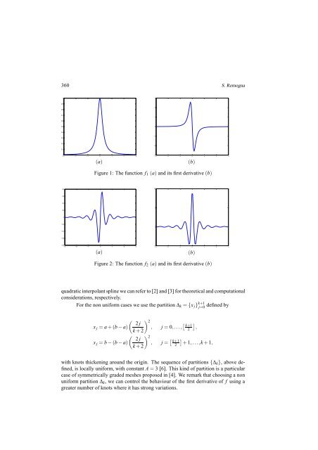
Figure 1: The function f 1 (a) and its first derivative(b)
0.8
10
0.6
0.4
0.2
5
0
−0.2
0
−0.4
−0.6
−0.8
−3 −2 −1 0 1 2 3
(a)
−5
−3 −2 −1 0 1 2 3
(b)
Figure 2: The function f 2 (a) and its first derivative(b)
quadratic interpolant spline we can refer to [2] and [3] for theoretical and computational
considerations, respectively.
For the non uniform cases we use the partition ∆ k ={x j } k+1
j=0
defined by
( 2 j
x j = a+(b−a)
k+2
x j = b−(b−a)
( 2 j
k+2
) 2
, j = 0,..., [ ]
k+1
2 ,
) 2
, j = [ ]
k+1
2 + 1,...,k+1,
with knots thickening around the origin. The sequence of partitions {∆ k }, above defined,
is locally uniform, with constant A=3 [6]. This kind of partition is a particular
case of symmetrically graded meshes proposed in [4]. We remark that choosing a non
uniform partition ∆ k , we can control the behaviour of the first derivative of f using a
greater number of knots where it has strong variations.